Finite Element Analysis of Hybrid Boron-carbon Composites

FINITE ELEMENT ANALYSIS OF HYBRID BORON-CARBON COMPOSITES

ABSTRACT

Adaptability to different situations and the ease of combination makes composites one of the most extensively used materials in the engineering industries. One of the ways of managing properties of composites is hybridization of different fibers in one composite.

This work merely focuses upon the analysis of effective stiffness of Hybrid materials which is carried out using Finite Element Method.

A series of models were experimented in a sequence by imposing various conditions on each of them. Boron and Carbon fibers were used primarily for these experiments because of their better compatibility than other combinations of fibers.  Due to the difference in diameters of the fibers it was possible to achieve very high volume concentration of fibers. Longitudinal properties of hybrid composites are studied well in literature but prediction of transversal properties was a challenge. The results of FEM modelling were compared with the theoretical predictions and conclusions were drawn.

TABLE OF CONTENTS

ACKNOWLEDGEMENTS………………………………………………………..

ABSTRACT……………………………………………………………………….

LIST OF ILLUSTRATIONS……………………………………………………………….

LIST OF TABLES…………………………………………………………………

Chapter 1 INTRODUCTION………………………………………………………

1. Composites: Definition and Classification………………………………
2. Classification of Composite Materials…………………………………..
3. Previous Studies on Hybrid Composites………………………………..
4. Objectives of Present Study…………………………………………….

Chapter 2 LITERATURE REVIEW………………………………………………..

Chapter 3 MATERIAL SPECIFICATION…………………………………………

Chapter 4 FE MODELING AND SIMULATION…………………………………

4.1 Modeling Steps……………………………………………………………

4.2 Cases Studied……………………………………………………………..

4.2.1 Triangular Models…………………………………………………….

4.2.2 Hexagonal Models……………………………………………………

4.2.3 Rectangular Models…………………………………………………..

Chapter 5 RESULTS AND DISCUSSION

5.1 Results of Triangular Models…………………………………………..

5.1.1 Estimation of Longitudinal Properties………………………………

5.1.2 Behavior of Elastic Strain on Infinite Lengths…………………………….

5.1.3 Estimation of Transversal Properties………………………………..

5.2 Results of Rectangular Models……………………………………………….

5.2.1 Estimation of Longitudinal Shear Stiffness………………………….

5.2.2 Estimation of Transversal Shear Stiffness…………………………..

Chapter 6 CONCLUSION……………………………………………………………….

6.1 Summary and Conclusion…………………………………………………….

6.2 Future Work……………………………………………………………………

REFERENCES…………………………………………………………………………….

BIOGRAPHICAL INFORMATION………………………………………………………

LIST OF ILLUSTRATIONS

Figure 1.1 In-Layer and In-Ply hybridization………………………………………

Figure 4.1 Steps in modeling……………………………………………………….

Figure 4.2 Orthogonal and front view of Model 1………………………………….

Figure 4.3 Orthogonal and front view of Model 2………………………………….

Figure 4.4 Orthogonal and front view of Model 3………………………………….

Figure 4.5 Symmetry cut view of Triangular Model 1……………………………..

Figure 4.6 Front face meshing of Triangular Model 1…………………………….

Figure 4.7 Boundary conditions on Triangular Model 1…………………………..

Figure 4.8 Boundary conditions on Triangular Model 2…………………………..

Figure 4.9 Symmetry cut view of Triangular Model 3……………………………

Figure 5.0 Meshing on Triangular Model 3……………………………………….

Figure 4.11 Front view of Triangular Model 3……………………………………..

Figure 4.12 Fine meshing of carbons and matrix…………………………………..

Figure 4.13 Direct compressive pressure applied on Model 2 by increasing the  length to 4000µm………………………………………………………………….

Figure 4.14 Direct tensile pressure applied on a Model 2 by increasing the  length to 4000µm…………………………………………………………………………..

Figure 4.15 Hexagonal model 1……………………………………………………

Figure 4.16 Hexagonal model 2…………………………………………………

Figure 4.17 Hexagonal model 3…………………………………………………….

Figure 4.18 Meshing of Rectangular Model……………………………………….

Figure 4.19 Boundary Conditions on Rectangular model 1 in longitudinal directions…………………………………………………………………………..

Figure 4.20 Boundary Conditions on Rectangular model 1 in transversal directions……………………………………………………………………………

Figure 5.1 Distribution of Normal Stresses on Triangular Model 1……………….

Figure 5.2 Distributtion of Normal stresses on all the three Triangular Models……

Figure 5.3 Distribution of Normal Elastic Strains on Triangular Model 1 in Transversal and Longitudinal directions…………………………………………..

Table 5.4 Comparison of Theoretical and FE Model values of Shear Modulus in Longitudinal and Transversal Direction for Rectangular Model 1 and 2…………..

Figure 5.5 Plot between Total Concentration of Fibers and Poisson’s Ratio in Longitudinal Direction……………………………………………………………

Figure 5.6 Plot between Total Concentration of Fibers and Young’s Modulus in Transversal Direction…………………………………………………………….

Figure 5.7 Plot between Total Concentration of Fibers and Poisson’s Ratio in Transversal Direction…………………………………………………………….

Figure 5.8 Normal Elastic Strain of Triangular Model 1 in Axial Direction…….

Figure 5.9 Normal Elastic Strain of Triangular Model 1 increased to length 4000µm in Axial Direction…………………………………………………..

Figure 5.10 Deformation of Rectangular Model 1 subjected to Longitudinal Shear force………………………………………………………………………….

Figure 5.11 Surface Displacements of Rectangular Model 1 subjected to Longitudinal Shear force…………………………………………………….

Figure 5.12 Deformation of Rectangular Model 1 subjected to Transversal Shear force…………………………………………………………………………….

Figure 5.13 Surface Displacements of Rectangular Model 1 subjected to Transversal Shear force…………………………………………………………

Figure 5.14 Plot between Total Concentration of Fibers and Shear Modulus in Longitudinal Direction………………………………………………………….

Figure 5.15 Plot between Total Concentration of Fibers and Shear Modulus in Transversal Direction……………………………………………………………

LIST OF TABLES

Table 3.1 Properties of Resin Epoxy Matrix……………………………………….

Table 3.2 Properties of Boron Fiber……………………………………………….

Table 3.3 Properties of Carbon (T300) Fiber………………………………………

Table 5.1 Table with Normal Stresses and Normal Strains based on the concentration of fibers and matrix for all the Triangular Models…………………

Table 5.2 Comparison of Theoretical and FE Model values of Young’s modulus and Poisson’s Ratio in axial direction for all the three Triangular Models…………

Table 5.3 Comparison of Theoretical and FE Model values of Young’s modulus and Poisson’s Ratio in Transversal Direction for all the three Triangular Models…

Table 5.4 Comparison of Theoretical and FE Model values of Shear Modulus in Longitudinal and Transversal Direction for Rectangular Model 1 and 2………….

Chapter 1

INTRODUCTION

1.1 Composites: Definition and Classification

Advanced composites are a blend of two or more distinct constituents or phases, of which one is made up of stiff, long fibers, and the other, a binder or matrix which holds the fibers in place. The composites thus formed are generally composed of layers or laminates of fibers and matrix. They have enhanced properties as compared to the constituents which retain their individual identities to influence the final properties. The fibers are tough and rigid relative to the matrix, with different properties in different directions, which means they are orthotropic. For the modern structural composites, the length to diameter ratio of fibers generally varies over 100.[1]

If well designed, a composite material usually exhibits the best qualities of its components or constituents. Composite materials are formed to get the best refined properties. Some of the properties that can be improved by forming a composite are strength, stiffness, corrosion resistance, wear resistance, attractiveness, weight, fatigue life, thermal insulation, thermal conductivity, and acoustic insulation. Not all these properties are upgraded at the same time but, depending on the task to be performed, characteristics are taken into consideration.[2]

Examples: The fibers and matrices are made out of various materials. The fibers are typically glass, carbon, silicon carbide, or asbestos, while the matrix is usually plastic, metal, or a ceramic material.

1.2 Classification of Composite Materials

Based on the type of reinforcements, the composite materials are primarily classified into two broad categories as Fiber Reinforced Composites and Particle Reinforced Composites.

In a Fiber Reinforced Composite, also known as a Fibrous Reinforcement, the length is much higher than its cross-sectional dimension. The ratio of length to cross-sectional dimension is known as aspect ratio. Single- layered fibers with high aspect ratio are called Continuous Fiber Reinforced Composites whereas, those with low aspect ratios are called Discontinuous Fiber Reinforced Composites. Depending on the orientation of the continuous fibers, the reinforcement can be either Unidirectional or Bidirectional. These bidirectional reinforcements can also be termed as Woven Reinforcements. Similarly, the discontinuous fibers may be Random oriented or Preferred oriented.

Multilayered Composites, being another group of the Fibrous Reinforcements, can be sub-grouped as, Laminates and Hybrids. By stacking layers or plies in a specific sequence, the Laminates are obtained. These are usually unidirectional. A typical laminate may have 4 to 40 layers, of which the fiber orientation changes from layer to layer. Multilayered composites with mixed fibers result in Hybrids, which are now becoming commonplace. These hybrid composites are designed to benefit from the properties of fibers employed. Here, the fibers can be mixed in a ply or layer by layer. Also, some hybrids have a mixture of fibrous and particulate reinforcements.

However, the particle reinforced composites have dimensions approximately equal in all directions. In this case, the shape of the particles are important which can be any regular or irregular geometry such as, spherical, cubic or platelet. Same as in Discontinuous Single-layered composites, the particulate reinforcements can also be arranged in a Random or Preferred manner.[3]

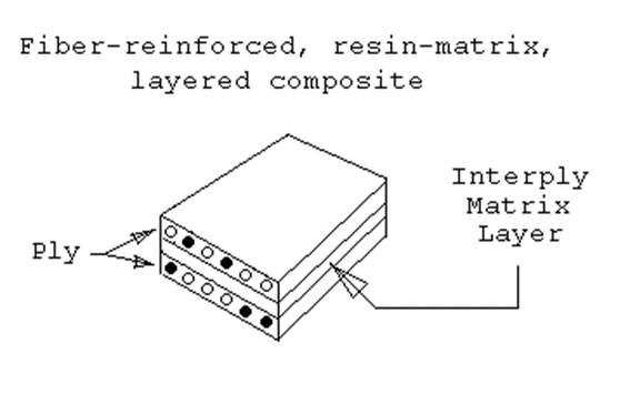
Figure 1.1 In-Layer and In-Ply hybridization

1.3 Previous Studies on Hybrid Composites

The term ‘Hybrid composite’ was coined in the fifties of the twentieth century and since then they have been studied and utilized till present. In the 1970s and 1980s, the theoretical analysis on hybrid composites was done. This was the time when most of the frequently used fibers like carbon, boron, Kevlar, and other fibers came into commercial existence. To analyze the materials for which the layers are made from different fibers, was a simple task but analyzing the case of in-ply hybridization, where different types of fibers are used to make unidirectionally reinforced materials, was intricate. Formerly, a number of experiments were conducted on in-ply hybrid composites for the estimation of  longitudinal and transversal properties. In all these approaches, the results of theoretical modeling of usual unidirectional composites were used. In this case, longitudinal stiffness of such material was estimated with sufficient precision using the ‘mixture rule’ and for the prediction of effective strength, the difference in ultimate strains is usually considered. Three types of models were considered for analysis, namely,

• Anisotropic Matrix Model
• Four-Phase Model
• Double Periodic Model

These models were being experimented for the longitudinal and transversal properties. Results obtained from these models were close enough to the theoretical results.

1.4 Objectives of Present Study

The principal objective of this work is to study the properties of hybrid composites and to determine the longitudinal and transversal characteristics by numerically computing the shear moduli. To accomplish this, a combination of fibers and matrix are examined by launching certain boundary conditions.

Here, boron and carbon are considered because they combine excellent mechanical properties as compared to the other fiber combinations. In the case of boron and carbon, the difference between the ultimate strains is relatively less due to which the chance of breaking is also less. Apart from this, their elastic properties are closer. Boron being highly resistive to compression, and carbon being highly resistive to tension,  together they exhibit better strength towards both compressive and tensile effects.

Experiments are done for shear moduli on various models with different volume concentrations of fibers, and effect of this is studied on all the models. This comprises of numerically computing the values, and comparing with the theoretical results.

Chapter 2

LITERATURE REVIEW

Hybridization is one of the effective and efficient ways of ameliorating the energy absorption capability of the fiber reinforced composite materials. Hybrid composite laminates reinforced with carbon, Kevlar, glass, natural fibers and other types of fibers have been studied over time.[6]

Earlier, Carbon fiber reinforced composites were utilized tremendously, because of their excellent mechanical properties making them popular for lightweight, high-performance applications. But because of their limitations such as low tensile failure strain and high-cost, hybrid composites came into existence. This was a method in which the drawbacks of one fiber can be balanced out by the virtues of the other.

Carbon and glass being the low and high elongation fibers respectively, is the most common combination of hybrid composites. Moreover, the properties of some hybrid composites go beyond the expected on the basic of consideration of rules-of-mixture, referred to as the hybrid effect. This was discovered by Hayashi in 1972. His findings deduced that the failure strain of an all-carbon fiber composite could be increased by 40% by introducing glass fibers. Finally, it was quoted that the three main causes for hybrid effect are residual thermal stresses, fracture propagation effects and dynamic stress concentrations.

The attempts of many authors to model hybrid composites were not always successful. They could analyze some of the influencing parameters but the conclusions were not straightforward and sufficient for them to interpret the results.[8] Later, a global load-sharing model was developed and study for carbon/glass fibers was carried out. This study gave out the directions for designing optimal hybrid composites [7].

Numerous investigations were done on hybrid laminates subjected to low velocity impact but very few dealt with ballistic impact on hybrid composites. One of which was the effect of hybridization with E-glass fabric on carbon/epoxy laminates [9]. Also, the influence of Kevlar 29 fibers on E-glass reinforced laminates was examined [10]. A work on basalt fibers reported to offer mechanical properties comparable with those of traditional glass ones while displaying advantages in terms of environmental sustainability and chemico-physical properties [11,12]. In addition to this, investigations were done by replacing glass fibers with basalt fibers to study the impact resistance, which proved to be successful. It was inferred that basalt fibers act as good impact resistance improvers for composite laminates with a view to enhance the environmental sustainability to such composites [7,13-15]. A further work on hybrid composites was done on the impact of high velocity behavior of hybrid basalt-carbon/epoxy composites. In this experiment, interply hybrid specimens with four stacking sequences were tested and compared to laminates made of either only carbon or basalt layers. The result was that the ballistic limits of all stacking sequences were enhanced when compared to those of either only carbon or basalt. Eventually, the response to impact in this case was largely improved. Also, since the basalt fibers are far less-expensive when compared to carbon, therefore the hybridization made it cost-effective [16].

Besides, there were also researches carried out on polymer matrix composites and metal/ceramic composites, which are generally used for the spacecraft applications. These were tested for hypervelocity impact behaviors since the spacecrafts have to overcome the force of the particles and meteoroids which move with high velocities in space. However, it was concluded that once the composites are affected by hypervelocity impact, spallations and delaminating as well as adiabatic shear tended to form [17,18]. In all these experiments, Ti was used as one of the fibers, since they can strengthen the anti-penetration ability for aluminum alloys. The combination of Ti and M40 was also tried on hypervelocity impact and the behavior of composites thin targets were observed. Results were positive as the composites presented high impact resistance [19].

Apart from spacecraft applications, hybrid composites in the form of tendons are widely used in civil infrastructures, buildings, and offshore infrastructure services as well. These are used as tension members and use high-tensile-strength steel wires, bars, and rebars which are ought to get corroded. To avoid this, the use of fiber-reinforced polymer matrix composites, especially carbon-fiber-reinforced polymer matrix composites was proposed [20,21]. Later, novel carbon/glass hybrid thermoplastic composite rods consisting of unidirectional PAN-based carbon fiber, braids of E-class glass fibers, and thermoplastic epoxy matrix was developed and checked for the tensile properties and fracture behavior. The tensile modulus and strength increased with the increasing carbon fiber volume fraction [22].

Chapter 3

MATERIAL SPECIFICATION

The primary requirement to carry out a simulation in Ansys is the characterization of materials and its properties. Since this analysis was on hybrid composites, two fibers and a matrix have been used who’s properties are highlighted below. To make a hybrid composite, the fibers and matrix must be selected in such a way that, it gives good properties in both longitudinal and transverse direction. In this study, Boron and Carbon were selected in combination with epoxy, due to better compatibility. Carbon being weaker in the transversal direction, becomes good when combined with boron, which exhibits better properties in both axial and transversal directions. The properties of these materials have been discussed below:

Resin Epoxy: Epoxies are polymerizable thermosetting resins and are available in a variety of viscosities from liquid to solid. Epoxies are used widely in resins for prepreg materials and structural adhesives. The advantages of epoxies are high strength and modulus, low levels of volatiles, excellent adhesion, low shrinkage, good chemical resistance, and ease of processing. Epoxy resins are often used as a matrix because they have excellent mechanical properties and good handling properties, including fabrication.

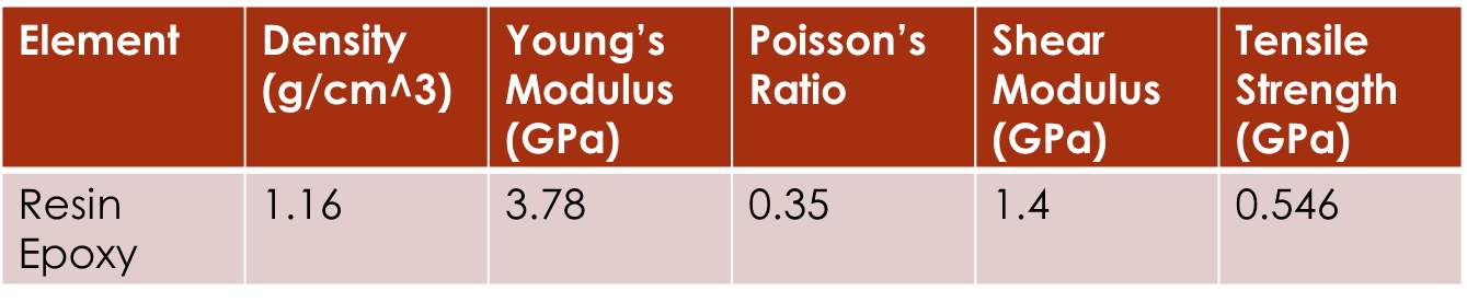
Table 3.1 Properties of Resin Epoxy Matrix

Boron: Boron fibers are very stiff and have a high tensile and compressive strength and possess excellent resistance to buckling. These fibers have relatively large diameters (usually 100-130µm) and do not flex well. They are usually considered for their light weight. Boron fibers are primarily used in military aviation applications, especially for the repair of cracks and patches.

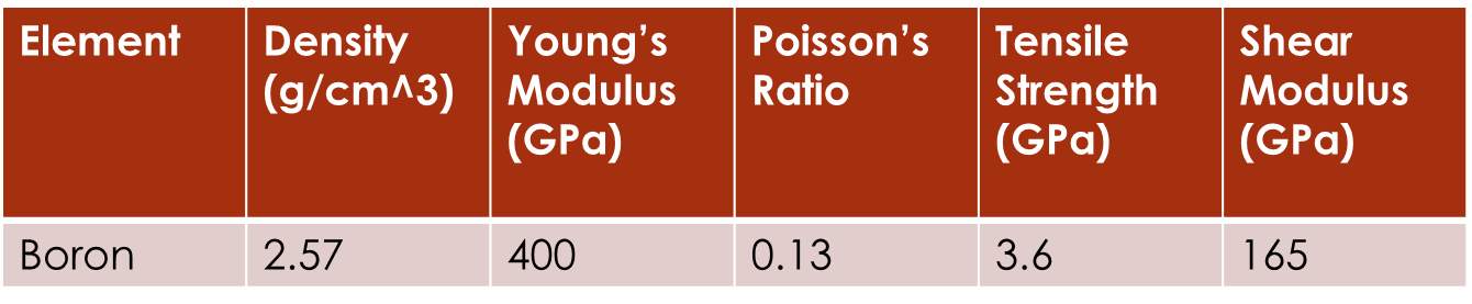
Table 3.2 Properties of Boron Fiber

Carbon: Carbon fibers are very stiff and strong, 3 to 10 times stiffer than glass fibers. Carbon fibers are used for structural aircraft applications. Advantages include, high strength and corrosion resistance.

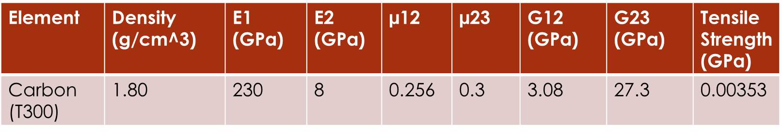
Table 3.3 Properties of Carbon (T300) Fiber

Chapter 4

FE MODELING AND SIMULATION

The finite element method (FEM) is a numerical method for solving problems of engineering and mathematical physics. Typical problem areas of interest include structural analysis, heat transfer, fluid flow, mass transport, and electromagnetic potential. The formulation of the problem  using finite element method results in a system of algebraic equations which yields approximate values of the unknowns at discrete number of points over the domain.[4] In this process, a model is subdivided into various small and simple geometries which become easy to solve. The subdivision of a whole domain into simpler parts has several advantages.[5]

• Accurate representation of complex geometry
• Inclusion of dissimilar material properties
• Easy representation of the total solution
• Capture of local effects.

4.1 Modeling Steps

In this research work the modelling was carried out using SolidWorks whereas the simulation was done in ANSYS (workbench). The process flowchart is as outlined below.

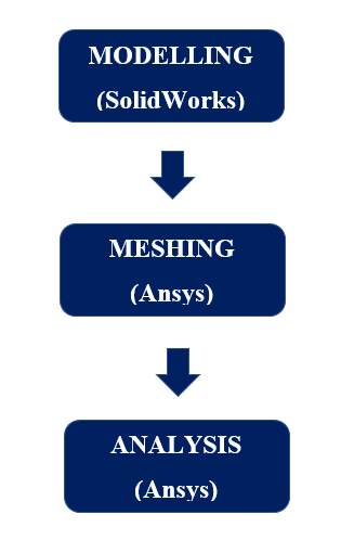
Figure 4.1 Steps in modeling

4.2 Cases Studied

A total of three models were experimented in this work each of them with varying volume concentrations of fibers and matrix. Boron and Carbon fibers were taken for hybridization and Resin Epoxy was taken as the matrix. Diameters of fibers were kept constant throughout the process, for boron fibers it was 100µm and for carbon it was 7.5µm and the length of the body was 2000µm.

In the first model, the volume of carbon fibers are relatively low when compared to the volume of boron fibers which in turn produces high buckling effect.

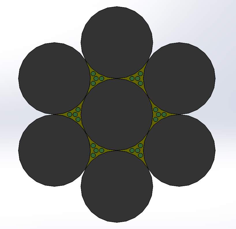
Figure 4.2 Orthogonal and front view of Model 1

The volumes concentrations of boron fibers and carbon fibers is approximately the same in the second model, which produces relatively low buckling effect as compared to the first model.

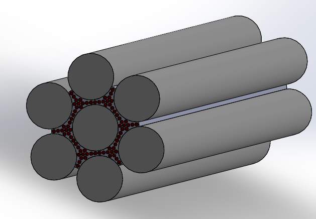
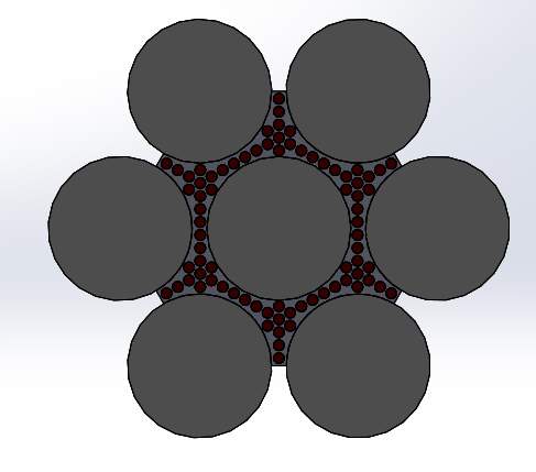
Figure 4.3 Orthogonal and front view of Model 2

In the final model, the effect of buckling becomes too low because of the high concentration of carbon fibers as shown in the figure below.

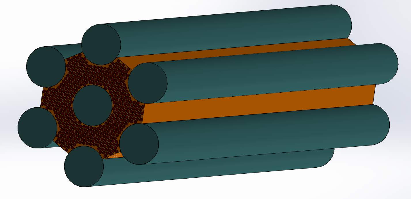
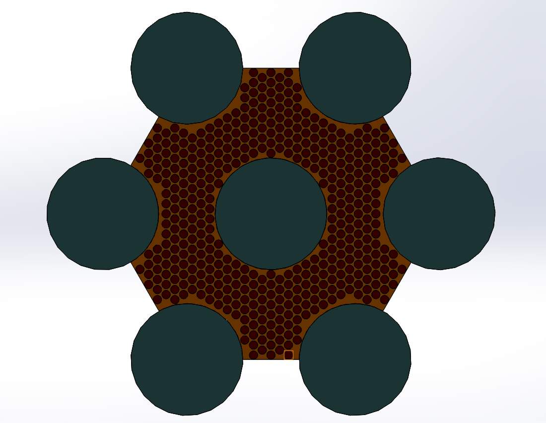
Figure 4.4 Orthogonal and front view of Model 3

4.2.1 Triangular Models

These models have been derived from the parent models which have been already illustrated in 3.2. For simplification, 1/6^th part of the models were cut using symmetry tool and analysis was performed on these models. For analysis, different pressures were applied in a way that it gets deformed in the longitudinal or axial direction and displacements were also applied to the bodies. Deformations and elastic strains were deduced.

Triangular Model 1:

In this case, the model was fixed on one surface and allowed to get displaced from the opposite surface by applying a pressure of 10MPA on the lateral surfaces. The model was then allowed to run on fine mesh which gave about 102706 nodes and 33277 elements in total.

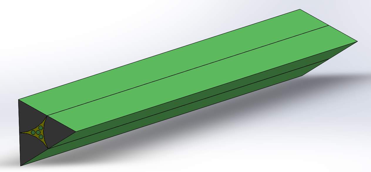
Figure 4.5 Symmetry cut view of Triangular Model 1

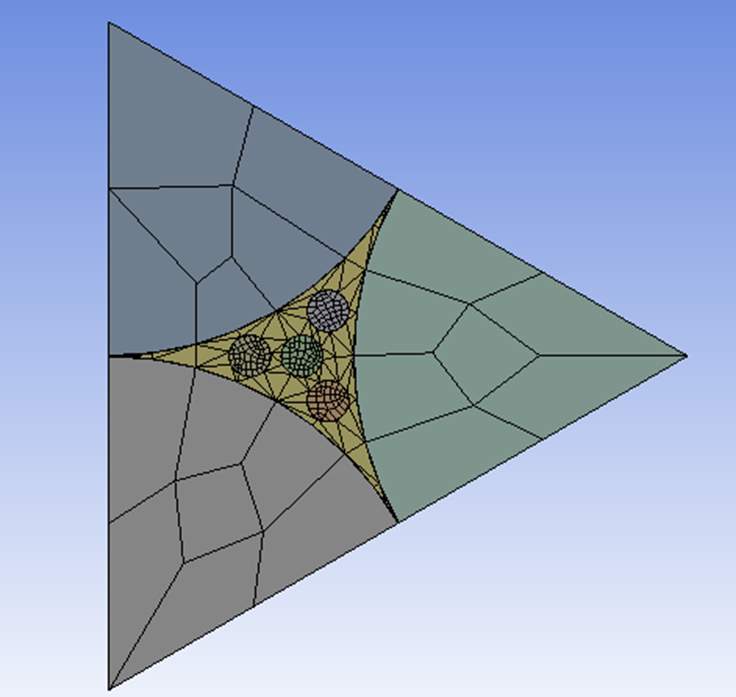
Figure 4.6 Front face meshing of Triangular Model 1

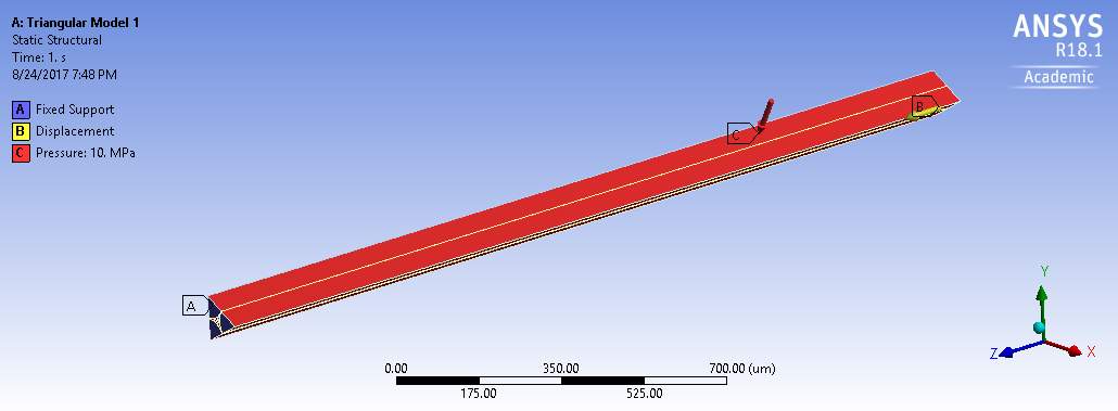
Figure 4.7 Boundary conditions on Triangular Model 1

Triangular Model 2:

With the same boundary conditions, the second model was also analyzed with an increase in the number of elements to 62652 which resulted in 308228 nodes. This increase was due to the increase in the number of carbon fibers.

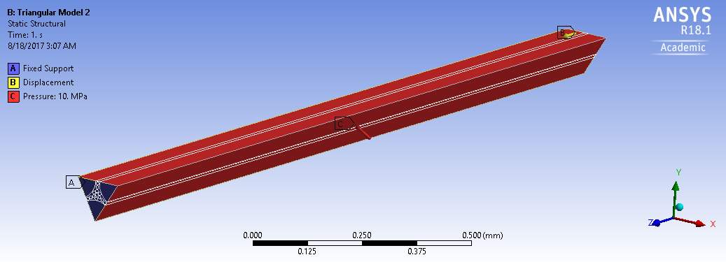
Figure 4.8 Boundary conditions on Triangular Model 2

Triangular Model 3:

Model 3 was experimented in the same way by applying similar boundary conditions but due to large number of parts it resulted in almost triple the number of nodes i.e.,866366 when compared to the second model and as much as 413704 elements.

All the above cases were used to analyze the Young’s modulus and Poisson’s ratio by numerical calculations using the normal stresses and strains which were inferred from the analysis.

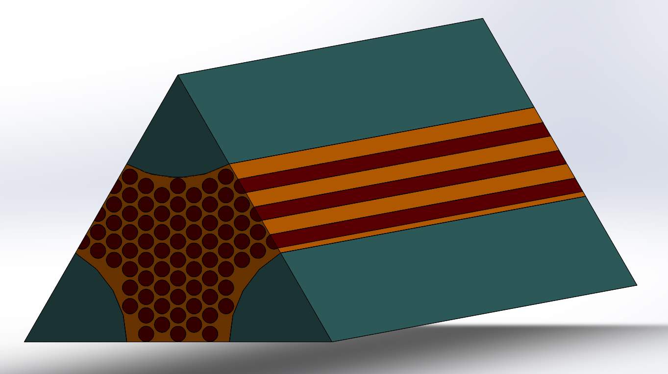
Figure 4.9 Symmetry cut view of Triangular Model 3

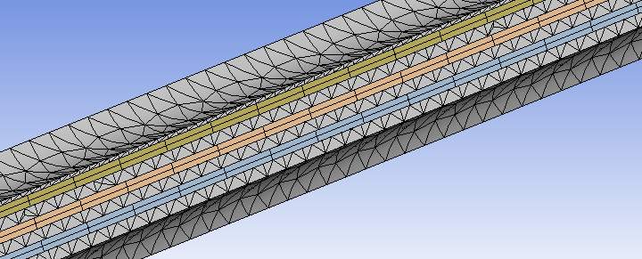
Figure 4.10 Meshing on Triangular Model 3

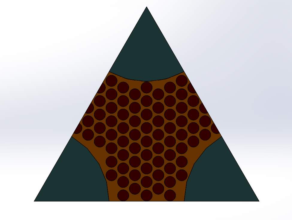
Figure 4.11 Front view of Triangular Model 3

Figure 4.12 Fine meshing of carbons and matrix

Furthermore, Triangular Model 2 was also experimented by increasing the length of the bar to 4000µm which was 2000µm previously. This was done to test the effect of strain the bar when the length goes on tending to infinity. Results were quite satisfactory. Below is the figure which shows the Triangular Model 2 but length 4000µm. The boundary conditions were the same as before.

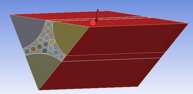
Figure 4.13 Direct compressive pressure applied on Model 2 by increasing the  length to 4000µm

Until now, the pressure was applied on the models in such a way that the deformation of body was in longitudinal direction, means the pressure applied was compressive. In addition to this, with similar boundary conditions, pressure was applied in such a manner that the body was subject to deformation in the direction perpendicular to the axis and results were compared. This was done to analyze the behavior of the bar on the application of tensile pressure. Just like the previous case, this comparison was also done on both 2000µm and 4000µm bar.

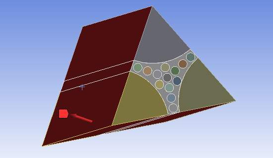
Figure 4.14 Direct tensile pressure applied on a Model 2 by increasing the length to 4000µm

In addition to this, the transversal properties were also estimated by taking the same models but with different boundary conditions. In the previous case, i.e., in the calculation of longitudinal properties, the body was allowed to deform in the axial direction whereas in this case, the body was allowed to move in the transversal direction and restricted in the axial direction. From this, the bulk modulus was computed and simultaneously the Young’s modulus and Poisson’s ratio were calculated.

4.2.2 Hexagonal Models

Same as the triangular models, the hexagonal models were also derived from the parent models. For this, two types of analysis were carried out on each of the three hexagonal models. In the first case, shear forces of varying magnitudes were applied on the lateral surfaces of the bodies in axial direction.

Hexagonal Model 1:

The first model constituted of 32 parts. As shown in the figure, the bottom surface was fixed and a pressure of 1MPA was applied on the top surface in such a way that it shears in the axial direction. On the remaining 4 sides a pressure of τcos60° was applied in opposite directions. Because of fewer parts, meshing was done fine.

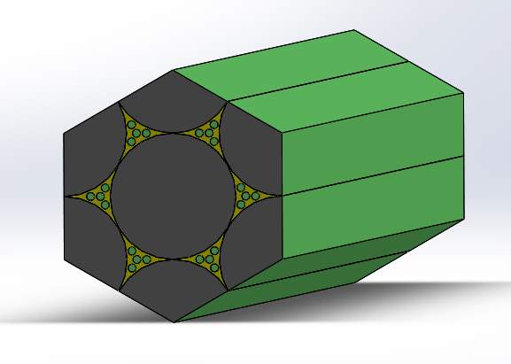
Figure 4.15 Hexagonal model 1

Hexagonal Model 2:

Likewise, model 2 was subjected to the above mentioned boundary conditions. With almost thrice the number of parts in the first model, it ran smooth on fine mesh.

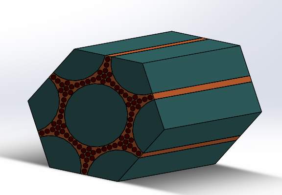
Figure 4.16 Hexagonal Model 2

Hexagonal Model 3:

This model consists of the highest number of parts amongst all the three models. Due to this huge number, it was very difficult to simplify using fine mesh. Therefore, medium mesh was considered in this regard. Besides this, all the other conditions imposed were the same.

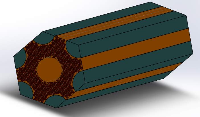
Figure 4.17 Hexagonal Model 3

Apart from the longitudinal shear force, another type of shear force was applied on the body as well which is called transverse shear force which acts exactly in the direction perpendicular to the axis. This operation was implemented on model 2, because of the same volume concentrations of both Boron and Carbon fibers.

In this analysis, again the bottom side is fixed and a force of 1MPA is applied on the top surface but in transverse direction, which allows shearing in transverse direction. Additionally, a shear force of τcos60° magnitude is applied on the rest of the lateral faces in opposite directions. Moreover, compressive and tensile forces were also allowed to act as detailed in the image below. The magnitude of these pressures were approximately τcos30°.

Due to the complexity in the calculation of shear forces to be applied on the lateral surfaces of the hexagonal body, meshing was done but simulations could not be carried out and therefore, these models were replaced by the rectangular models, which will be discussed in the next section.

4.2.3 Rectangular Models

A couple of experiments were conducted on a series of rectangular models and       the longitudinal and transversal shear moduli were determined. This was done to analyze the shear stiffness in both the directions. The meshing was done on these models as illustrated below. A superfine mesh was generated near the matrix and carbon fibers by the use of ‘body sizing’ with a size of about 2.5µm whereas, a regular mesh was generated for the boron fibers.

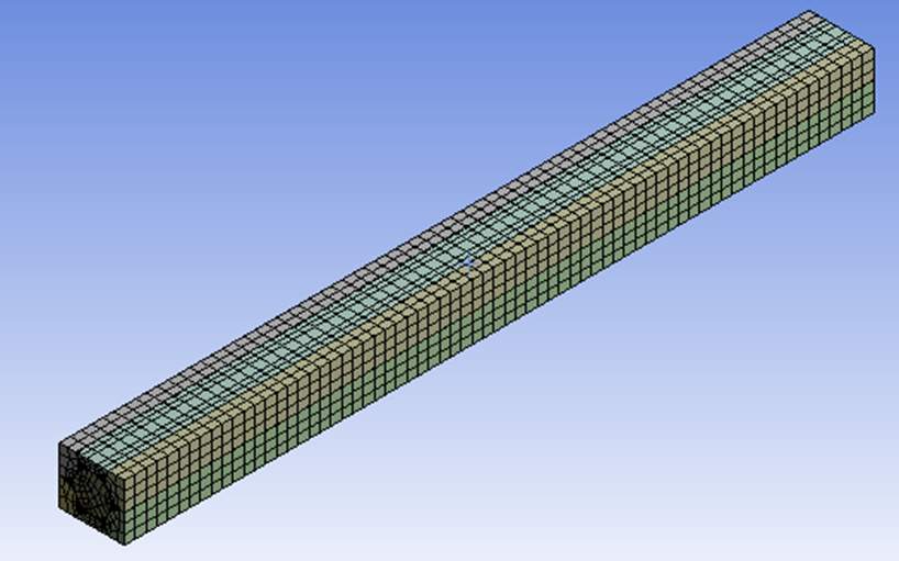
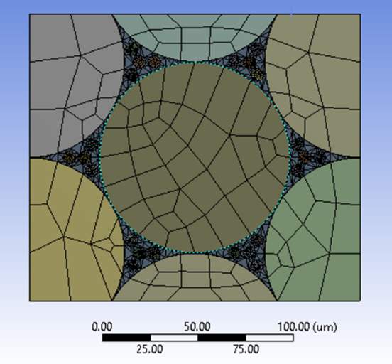
Figure 4.18 Meshing of Rectangular Model

Estimation of Longitudinal Shear Stiffness:

In the first experiment, the bottom surface was fixed and a pressure of 100MPa was applied on the top surface in axial direction. Due to this pressure, there is force created on the fixed support in the opposite direction which eventually creates a shear in the axial direction. This causes the body to get deformed and the surface displacements were then  determined using probe. With these displacements, the longitudinal shear modulus was calculated by various formulae.

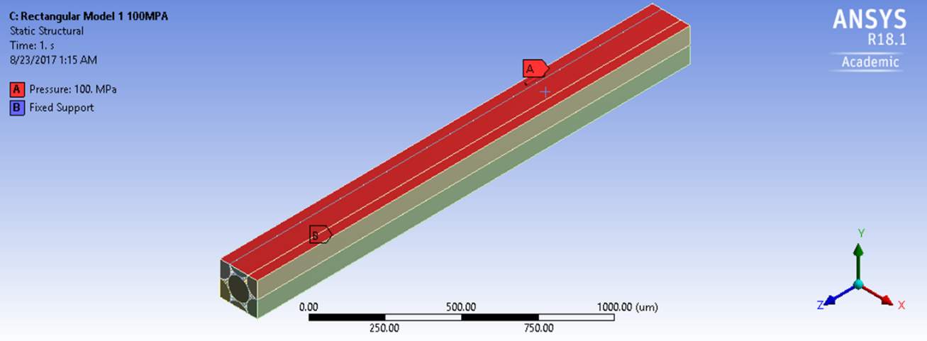
Figure 4.19 Boundary Conditions on Rectangular model 1 in longitudinal directions

Estimation of Transversal Shear Stiffness:

In the next experiment, the same boundary conditions were taken but the only difference was in the application of pressure. Here, the pressure was applied in the transversal direction due to which there was a shear force generated in the transversal direction and hence the displacements were recorded as done before. Using these displacements, the transversal shear modulus was deduced. In this case, due to the deformation, the body turns into a skewed shape. With this skewed angle, the shear angle and other properties were determined.

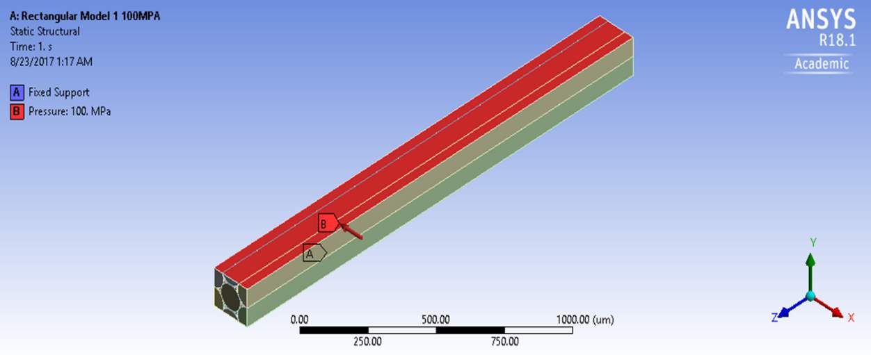
Figure 4.20 Boundary Conditions on Rectangular model 1 in longitudinal directions

In both longitudinal and transverse directions, analysis was carried out to obtain shear modulus for both Model 2 and Model 3. Considerable results were obtained for the second model, but, in the case of third model, because of limitation of number of nodes and elements, the model failed to run, as it containing 452 parts.

Chapter 5

RESULTS AND DISCUSSION

The results of all the models have been discussed in this chapter.

5.1 Results of Triangular Models

The first phase of simulations were done to determine the longitudinal and transversal properties.

5.1.1 Estimation of Longitudinal Properties

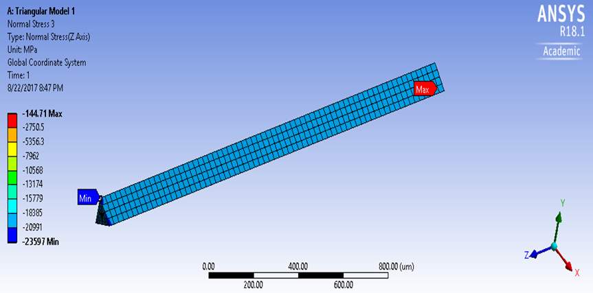
Figure 5.1 Distribution of Normal Stresses on Triangular Model 1

       

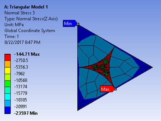
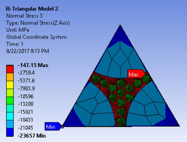
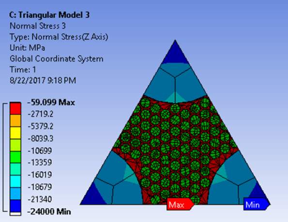
Figure 5.2 Distributtion of Normal stresses on all the three Triangular Models

The stresses induced in the body is proportional to the concentrations of fiber, was induced from the above analysis. As the volume of carbon and matrix keep increasing gradually, the model tends to become weak because of the low strength of carbon fibers and epoxy as compared to boron fibers.

The strains induced in all the directions are picturized below.

    

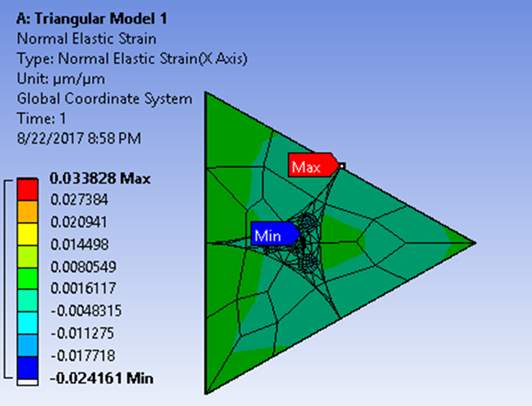
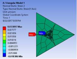
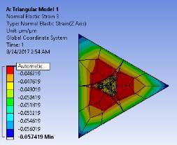
Figure 5.3 Distribution of Normal Elastic Strains on Triangular Model 1 in Transversal and Longitudinal directions

Here, it is clear that, in the strains the transversal directions grow with a considerable difference but in axial direction, they almost remain constant since it is a linearly elastic model.

Distribution of stresses and strains due to compression on all the three triangular models are tabulated below.

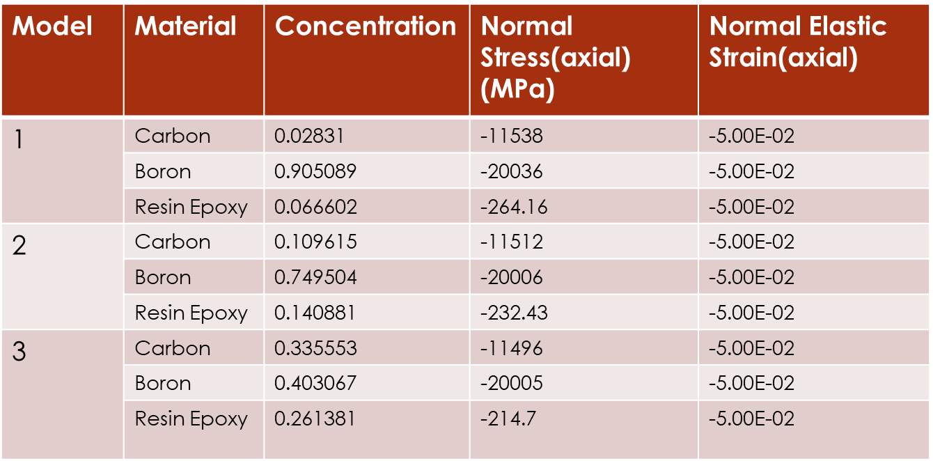
Table 5.1 Table with Normal Stresses and Normal Strains based on the concentration of fibers and matrix for all the Triangular Models

Taking these values into consideration, the longitudinal properties were determined by numerical computations. The calculated results were then compared to the theoretical ones.

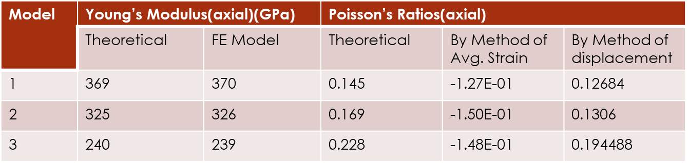
Table 5.2 Comparison of Theoretical and FE Model values of Young’s modulus and Poisson’s Ratio in axial direction for all the three Triangular Models

From the table, it can be concluded that, the results from the Finite Element Analysis of the model are close enough to the theoretical values, which means that the model has good longitudinal properties. Bar graphs are plotted for the same.

Theoretical Results:

Following plots demonstrate the theoretical results of the longitudinal and transversal properties for Triangular Model 1.

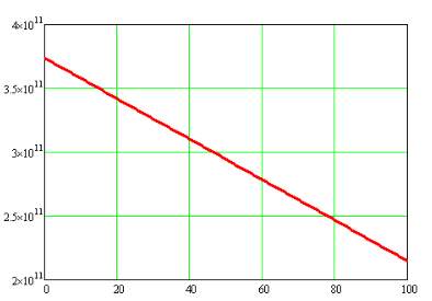
Figure 5.4 Plot between Total Concentration of Fibers and Young’s Modulus in Longitudinal Direction

So, it can be deduced that, with the increase in concentration of fibers, the Young’s Modulus is gradually decreasing. This graph shows the dependency of elastic strain on concentration of fibers.

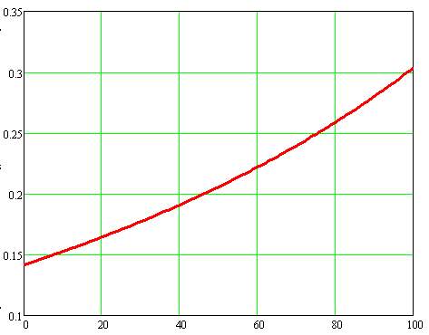
Figure 5.5 Plot between Total Concentration of Fibers and Poisson’s Ratio in Longitudinal Direction

The Poisson’s ratio keeps on increasing with the increase in the total concentration of fibers.

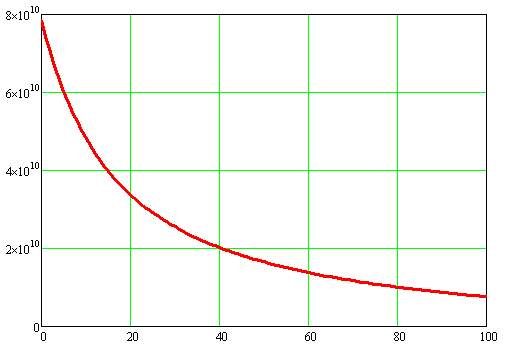
Figure 5.6 Plot between Total Concentration of Fibers and Young’s Modulus in Transversal Direction

From the graph, it is observed that, with the increase in concentration of fibers, the Young’s Modulus decreases drastically.

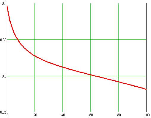
Figure 5.7 Plot between Total Concentration of Fibers and Poisson’s Ratio in Transversal Direction

Here, it can be derived from the graph that, with the increase in the concentration of fibers, there is a gradual decrease in the Poisson’s ratio.

5.1.2 Behavior of Elastic Strain on Infinite Lengths

The variation of elastic strains also depends upon the length of the bar considered. Among the two models, one was of  2000µm in length and the other one was 4000 µm which is double the length of the first model. For the first model, there was a considerable difference between the strains whereas for the second model, the difference between the strains was negligible, which means that as the length of the model tends to infinity, the effect of elastic strains reduces and eventually becomes constant. The simulation  models are shown below with the strain values.

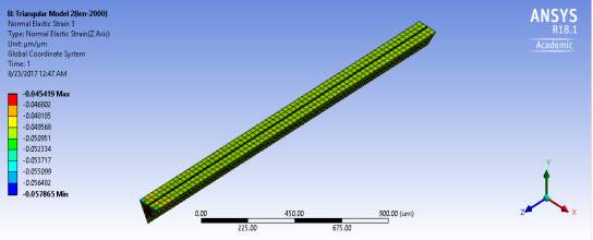Figure 5.8 Normal Elastic Strain of Triangular Model 1 in Axial Direction

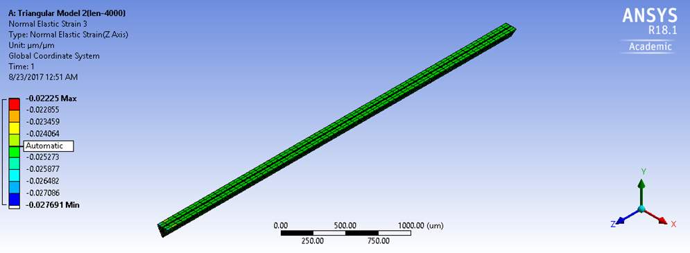
Figure 5.9 Normal Elastic Strain of Triangular Model 1 increased to length 4000µm in Axial Direction

5.1.3 Estimation of Transversal Properties

Some numerical computations were performed to calculate the transversal properties. First the bulk modulus was found based on the pressure applied on the lateral surfaces and this bulk modulus was used to calculate the Young’s modulus and Poisson’s Ratio.

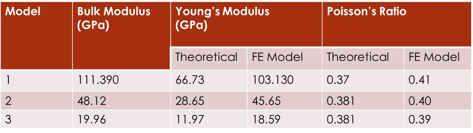
Table 5.3 Comparison of Theoretical and FE Model values of Young’s modulus and Poisson’s Ratio in Transversal Direction for all the three Triangular Models

5.2 Results of Rectangular Models

5.2.1 Estimation of Longitudinal Shear Stiffness

By applying pressure in the longitudinal direction, the deformations in the axial directions were drawn. The deformations at the fixed supports were found to be maximum and the minimum deformations occurred at the ends. This was because there were no forces applied on the side faces of the bar and the bar was restricted to move in all the three directions.

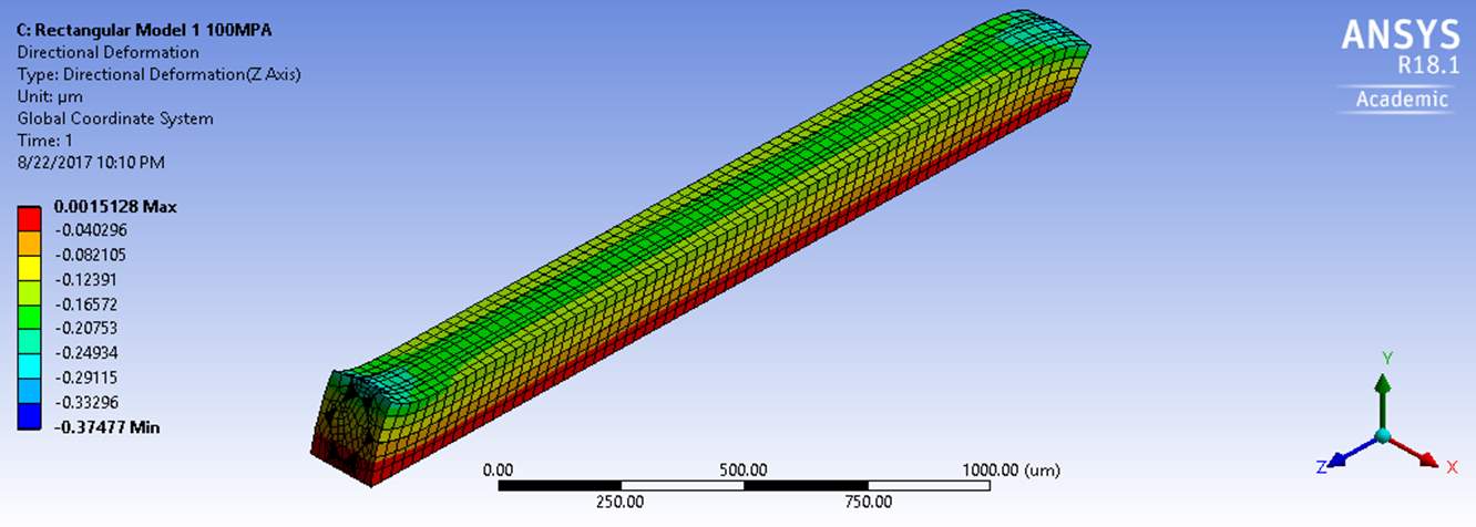
Figure 5.10 Deformation of Rectangular Model 1 subjected to Longitudinal Shear force

Also, the surface displacements were recorded since these were used to calculate the shear modulus. A set of values were taken from the surface using probe and by averaging them the shear modulus was computed.

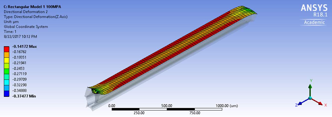
Figure 5.11 Surface Displacements of Rectangular Model 1 subjected to Longitudinal Shear force

5.2.2 Estimation of Transversal Shear Stiffness

Since, the pressure was applied in the transversal direction, the deformation resulted in a skewed body wherein the skew angle could have been measured to calculate the shear angle.

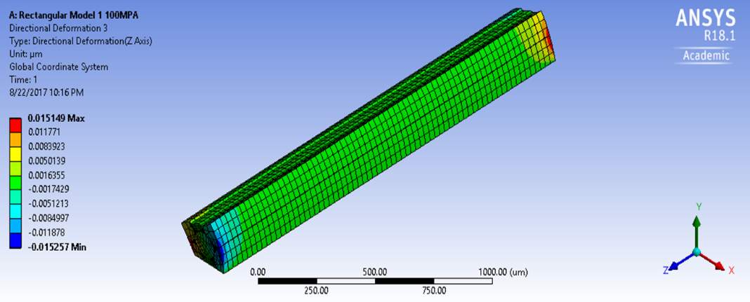
Figure 5.12 Deformation of Rectangular Model 1 subjected to Transversal Shear force

The average of the displacements were taken from the top surface to calculate the shear modulus by probing technique. Below figure indicates the surface deformation.

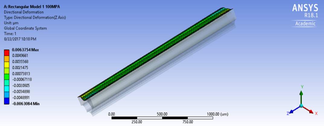
Figure 5.13 Surface Displacements of Rectangular Model 1 subjected to Transversal Shear force

On tabulating the results, it was found that there was a considerable variation in the shear modulus between the theoretical and FE model in the axial direction. On the other hand, there was a huge variation in the transversal shear modulus.

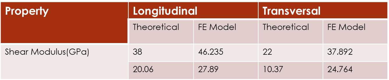
Table 5.4 Comparison of Theoretical and FE Model values of Shear Modulus in Longitudinal and Transversal Direction for Rectangular Model 1 and 2

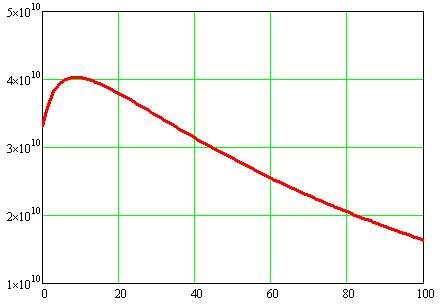
Figure 5.14 Plot between Total Concentration of Fibers and Shear Modulus in Longitudinal Direction

It can be inferred from the graph that, shear modulus increases till the concentration of fibers is 15% and decreases gradually thereafter.

Figure 5.15 Plot between Total Concentration of Fibers and Shear Modulus in Transversal Direction

This graph shows a rapid decrease in the shear modulus till the concentration of 30% and a gradual decrease thereafter.

Chapter 6

SUMMARY AND CONCLUSION

The experiment on Finite Element Model based on the prescribed loads acting on the cell gave results close to theoretical ones, where loads distribution acting on the cell is not prescribed but calculated from known loads applied to the infinite ensemble of the cells.

It can therefore be deduced that Finite Element Method can be applied to more complicated geometries to find compressive strength due to buckling of fibers.

FUTURE WORK

Compressive strength of hybrid composites inside polymer matrix can be investigated further due to buckling of fibers. Because the tensile and compressive strengths of unidirectional fiber reinforced plastics are significantly different, the eddying of boron fibers can support carbon fibers preventing them from buckling.

Finding the optimal combination of carbon and boron fibers is the ultimate goal. The presented work was the first step on this part.

REFERENCES

[1] Peters, S. T. (Ed.). (2013). Handbook of composites. Springer Science & Business Media.

[2] Jones, R. M. (1998). Mechanics of composite materials. CRC press.

[3] Matthews, F. L., & Rawlings, R. D. (1999). Composite materials: engineering and science. Elsevier.

[4] Daryl L. Logan (2011). A first course in the finite element method. Cengage Learning. ISBN 978-0495668251.

[5]  Reddy, J.N. (2006). An Introduction to the Finite Element Method (Third ed.). McGraw-Hill. ISBN 9780071267618.

[6] Bandaru, A. K., Ahmad, S., & Bhatnagar, N. (2017). Ballistic performance of hybrid thermoplastic composite armors reinforced with Kevlar and basalt fabrics. Composites Part A: Applied Science and Manufacturing, 97, 151-165.

[7] Swolfs, Y., McMeeking, R. M., Rajan, V. P., Zok, F. W., Verpoest, I., & Gorbatikh, L. (2015). Global load-sharing model for unidirectional hybrid fibre-reinforced composites. Journal of the Mechanics and Physics of Solids, 84, 380-394.

[8] Dai, G., & Mishnaevsky, L. (2014). Fatigue of hybrid glass/carbon composites: 3D computational studies. Composites Science and Technology, 94, 71-79.

[9] Pandya, K. S., Pothnis, J. R., Ravikumar, G., & Naik, N. K. (2013). Ballistic impact behavior of hybrid composites. Materials & Design, 44, 128-135.

[10] Muhi, R. J., Najim, F., & de Moura, M. F. (2009). The effect of hybridization on the GFRP behavior under high velocity impact. Composites Part B: Engineering, 40(8), 798-803.

[11] Ross, A. (2006). Basalt fibers: Alternative to glass?. Composites Technology, 12(4).

[12] Deák, T., & Czigány, T. (2009). Chemical composition and mechanical properties of basalt and glass fibers: a comparison. Textile Research Journal, 79(7), 645-651.

[13] Sarasini, F., Tirillò, J., Ferrante, L., Valente, M., Valente, T., Lampani, L., … & Sorrentino, L. (2014). Drop-weight impact behaviour of woven hybrid basalt–carbon/epoxy composites. Composites Part B: Engineering, 59, 204-220.

[14] Sarasini, F., Tirillò, J., Valente, M., Ferrante, L., Cioffi, S., Iannace, S., & Sorrentino, L. (2013). Hybrid composites based on aramid and basalt woven fabrics: Impact damage modes and residual flexural properties. Materials & Design, 49, 290-302.

[15] Sarasini, F., Tirillò, J., Valente, M., Valente, T., Cioffi, S., Iannace, S., & Sorrentino, L. (2013). Effect of basalt fiber hybridization on the impact behavior under low impact velocity of glass/basalt woven fabric/epoxy resin composites. Composites Part A: Applied Science and Manufacturing, 47, 109-123.

[16] Tirillò, J., Ferrante, L., Sarasini, F., Lampani, L., Barbero, E., Sánchez-Sáez, S., & Gaudenzi, P. (2017). High velocity impact behaviour of hybrid basalt-carbon/epoxy composites. Composite Structures, 168, 305-312.

[17] Zhu, D., Chen, G., Wu, G., Kang, P., & Ding, W. (2009). Hypervelocity impact damage to Ti–6Al–4V meshes reinforced Al–6Mg alloy matrix composites. Materials Science and Engineering: A, 500(1), 43-46.

[18] Robinson, J. H., & Nolen, A. M. (1995). An investigation of metal matrix composites as shields for hypervelocity orbital debris impacts. International journal of impact engineering, 17(4-6), 685-696.

[19] Zhu, D., Chen, Q., & Ma, Z. (2015). Impact behavior and damage characteristics of hybrid composites reinforced by Ti fibers and M40 fibers. Materials & Design, 76, 196-201.

[20] Meier, U. (2000). Composite materials in bridge repair. Applied Composite Materials, 7(2), 75-94.

[21] Meier, U. (2012). Carbon fiber reinforced polymer cables: Why? Why not? What if?. Arabian Journal for Science and Engineering, 37(2), 399-411.

[22] Naito, K., & Oguma, H. (2017). Tensile properties of novel carbon/glass hybrid thermoplastic composite rods. Composite Structures, 161, 23-31.

BIOGRAPHICAL INFORMATION

Nemani Amruta Rupa earned her Bachelor’s degree in Mechanical Engineering from Jawaharlal Nehru Technological University, Hyderabad, India in 2014. She started her career as a Systems Engineer at Infosys Limited in 2015. Later, in 2016, she joined the University of Texas at Arlington, USA, for her Master’s in Mechanical Engineering. She then started her research work with Dr. Andrey Beyle, and successfully graduated in 2017.

As a Bachelor’s student, she did study project on ‘Manufacturing of gearbox on CNC machine’ from Hindustan Machine Tools Limited, a government of India organization in Hyderabad. In her thesis, she worked on ‘Finite Element Analysis on Hybrid Composites’. She always wanted to work in design and manufacturing sectors.