Discrete Cell Based Model in Fibroblast Cell Migration

1.1      Introduction

1.1.1        Basic cell structure

The basic mammalian eukaryotic cell comprises of a variety of membrane bound structures, cytoplasm and a nucleus. Through the advancement of microscopy techniques, the basic structure and function of these fundamental units of life unfolded. Working inwards, the cell membrane is the outer boundary of the cell consisting of a bilayer of phospholipids. The polarity of this double layer helps to facilitate the cell membranes role of regulating the exchange of substances between the external and internal cellular environments. The membrane surrounds the cytoplasm, which comprises cytosol (gel-like substance) and the organelles. The major organelles suspended within the cytosol are the mitochondria, endoplasmic reticulum (ER) and the Golgi apparatus.  The mitochondria is the powerhouse of the cell and generates energy through a process called oxidative phosphorylation. The ER is a transport network where one of its main functions is to transport newly synthesised proteins to the Golgi apparatus. The Golgi apparatus then completes the process of synthesising the proteins by packaging them in vesicles ready for exocytosis. Finally, the nucleus is a membrane bound organelle responsible for controlling gene expression and replicating DNA during the cell cycle. A cytoskeleton is also present in all mammalian cells. The cytoskeleton acts to maintain cell shape, anchor organelles in place and provide mechanical resistance to deformation ¹.

1.1.2        Cytoskeleton

There are three cytoskeletal systems in mammalian cells: the actin cytoskeleton, the intermediate filament network and microtubules; all of which are involved in the regulation of cell motility. All three networks are interconnected and they are anchored at cell-ECM adhesions and at cell-cell junctions, providing the cell body with mechanical support ². The complexity of the cytoskeleton and its associated proteins has become clear through the advancement of molecular techniques. For example, it is widely understood that the cytoskeleton provides a structural framework for the cell, determining cell shape and cytoplasmic organisation, as well as being responsible for cell movements and internal transportation of organelles and other structures within the cytoplasm (Figure 3-1). In addition, disorganisation of the cytoskeleton has been associated with many pathological conditions, including cancer and cardiovascular diseases ³. Therefore, understanding more about the mechanisms within the cytoskeleton will promote a further understanding of the mechanism of disease within particular pathological conditions.

1.1.2.1        The actin cytoskeleton

The actin monomer (G-actin) is the basic building block of the actin filament (F-actin). Dimers and trimers are formed, through a process called nucleation, and rapid elongation of the filament commences. This elongation is a function of the available G-actin, the most abundant cytoskeleton protein in the mammalian cell ⁴. Put more simply, each G-actin has binding sites that allow head-to-tail with two other G-actin monomers, resulting in polymerisation to form the F-actin filament. F-actin is a polar polymer with a right-handed helical twist ⁵. The polarity stems from the identical orientation of G-actin and is important for further F-actin assembly (elongation) and for establishing a unique direction of myosin movement, relative to actin. This polarity also results in F-actin having two distinguishable ends, called the plus (barbed) and minus (pointed) ends. There is simultaneous assembly and disassembly of G-actin at the plus end and minus end respectively. This process is known as ‘treadmilling’ and is coupled with ATP hydrolysis ⁶.

F-actin plays an important role in epithelial cell cohesion, maintaining the integrity of cellular layers by a ‘belt’ of actin filaments, and in cell migration, as they are found in the plasma membrane protrusion where they form a ‘mesh’. F-actin can also promote edge retraction at the trailing edge of motile cells by converting energy, formed by ATP hydrolysis into tensile force. ATP hydrolysis is used by actin-associated myosin motor proteins to exert force against the stress fibres during muscle contraction ⁶. Actin is essential for the survival of most eukaryotic cells as their filaments provide internal mechanical support, tracks for movement of intracellular materials and force to drive cell movements.

1.1.2.2        The intermediate filament network

Intermediate filaments (IFs) are composed of one or more members of a large family of mainly cytoskeletal proteins. These can be classified into five major types. The first four types (I-IV) are cytoplasmic whereas type V IFs are located within the nucleus. Type I and II are found in epithelial cells and are typically formed from acidic and neutral-basic keratins. Type III IFs are composed of homopolymers of vimentin, typically found in fibroblasts, as well as other cytoskeletal proteins such as desmin, peripheran and glial fibrillary acid protein (GFAP). Type IV and V IFs are expressed in the nervous system and are comprised of internexins and nuclear laminins respectively ⁷. Vimentin IFs preserve mechanical integrity of the cell by contributing to cytoplasmic stiffness and enhancing the elastic properties of the cell, suggesting that IF networks can adapt to mechanical changes in their environment ⁸.

1.1.2.3        The microtubules

The microtubule is a heterodimer of α- and β-tubulin dimers. These tubulin dimers are assembled in a head-to-tail manner culminating in the formation of a protofilament. These protofilaments (typically 13) associate laterally and assemble into tubular microtubule structures. As with the actin polymers, the microtubule is intrinsically polar, with a plus and minus end, due to the organisation of the tubulin dimers in the protofilament. For both F-actin and the microtubule, the plus end grows more rapidly than the minus. The minus end of the microtubule is anchored close to the nucleus of the cell in structures called microtubule organising centres (MTOCs), this is known as a centrosome. Microtubules are responsible for separating chromosomes and for the long-range transport of large particles. Each individual microtubule elongates and shrinks to fulfil a specific role (i.e. chromosome alignment). This phenomenon is termed “dynamic instability” and has long since been a topic of conversation ⁹.

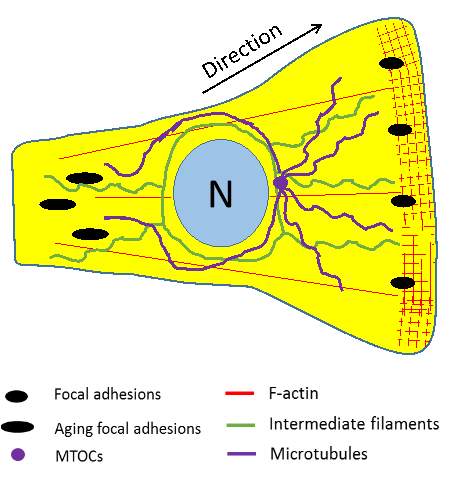Figure 3‑1. Schematic illustration of major cytoskeletal components in motile cells. The cross-hatched region represents the actin framework of the lamellipodia. F-actin is present throughout the cell. Aging focal adhesions in the rear are disassembled to allow retraction. Intermediate filaments surround the nucleus (N), some of which associate with focal adhesions in the lamellipodia. Microtubules are polarised along the direction of migration and accumulate toward the front of the cell.

1.1.3        Role the cytoskeleton plays in cell migration

The ability to migrate is one of the most remarkable properties of animal cells. To date the majority of the research carried out has been conducted on two-dimensional (2-D) surfaces, for experimental convenience. This research has been pivotal in our understanding of how cells migrate. However, a large percentage of cells migrate primarily within a three-dimensional (3-D) environment: during development, specialised cells manoeuvre within the embryo to reach their correct orientation, and in disease, cancer cells migrate from the primary tumour to metastasise secondary sites ¹⁰. In particular, fibroblasts play a crucial role in wound healing by migrating to the wound site and secreting extracellular matrix (ECM) proteins, such as collagen, glycosaminoglycans and glycoproteins, to maintain the structural integrity of the connective tissue ¹¹.

It is generally understood that there are four steps involved in the cycle of cell migration (Figure 3-2) ¹². The first step is the formation of a protrusion, called the lamellipodia, at the front of the cell in response to biochemical and mechanical stimuli. Next, formation of new focal adhesions at the leading edge strengthen the cells attachment to the ECM. Third, increased activity of the actomyosin increases to reduce retraction of the rear. Finally, focal adhesions within the cell rear are dissembled to facilitate the forward movement of the whole cell body ^6,13,14.

The dynamic formation of lamellipodia is regulated by local actin filament assembly and disassembly. During migration, these formations push the cell membrane forward to explore the surrounding environment. Depending on the suitability of the surrounding environment, the cell will either extend further forward or retract. There are two patterns of actin assembly in lamellipodia, branching and elongation, which promote the formation of the actin mesh. Focal adhesion, which are a type of adhesive contact between the cell and ECM, are actively assembled and disassembled in the front and tail of the cell, respectively. At the site of focal adhesion, the extracellular domains of transmembrane integrins connect to the ECM whilst their intracellular tails form attachments to linker proteins, such as vinculin and talin, which in turn bind to the actin cytoskeleton ¹². This chain of connections allow the cell to crawl along the ECM during migration. Subsequently, the triggering of this focal adhesion assembly results in the recruitment of structural proteins (α-actinin, talin, vinculin) and signalling proteins, including focal adhesion kinase (FAK). The structural proteins help to strengthen the attachment to the actin cytoskeleton and the signalling proteins promote further actin polymerisation and other pathways ¹⁵. Further, after the connection between the ECM and actin cytoskeleton has been established, via focal adhesions, external signals induce stress fibre assembly. Stress fibres are contractile bundles containing both F-actin and myosin II filaments. The assembly of these stress fibres generates traction, via the activation of the actomyosin ATPase, propelling the cell forward ^12,16.

IFs have been shown to physically interact with focal contacts in the lamellipodia, raising the possibility that they directly regulate focal adhesion dynamics, and thus cell migration. Cells which express high concentrations of vimentin have been shown to exhibit increased focal adhesion dynamics and destabilised desmosomes, reiterating the impact IFs have on the promotion of cell migration ^17,18. As IFs are widely distributed in the cytoplasm, they have also been shown to regulate cell contraction and nucleus rigidity. In most motile cells, microtubules do not enter the lamellipodia. However, some pioneer cells can extend to the protrusion sites. It is likely that microtubules promote the delivery of vesicles that are essential for cell protrusion. They also promote the polarised delivery of integrns to the leading edge and facilitate the assembly and disassembly of mature focal adhesions within the cells rear, concluding that play a key role in cell protrusion and contraction ¹⁹.

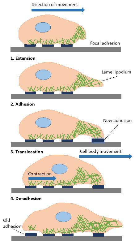Figure 3‑2 Schematic representation of the steps in 2D cell migration. 1. The extension of a lamellapodium. 2. The formation of a new adhesion. 3. The translocation of the cell body. 4. The de-adhesion and retraction at the trailing edge.

1.1.4        The role of mechanotransduction

Mechanotransduction is a process whereby cells can sense their physical surroundings by converting mechanical stimuli into biochemical signals, via the activation of diverse intracellular signalling pathways ²⁰. More work is needed to unravel the complexities of this process. However, it is known that stretch-sensitive ion channels are key regulators of mechanotransduction ²¹. The ECM of connective tissues bear a considerable physical load and provides protection to embedded cells from excessive mechanical forces ²². Fibroblasts, which are abundant in connective tissues, firmly attach to the ECM, via focal adhesions. The link from ECM to the internal architecture of the cell (as previously described), allows the propagation of mechanical forces in both directions. The opposing forces, felt internally and externally by the cell, cancel each other out in stationary cells. However, an imbalance of force in either directions leads to cellular movement ²³. Due to these dynamic interactions, fibroblasts are able to use their adhesion contacts to sense the mechanical properties of the surrounding extracellular environment ²⁴. One of the ways in which fibroblasts gain information about the elasticity of the surrounding ECM is by pulling on an adhesion contact. If there is resistance to the pulling of the fibroblast, this would indicate a stiff ECM and lead to the reinforcement of the focal adhesion site; conversely, any instability detected, via this mechanism, can result in the disassembly of focal adhesions and retraction of the cell ^23,25. Therefore, the importance of understanding the mechanism behind this process is vital as we know that changes in a cells ability to respond to forces are associated with certain disease states, including; muscular dystrophies, cardiomyopathies, cancer progression and metastasis ^20,26.

1.1.5        Replication of Extracellular Matrix (ECM) features

The interaction between a cell and its environment is pivotal for many cellular behaviours such as migration, division, differentiation and proliferation. In vivo, cells depend on an interaction with the 3D scaffold known as ECM. In order to replicate this environment, significant research has focused on the development of cell substrates having both 2D and 3D features that mimic the features of the ECM ^27-29. This has largely been achieved by developing surfaces which have specifically designed features with defined geometries and sizes on a range of different materials. For example, surfaces patterned with micro- and nano-scale grooves ³⁰, pillars ³¹ and pits ³² have been shown to influence cell adhesion ³³ and migration ³⁴ of a range of different cell types.

Although many methods are available for creating and modifying the topography of the patterned surfaces, the most widely used technique involves placing a template mask over the surface that is due to be processed, thereby leaving a predetermined pattern. Such an approach can be seen in lithography-based approaches including; electron beam lithography ^32,35,36, photolithography ^30,37,38 and X-ray lithography ^29,39. The advantages to using these methods are evident in the wide range of well-defined geometries that can be produced on the substrates; however the equipment they utilise is often expensive and time-consuming. A more effective method in the creation of micro-patterned surfaces is laser processing. Laser processing is a quicker, direct-write and flexible process ²⁸. It is also capable of processing relatively large areas by a single exposure. Finally, abrasive polishing methods, which have been largely overlooked, can also develop textured surfaces comparable to those produced by lithography-based methods whilst also being cost-effective. It has been shown that abrasive polishing can produce patterned polyurethane surfaces having ordered, or random, nanoscale features that affect cell adhesion and migration ⁴⁰. Therefore, an abrasive polishing method was chosen to create patterned surfaces for the migration experiments in this chapter.

Machine grinding was used to generate the topographical patterns on the polyurethane surfaces. This method involves the micro-patterning of stainless steel, which can then be used to cast polymer substrates for observing the migration of fibroblasts ⁴⁰. The process was designed to produce features in a ploughed field pattern. However, as there is also a variation in the height and width of the features on each surface, the polymers can be labelled as Linear or Random. An unprocessed plain polymer surface was used as a control and was labelled as ‘Flat’. A previous study has shown that these machine ground surfaces promote adhesion and migration in fibroblast cells compared to unprocessed, flat surfaces ⁴⁰.

1.1.6        Impact of work

This work on mechanotransduction offers great potential into the possibility of controlling cell behaviour, using physical cues. Biofilm formation and the impact of implant integration are some of the key areas that may benefit from this control. Biofilms are communities of adherent cells held together in a self-produced matrix of extracellular polymeric substances (EPS). The formation of biofilms, during infection in wound sites and in inorganic materials such as catheters and stents can be detrimental as they exhibit increased protection from antibiotics ^41,42. Therefore, understanding how to control cellular behaviour by altering its physical environment could provide the platform for a major breakthrough into tackling this complex problem. Equally important, it has been shown that increasing the surface roughness on implants also increases the adhesive properties for fibroblast cells and suggests that there is an improvement in wound healing, limiting the risk of capsular contracture ⁴³.

1.1.7        Mathematical modelling of cell migration

1.1.7.1        Brownian motion

Brownian motion can be described as the random movement of particles in a fluid due to their collisions with other atoms and molecules. This concept is named after Scottish botanist Robert Brown, who in 1827, observed pollen grains moving randomly in the water. However, he was unable to explain the phenomena he had observed and it remained undescribed until 1905, when Albert Einstein published a paper explaining that the fast moving water molecules in the liquid moved the pollen. A modern model of Brownian motion is called the Weiner process. The Weiner process is defined as a continuous-time stochastic process and is named in honour of Norbert Weiner. Brownian motion is considered a Gaussian-Markov process, it has normally distributed random variables over a continuous time constant and is considered a memoryless process ⁴⁴.

In our experiments, it can be difficult to determine whether the cells movement along the patterned surface are due to the cell exhibiting its own motility or due to the cell being subjected to Brownian motion. However, a straightforward approach to distinguishing between Brownian motion and motility is to observe the path of the cell, as Brownian motion tends to appear with more randomness and fluctuations whereas true motility tends to appear with a more biased directed path.

In this chapter, we propose a stochastic mathematical model for the random motility and mechanotransduction of single cells and evaluate the migration paths along the tracks in the patterned surfaces in terms of this model. In our model, the conditions of the cell velocity can be described as a persistent random walk using the Ornstein-Uhlenbeck (O-U) process.

1.1.7.2        Ornstein-Uhlenbeck process

This model allows the simulation of individual cell migration paths. However, the model doesn’t take into account the biochemical and mechanical changes a cell undergoes in order to facilitate movement. Nevertheless, observation of the cell migration experiments reveals comparable random walk-like behaviour, suggesting that it can be described by a related stochastic mathematical equation. Correspondingly, the O-U process has previously been proposed to quantify individual cell random motility. By incorporating a discretedescription of the O-U process, Dunn and Brown were able to successfully demonstrate that this process successfully characterizes fibroblast random motility through use of the autocorrelation functions of cell displacements during discrete time intervals ⁴⁵. Their results support the use of the O-U process as a model of cell motility.

Using the O-U process, the velocity of a cell can be described in terms of two processes: stochastic fluctuations in velocity and deterministic resistance to the current velocity. The stochastic term represents speed and direction of the cell and encompasses all of the probabilistic processes that might affect cell velocity (e.g. response mechanisms to gradient of the cell surface features). The deterministic term affects the persistence of motion through reduction of the cell velocity to zero.

This approach was extended by Stokes et al. ⁴⁶: first by using a continuous version of the O-U process; and second, by adding a term to represent directional bias in response to the presence of a chemoattractant gradient. In the present work, we adapt the directional bias term to represent an environmental gradient instead of a chemical gradient.  We apply our extended model to analyse experimental data of migrating lung fibroblast (LL24) cells on three different surface types with varying features (Flat, Linear and Random).

We begin by describing the continuous version of the O-U process with our adapted directional bias extension that provides a description of haptotaxis. Analysis of the statistical properties of this process reveal two parameters which are explicitly related to two average cell movement quantities, speed (S) and persistence time in velocity (P­_v). These parameters are α and β and represent random fluctuations and velocity decay, respectively. Our model’s applicability is validated for random fibroblast migration and provides us with measurements for α and β. Lastly, an additional parameter, κ, is introduced to account for directed motion of the fibroblast cell in response to a haptotactic gradient. Κ could not be measured directly but we show that we can estimate a value using model generated cell paths.

1.1.8        Chapter aims

1.2      Materials and Methods

1.2.1        Preparation of stainless steel moulds

All patterned surfaces were generated upon a biocompatible polyurethane polymer (described in Section 1.2.4). Patterns were developed on the polymer indirectly, by casting off the flat end surface of a cylindrical stainless steel mould that had been cut from stainless steel rods (grade 316, cylinder height 13 mm, diameter 18 mm). To prepare the stainless steel moulds for patterning, their flat surfaces were first polished to remove all marks caused by the cutting process. This was achieved using a METASERV universal polisher and silicon carbide sheets of decreasing grit size (60 to 1200 B) followed by a polishing cloth. This resulted in the stainless steel cylinder having a mirrored surface finish (mean Ra value of approximately 0.02 μm) which could then be used for processing.

1.2.2        Laser patterned surface development

The experiments were performed using an SPI solid state pulsed fibre laser system (G3.0 20WPulsed Fibre Laser HS Series) with a maximum mean laser power (P) of 20 W, wavelength (λ) of 1064 nm and variable pulse duration (τ) of 9–200 ns. The laser beam was collimated and expanded up to 10mmthrough a 5× beam expander. The expanded beam was then propagated to a galvanometer (scanning head, GSI Lightning), which consists of two mirrors that control the laser beam path across the work piece. A translational x-y-z table (Aerotech Inc., UK) was used to accurately position the sample at the focal position of the processing lens. The reflected beam was then focused using a

100 mm focal length lens (Linos F-Theta-Ronar 1064 nm + VIS) which produced a focused spot size of 30 μm in diameter. The pattern was generated over an 8mm2 area. The laser spot was focused onto the stainless steel and programmed to scan in a raster pattern across the surface with a line spacing of 50 μm between each pass. The parameters used for processing were: laser power 4 W, pulse duration 9 ns, frequency 25 kHz, a processing speed of 500 mms−1 and pass number 20. These parameters resulted in the stainless steel having a grooved surface with features on the micron scale.

1.2.3        Abrasive patterned surface development

Once polished to achieve an initial mirrored finish (as described above in Section 1.2.1) the stainless steel cylinder was then polished to achieve a topographical surface patternation through the use of abrasive paper (1200 B). By controlling the motion of the stainless steel cylinders relative to the silicon carbide abrasive paper, surfaces having either directional, or random, sub-micron abrasive marks could be produced, termed here as ‘nano-scratches’. The directional (linear) features are a result of the METASEV universal polisher’s spinning motion, while the more random features are the result of manually rubbing the steel mould across the surface in different directions. The surface topography was subsequently characterised by white light interferometry and scanning electron microscopy. These stainless steel cylinders could then be used as master moulds to cast polymer substrates. In total two different patterns were produced; having linear and randomly organised features.

1.2.4        Casting polymer substrates

Casting the polymer over the stainless steel moulds produces an inverted pattern on the polymer surface. Employing this indirect processing method ensures that only the surface topography/roughness of the material is altered and not the material chemistry. The polymer used here was polyurethane and was provided by Biomer Technology Ltd. The polymer substrates were produced using 8% polyurethane in 2:1 Dimethylformamide (DMF) and Tetrehydrofuran (THF). This was poured onto the stainless steel moulds and cured at 60 °C for 2 h. Following this the mould/cast was allowed to cool before peeling off the polymer from the mould following the grain of the pattern. Prior to cell culture all polymer surfaces were sterilised by washing with 70% ethanol then exposing to UV light for 30 min. Finally, the polymers were washed with sterilised distilled H2O.

1.2.5        White light interferometry for surface characterisation

A Bruker Contour GT-K 3D optical microscope equipped with Vision 64 software was used to image the surfaces of the patterned polymers. This enabled feature heights/widths and roughness to be determined. (Figure 1-1).

1.2.6        Cell culture

The cells described in this work are human lung fibroblast cells (LL24) which have been purchased from the European Collection of Animal Cell Cultures (ECACC) UK. Fibroblast cells were chosen because there is extensive evidence showing that fibroblast cells respond to changes in surface topography both in vitro and in vivo. The LL24 cell line was chosen as it is a well characterised, stable, normal human diploid cell line. All cell culture work was carried out under aseptic conditions in a grade II laminar flow cabinet (EBSCO). Cells were maintained at 37 °C in a humidified 5% CO2/95% air atmosphere in Dulbecco’s Modified Eagles Medium(DMEM) (Sigma-Aldrich, D6429) supplemented with 10% foetal bovine serum (Sigma-Aldrich, 0804 ) and 1% penicillin-streptomycin. All experiments were carried out using cells at passage numbers 20–24.

1.2.7        Cell migration assay

To determine if the different surfaces affected cell migration, time-lapse imaging and subsequent cell tracking was performed over a four-hour period using a Zeiss LSM 510 confocal microscope. Briefly, the polymer surfaces were sterilised in 70% ethanol, washed in PBS then placed into 35 mm cell culture dishes. Next 100,000 cell/cm2 were seeded onto the polymer surfaces and the dish was placed into the microscope environmental chamber (S-2, PeCon GmbH, Germany), The chamber was maintained at 37 °C, 5% CO2 in a 60–70% humidified air atmosphere using a Temcontrol 37-2 and CTI-controller 3700 (PeCon GmbH, Germany). Images were taken every 10 min for 2.5 h using a 20× Plan-Apo/0.75 NA DIC objective lens, while scanning using a Helium- Neon (HeNe) laser at 543 nm. Images of the patterned surfaces without any cells seeded on where also taken, so that the specific features of each surface could be transferred to the simulation software for the mathematical model cells to migrate on (Figure 3-3).

1.2.8        Measurement of cell trajectories, mean squared displacement and tortuosity

Cell movement tracks were analysed using ImageJ software (National Institute of Health, NIH) with a manual tracking plugin (Institute Curie, France) used to analyse the data produced from the time-lapse image series. The centroid of the cell area was used to represent the cell position. The time increment between image frames was ten minutes. This was long enough to discern forward cell movement without losing track of the cell’s position. The result was a series of distances with time for each cell. The net displacement was calculated by difference of position at the beginning and end of each time step. The mean square displacement, (D²), was calculated by taking the total mean of each individual cell’s movement for each time point. This resulted in a series of D² values for increasing values of time. Tortuosity, τ, can be defined as the property of a curve being tortuous i.e. having many turns (twisted). Tortuosity can be estimated using the arc-chord ratio: the ratio of the length of the curve (L) to the distance between the ends of it (C).

τ= LC ,                                                                   (3-1)

L is the total curved-line distance and is measured by obtaining the total distance travelled by the fibroblast from t=0 to t-end. C is the straight-line distance travelled by the fibroblast and can be obtained by measuring the distance of the cell’s position at t-end from its origin position at t=0.

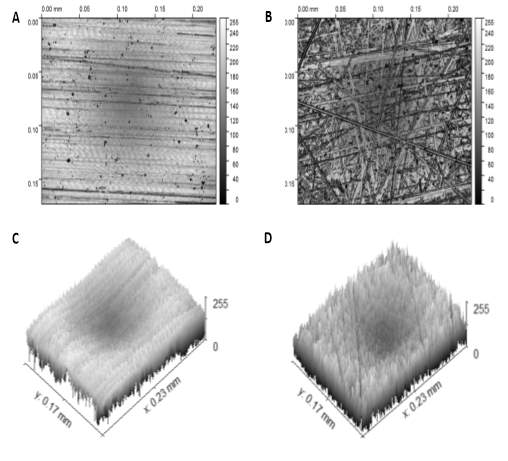Figure 3‑3. Microscope images of patterned surfaces. (A & B) These images show the Linear patterned surface and Random patterned surfaces, respectively. (C & D) These are 3D schematic images of the Linear patterned surface and Random patterned surfaces, respectively.  The scale in the z-axis represents intensity.

1.2.9        Mathematical model

We analyse the cell motility in terms of a stochastic mathematical model. The O-U process is the simplest type of a continuous, random motility model, as it describes a Markov process. This means that only the current state of the cell is taken in to account and the cell’s previous positions have no bearing on future movements; there is no memory to the motion. Although this may seem oversimplified, Dunn and Brown showed that this process is sufficient to describe random motility in fibroblast cells. Initially, this simple stochastic model describes a persistent random walk. However, through the addition of our haptotactic gradient, it becomes a biased random walk model. For this model, we assume that the cell effectively responds to a spatial gradient of focal adhesions between the cellular membrane and the surfaces topography, although we make no assumptions about the cell’s actual underlying mechanism of perception. We also assume that the fibroblast cell moves perpendicular to and ‘uphill’ gradient in the features of the surface i.e. the cell migrates along the surface grooves rather than across them.

We now describe the details of our extended, continuous model. One equation (Equation 3-2) describes the velocity of a single model cell as it evolves with time. A second equation (Equation 3-3) is then used to determine the cell’s (x, y) position from its velocity, producing a calculated trajectory for the model cell. From these equations, the mean squared displacement and tortuosity with the model characteristics can be calculated. Comparison of these predicted metrics to those obtained experimentally will allow us to: (1) examine the validity of the model and (2) determine values of the model parameters, α and β, for the fibroblast migration.

The rate of change of cell velocity in our model is the sum of three components: the first two components represent the random motility behaviour, and the third represents the haptotactic, or directed, behaviour. For random motility, the first term describes the deterministic resistance to the cell’s motion, and the second represents the random accelerations (or fluctuations) of the movement. The third component that describes the haptotactic behaviour provides a directional bias in the presence of a patterned surface gradient. Mathematically, these three components are summed to give the following stochastic differential equation for the rate of change of the cell velocity, Ṽ:

dṼt= -βṼtdt+ αdW̃t+ Ψ̃tdt,                                (3-2)

change in velocity = resistance to motion + random fluctuations + haptotactic bias,

where α and β are the motility parameters, t is time,

W̃is the vector Weiner process (white noise), and

Ψ̃is the drift function, which describes the effect of the surface features on the velocity of the cell. The equation for describing

Ψ̃is derived below (Equation 3-4). The variables V,

Ψ̃and W have velocity that occurs in more than one dimension, as indicated by the tildes (~) over them. As the velocity of the cell is a rate of change of the cell’s position, the position of the cell,

x̃, can be obtained by integrating the velocity with time:

x̃t= ∫0tṼt’dt’.                                               (3-3)

We can see from Equation 3-2 that for the velocity process to describe random motility, the drift function must be equal to zero. Therefore, it can be confirmed that random motility is characterised by α and β. We can view β as the magnitude of resistance to motion, leading to a decrease in the persistence of velocity as β increases.

The drift function provides the directional bias in velocity caused by a cell reacting to the presence of mechanical stimuli. As previously mentioned, we assume that the cell effectively responds to a spatial gradient of focal adhesions between the surfaces of the cell and surrounding environment. The gradient will be dependent on the steepness of the surrounding pattern features. The simplest way to incorporate this is to let the drift function be proportional to

cos-1⁡θ, where θ is the angle between the direction of the cell and the direction of the surface pattern with the steepest gradient. Thus, introducing κ as the proportionality constant gives:

Ψ̃= κ∇acos-1⁡θ,                                              (3-4)

drift function = haptotactic responsiveness × attractant gradient size × orientation in gradient

Equations (3-2) and (3-4) provide a description of the velocity process of a single cell moving with the average properties represented by the random motility parameters αand βand the haptotaxis parameter κ. Each cell described by equation (3-2) with a given set of parameters, α, β and κ, has a different path or trajectory (owing to different realisations of the random noise process,

W̃) but the same ‘degree’ of randomness, velocity decay rate constant, and sensitivity to attractant gradients. Thus, our modified O-U process provides a quantitative framework in which to interpret fibroblast cell motility. For this framework to be meaningful, we must first demonstrate that it is a valid description of actual cell trajectories. If shown, we can utilise this framework to obtain values for the parameters α, β and κ, which then provide a quantitative description of the characteristics of the actual cell’s intrinsic motility properties on the different polyurethane surfaces.

1.3      Results

1.3.1        Cell trajectories

Several typical cell paths for random fibroblast cell migration are shown in Figure 3-4A. The paths reveal that fibroblast cell migration travel with a combination of smooth and twisted trajectories. The persistence time in a given direction does not appear to be very long. The duration of all cell paths obtained ranged from 140-160 minutes. The final measurement of the cell path is represented by the round head feature of the trace (—•), whereas the origin of the cell trajectory is represented by the tail like feature (—).  The cells that moved off screen were ignored in this study. The cell paths for fibroblast cell migration on the Linear and Random patterned surfaces are shown in Figure 3-4B and Figure 3-4C, respectively. These paths represent the movement of the centroid of the cell area. Qualitatively, directional changes in the cell paths appear smooth initially, before more frequent turns in trajectory. Certainly, it can be suggested that the fibroblast cells on the linear pattern (Figure 3-4B) travel a greater distance from their origin site compared to the cells on the other polyurethane surfaces. Nevertheless, more significant conclusions are needed to describe the cell trajectories which can be drawn from the quantitative data extracted from the experiments.

1.3.2        Experimental metrics

Firstly, the tortuosity was calculated for collective cell migration on each of the three surfaces (Flat, Linear and Random).  These values are plotted in a bar chart with error bars for comparison in Figure 3-5A. In turn, the tortuosity measured for each surface was 3.42, 2.95 and 2.96. For reference, if a cell were to have a tortuosity ratio equal to 1, that cell path would have a trajectory in a perfect straight line.  There is a large variance in tortuosity for individual cell migration on the flat and random surface, compared to that off the linear surface. This suggests that there is a greater persistence time in cell direction for fibroblast cells migrating on a surface with linear features (ANOVA needed). What is also evident from the values outputted from these measurements, is the suggestion that the cells have a more directed migration on the surfaces containing the nano-scratch features i.e. have a lower tortuosity value indicating greater straight line movement.

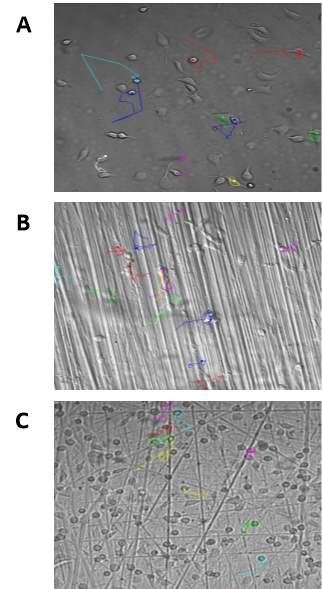Figure 3‑4. Tracking of cell migration on the polyurethane surfaces. Image showing the migratory paths of fibroblast cells on the Flat surface (A), Linear surface (B) and Random surface (C). T = 150min.

The mean curve- and straight-line distances for the migration of the fibroblast cell populations on each surface was also plotted in a bar chart (Figure 3-5B). The flat surface had a mean curve-line distance of 105 μm and straight-line distance of 34 μm. Similarly, the mean curve-line distance travelled by the cell population on the random surface was 99 μm with a straight-line distance of 37 μm. Contrastingly, the distances travelled by the fibroblast cells on the linear surface were much greater. The mean curve-line distance and straight-line distance measured for this surface were 157 μm and 63 μm, respectively. Again, as with the tortuosity measurements, there is a smaller variance in individual cell distance travelled along the linear surface compared to the other surfaces, particularly for the curve-line metric.

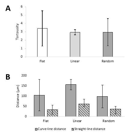Figure 3‑5. Experimental metrics from cell migration experiments. Column chart showing the tortuosity (A) and distances travelled (B) by the fibroblast cells on each polyurethane surface.

In Figure 3-6, the mean squared displacement (D²), is plotted against time. The time course of the experiments varies between 130-160 minutes. This is due to the initial frames of certain time-lapse videos having fibroblast cells still in the attachment phase of the experiment. D² measures the deviation of the position of a cell with respect to a reference position over time, and is useful in determining if the movement of a cell is solely down to diffusivity or if an external force is directing the motion. For comparison of the D² measurements, with respect to the patterned surface they journeyed, we examine the t-end results. The t-end D² for the flat surface was 1076 μm², the linear surface was 2367 μm² and the random surface was 1326 μm². There is high variance in all 3 results, which is to be expected when taking the mean of individual cell migration paths from differing starting points on non-uniform surfaces i.e. different feature depths. Once more, it is clear to see that cell migration on the linear surface is much greater with approximately twice as much displacement compared with the flat and random surfaces. This is more clearly seen in Figure 3-6D. For the initial time frames, the linear and random trajectories are almost identical, suggesting that the movement could be directed as they attach to the pattern features. However, as the time increment increases, the random trajectory more resembles the flat trajectory, which is more typical of random motility. This would be expected with the random pattern having features for the fibroblast to transverse in all directions.

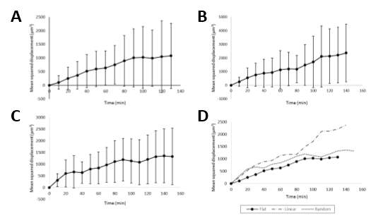Figure 3‑6. Experimental mean squared displacement results. Examples of experimental mean squared displacement (D²) as a function of the time increment for all the migrating cells on the flat (A), linear (B) and random (C) patterned surfaces. (D) All D² measurements are plotted on the same graph with legend indicating which trace belongs to which surface.

1.3.3        Applicability of model for random motility

The first level of validation of the model is to show that related average properties produced by the model are the same as those produced by the real cells in the experiments. For our model, the related average properties are the mean squared displacement of the cells, tortuosity, and curve- and straight-line distance. Initially, only the flat surface is modelled using Equation 3-2, without the haptotactic part (

Ψ), and Equation 3-3 to yield an actual cell path for the migrating model cells.

To initialise the model, the positional coordinates of the cells origin were set to (0, 0) and its initial velocity in the x and y directions randomised to have any value ranging from -10 to 10. The time increment, t, was set to match the experimental time with the time increments, dt, being as small as possible. The two random motility parameters, α and β, were initially set as 73.6 and 0.22, respectively, to mimic the mean values obtained in the continuous model designed by Stokes et al. ⁴⁶. These parameters are to be more accurately determined based on the experimental metrics later. Once initialised, the cells velocity and position were updated using Equations 3-2 and 3-3 for the duration of the time course. The velocity and position of the cell were plotted (Figure 3-7) as well as the simulated trajectory of the model cells (Figure 3-8). Finally, the average properties were produced and the mean squared displacement for the model simulation plotted.

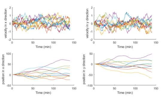Figure 3‑7. Cell velocity and position in x and y position over time. Graphs showing the simulated positions and velocities on both axis for multiple migratory model cells for the flat surface simulation.

In Figure 3-7, the velocity changes in both axes are plotted. The influence of the α parameter is evident by the fluctuations observed in the traces. If this parameter were to be set to zero, the deterministic parameter, β, would produce traces showing the velocity revert to zero over time. These initial traces provide confidence that the model simulates random motility. This is further backed up when the trajectories of all the simulated model cells are plotted together (Figure 3-8). The origin of each cell is exactly same. However, each trajectory sets off in a separate direction with multiple twists in each path, highlighting the effect of the randomness encoded from the equations.

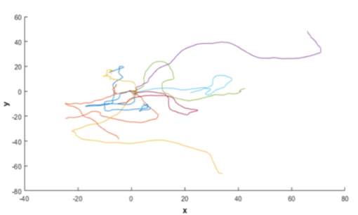Figure 3‑8. Simulation of cell migration path using MATLAB. Example of the simulated cell paths for the flat surface. Parameter κ not included in calculation of trajectory.

1.3.4        Determination of random motility parameters

Now that we have a working model of random motility, we can optimise the parameters, α and β, to find values that best describe the behaviour of the system we are describing. In this instance, the system we are describing is that of fibroblast migration. As we already have experimentally derived metrics from this system, those values can be used for parameter estimation and produce a function of best fit for our data points. To begin, we run our simulation model for random motility again, whilst varying α and β each time (100 x 100 runs). This will result in a tortuosity, curve-line distance, straight-line distance and D² value for each individual combination of α and β (Figure 3-9). The range of α and β values were plotted against each other with the metrics plotted on the z-axis. This gives a visual representation of which α and β combinations would be most suitable for describing are experiments. To aid in this visualisation, a contour plot was added (white line). This contour plot represents the corresponding experimentally derived metric from the fibroblast migration experiments on the flat surface. Therefore, any α and β combination falling on this line can be assumed to be the most appropriate combination to describe our experiments.

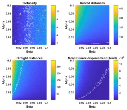Figure 3‑9. Parameterisation of alpha and beta. Plots show a range of dimensionless alpha and beta values (0 – 0.1) with tortuosity, curved line distance, straight line distance and the t-end mean squared displacement value plotted on the z-axis, respectively. The white contours represent the experimentally derived values for tortuosity, curved line distance, straight line distance and the t-end mean squared displacement for the flat surface. The alpha and beta values on these lines are deemed most appropriate for the simulated experiments.

Another test for goodness of fit is the chi-squared (χ²) distribution. The chi-squared distribution is used in the common chi-squared test for goodness of fit of an observed distribution to a theoretical one. Moreover, this test establishes whether an observed frequency distribution differs from a theoretical one. The chi-squared values for tortuosity, curve-line distance, straight-line distance and mean squared displacement were calculated using Equation 3-5:

χ2= ∑i=1nSi-Ei2Ei,                                                (3-5)

where S is the simulated measurement of the metric and E is the experimentally derived measurement of the metric. In our model, χ² values were calculated for each of the flat surface metrics and these values were used to generate plots to help determine the optimal value of α and β (Figure 3-10). Similar to Figure 3-9, the chi-squared values for each of the metrics are plotted against the range of α and β values (Figure 3-10A). To find a combination of α and β values that will give a good fit of all four metrics simultaneously, their respective chi-squared values were totalled and plotted against α and β (Figure 3-10B). This plot shows that lower values of α and β give the best fits for the experiment. Figure 3-10C shows a plot of the individual experimental values against the range of α and β values. Ideally, the optimal value of α and β would be chosen by finding the point at which all four metrics crossover on the plot. However, there is no point of crossover on the plot for the curve-line (red trace) and the straight-line (black) distances. In fact, the tortuosity metric (blue trace) is the only result that has any crossover. Therefore, the total chi-squared values were plotted against the range of α and β values in combination with a curve fitting tool (Figure 3-10D). A function was used to fit a polynomial to the data. Specifically, a quadratic, or second degree polynomial, was used. Therefore, any combination of α and β that falls on the plot in Figure 3-10D is appropriate for describing out experiment and for use in the subsequent simulations for the linear and random surfaces. For these simulations, we use α = 0.01 and β = 0.03.

Figure 3‑10. Chi-squared plots.

1.3.5        Determination of haptotactic responsiveness

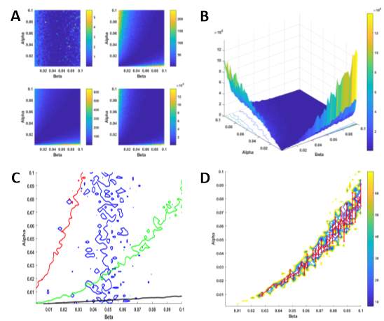
Before estimation of the dimensionless haptotactic responsiveness can be accomplished, the polyurethane surface patterns and features need to be encoded in the model. This was achieved by taking the microscope image data, from Figure 3-3, saving it as an ASCII-delimited file and using the MATLAB function ‘dlmread’ to convert it into a matrix. This matrix now contains numerical values which represent intensity values between 0 and 255 for each point of the image (Figure 3-11). These intensity values were subsequently converted into gradient values for each x-y coordinate. This allowed the steepness of the actual features present on the experimental polymers to be incorporated into the simulations. The initialisation and time parameter set up is the same as it was for the flat model simulations and α = 0.01 and β = 0.03. Cell velocity is updated using Equation 3-2 with the drift function, derived from Equation 3-4, added this time and the cell position is updated using Equation 3-3. For Equation 3-4,

∇ais represented by the gradient calculated from the microscopy data, θ is calculated by taking the inverse cosine of the dot product at each cell position and κ is initially inputted as a random value between 0 and 1. In Euclidean geometry, the dot product of two Euclidean vectors, possessing both magnitude and direction, a and b can be defined by Equation 3-6:

a∙b= abcos⁡θ,                                            (3-5)

where θ is the angle between a and b.

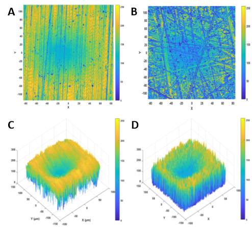Figure 3‑11. Simulated images of microscope data produced by MATLAB. The microscope image data (previously shown in Figure 3-1) was read into MATLAB to produce simulated images for the in-silico cells to move on. As before, there are 2D images of Linear (A) and Random (B) and 3D images of Linear (C) and Random (D). The z-axis represents intensity.

As before we can use our experimental metric to optimise and determine the haptotactic responsiveness parameter, κ. (Will add in this section once I obtain figures from MATLAB). We can now simulate our models representing the linear and random patterned surface experiments. As with the random motility model, we can plot the model cell migration paths derived from our simulations (Figure 3-12). It is evident that the cell migration paths from the linear and random surface models appear to exhibit features associated with a biased-walk model rather than a random-walk model. The cell trajectories are less twisted with more persistent crawling in a single direction. In particular, the cell trajectories for the random simulation show a preference for the larger features present on the surface. This suggests that we have successfully created a biased-walk model. In addition to the cell trajectories, the simulated mean squared displacement values were also plotted (Figure 3-13). Comparison of the experimental mean squared displacement graphs in Figure 3-6 show a strong correlation with the simulated plots from our model. Quantitatively, by looking at the t-end values from both sets of graphs (Table 3-1), it can again be shown that our continuous, extended model represents what occurs experimentally relatively accurately.

	Experimental D2 (μm2)	Simulated D2 (μm2)
Flat	1076	~1800
Linear	2367	~2600
Random	1326	~1700

Table 3‑1. T-end mean square displacement values.

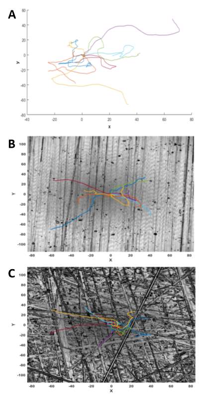Figure 3‑12. Simulation of cell migration paths using MATLAB. Example of simulated cell paths for Flat (A), Linear (B) and Random (C) surfaces. All simulations had a starting point of (0, 0). Gradient and chemotactic responsiveness (κ) values were included in simulations B and C.

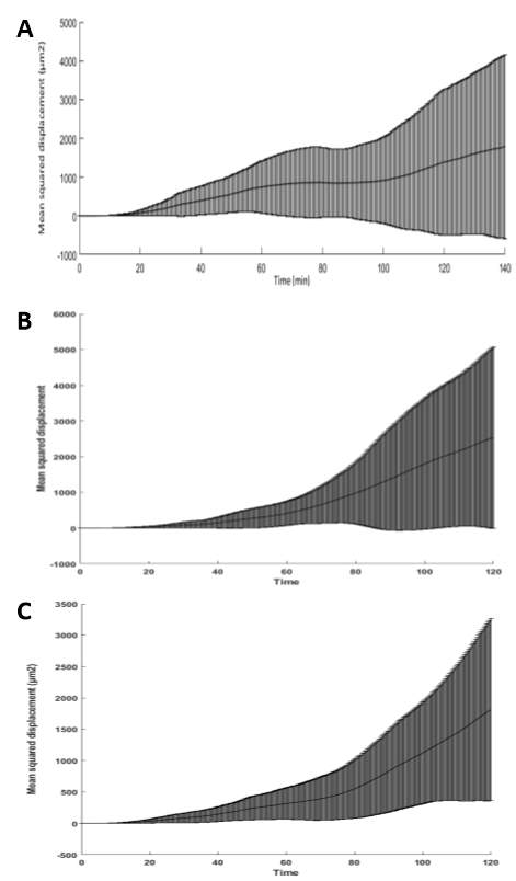Figure 3‑13. Simulated mean squared displacement results. Examples of simulated mean squared displacement (D²) as a function of time increment for all the migrating cells on the Flat (A), Linear (B) and Random (C) patterned surfaces.

1.4      Discussion

• Which pattern promotes adhesion/migration?
• How does the model weigh up?

1.5      References

1. Nicolson GL. Cell membrane fluid-mosaic structure and cancer metastasis. Cancer Res. 2015;75(7):1169-1176. doi: 10.1158/0008-5472.CAN-14-3216 [doi].

2. Li S, Huang NF, Hsu S. Mechanotransduction in endothelial cell migration. J Cell Biochem. 2005;96(6):1110-1126. doi: 10.1002/jcb.20614 [doi].

3. Ramaekers FC, Bosman FT. The cytoskeleton and disease. J Pathol. 2004;204(4):351-354. doi: 10.1002/path.1665 [doi].

4. Wegner A, Engel J. Kinetics of the cooperative association of actin to actin filaments. Biophys Chem. 1975;3(3):215-225.

5. Blanchoin L, Boujemaa-Paterski R, Sykes C, Plastino J. Actin dynamics, architecture, and mechanics in cell motility. Physiol Rev. 2014;94(1):235-263. doi: 10.1152/physrev.00018.2013 [doi].

6. Pollard TD, Cooper JA. Actin, a central player in cell shape and movement. Science. 2009;326(5957):1208-1212. doi: 10.1126/science.1175862 [doi].

7. Lowery J, Kuczmarski ER, Herrmann H, Goldman RD. Intermediate filaments play a pivotal role in regulating cell architecture and function. J Biol Chem. 2015;290(28):17145-17153. doi: 10.1074/jbc.R115.640359 [doi].

8. Mendez MG, Restle D, Janmey PA. Vimentin enhances cell elastic behavior and protects against compressive stress. Biophys J. 2014;107(2):314-323. doi: S0006-3495(14)00470-6 [pii].

9. Horio T, Murata T. The role of dynamic instability in microtubule organization. Front Plant Sci. 2014;5:511. doi: 10.3389/fpls.2014.00511 [doi].

10. Friedl P, Gilmour D. Collective cell migration in morphogenesis, regeneration and cancer. Nat Rev Mol Cell Biol. 2009;10(7):445-457. doi: 10.1038/nrm2720 [doi].

11. Martin P. Wound healing–aiming for perfect skin regeneration. Science. 1997;276(5309):75-81.

12. Tang DD, Gerlach BD. The roles and regulation of the actin cytoskeleton, intermediate filaments and microtubules in smooth muscle cell migration. Respir Res. 2017;18(1):54-017-0544-7. doi: 10.1186/s12931-017-0544-7 [doi].

13. Gerthoffer WT. Migration of airway smooth muscle cells. Proc Am Thorac Soc. 2008;5(1):97-105. doi: 5/1/97 [pii].

14. Cleary RA, Wang R, Waqar O, Singer HA, Tang DD. Role of c-abl tyrosine kinase in smooth muscle cell migration. Am J Physiol Cell Physiol. 2014;306(8):C753-61. doi: 10.1152/ajpcell.00327.2013 [doi].

15. Tang DD. Critical role of actin-associated proteins in smooth muscle contraction, cell proliferation, airway hyperresponsiveness and airway remodeling. Respir Res. 2015;16:134-015-0296-1. doi: 10.1186/s12931-015-0296-1 [doi].

16. Murali A, Rajalingam K. Small rho GTPases in the control of cell shape and mobility. Cell Mol Life Sci. 2014;71(9):1703-1721. doi: 10.1007/s00018-013-1519-6 [doi].

17. Leduc C, Etienne-Manneville S. Intermediate filaments in cell migration and invasion: The unusual suspects. Curr Opin Cell Biol. 2015;32:102-112. doi: 10.1016/j.ceb.2015.01.005 [doi].

18. Mendez MG, Kojima S, Goldman RD. Vimentin induces changes in cell shape, motility, and adhesion during the epithelial to mesenchymal transition. FASEB J. 2010;24(6):1838-1851. doi: 10.1096/fj.09-151639 [doi].

19. Etienne-Manneville S. Microtubules in cell migration. Annu Rev Cell Dev Biol. 2013;29:471-499. doi: 10.1146/annurev-cellbio-101011-155711 [doi].

20. Ingber DE. Cellular mechanotransduction: Putting all the pieces together again. FASEB J. 2006;20(7):811-827. doi: 20/7/811 [pii].

21. Martinac B. Mechanosensitive ion channels: Molecules of mechanotransduction. J Cell Sci. 2004;117(Pt 12):2449-2460. doi: 10.1242/jcs.01232 [doi].

22. Guilak F, Alexopoulos LG, Upton ML, et al. The pericellular matrix as a transducer of biomechanical and biochemical signals in articular cartilage. Ann N Y Acad Sci. 2006;1068:498-512. doi: 1068/1/498 [pii].

23. Chiquet M, Gelman L, Lutz R, Maier S. From mechanotransduction to extracellular matrix gene expression in fibroblasts. Biochim Biophys Acta. 2009;1793(5):911-920. doi: 10.1016/j.bbamcr.2009.01.012 [doi].

24. Balaban NQ, Schwarz US, Riveline D, et al. Force and focal adhesion assembly: A close relationship studied using elastic micropatterned substrates. Nat Cell Biol. 2001;3(5):466-472. doi: 10.1038/35074532 [doi].

25. Bershadsky A, Kozlov M, Geiger B. Adhesion-mediated mechanosensitivity: A time to experiment, and a time to theorize. Curr Opin Cell Biol. 2006;18(5):472-481. doi: S0955-0674(06)00123-2 [pii].

26. Wang H, Brennan TA, Russell E, et al. R-spondin 1 promotes vibration-induced bone formation in mouse models of osteoporosis. J Mol Med (Berl). 2013;91(12):1421-1429. doi: 10.1007/s00109-013-1068-3 [doi].

27. Huttenlocher A, Horwitz AR. Integrins in cell migration. Cold Spring Harb Perspect Biol. 2011;3(9):a005074. doi: 10.1101/cshperspect.a005074 [doi].

28. Aguilar CA, Lu Y, Mao S, Chen S. Direct micro-patterning of biodegradable polymers using ultraviolet and femtosecond lasers. Biomaterials. 2005;26(36):7642-7649. doi: S0142-9612(05)00371-6 [pii].

29. Liliensiek SJ, Campbell S, Nealey PF, Murphy CJ. The scale of substratum topographic features modulates proliferation of corneal epithelial cells and corneal fibroblasts. J Biomed Mater Res A. 2006;79(1):185-192. doi: 10.1002/jbm.a.30744 [doi].

30. Reynolds PM, Pedersen RH, Riehle MO, Gadegaard N. A dual gradient assay for the parametric analysis of cell-surface interactions. Small. 2012;8(16):2541-2547. doi: 10.1002/smll.201200235 [doi].

31. Ghibaudo M, Trichet L, Le Digabel J, Richert A, Hersen P, Ladoux B. Substrate topography induces a crossover from 2D to 3D behavior in fibroblast migration. Biophys J. 2009;97(1):357-368. doi: 10.1016/j.bpj.2009.04.024 [doi].

32. Curtis AS, Casey B, Gallagher JO, Pasqui D, Wood MA, Wilkinson CD. Substratum nanotopography and the adhesion of biological cells. are symmetry or regularity of nanotopography important? Biophys Chem. 2001;94(3):275-283. doi: S0301-4622(01)00247-2 [pii].

33. Wojciak-Stothard B, Curtis A, Monaghan W, MacDonald K, Wilkinson C. Guidance and activation of murine macrophages by nanometric scale topography. Exp Cell Res. 1996;223(2):426-435. doi: S0014-4827(96)90098-1 [pii].

34. Ko YG, Co CC, Ho CC. Directing cell migration in continuous microchannels by topographical amplification of natural directional persistence. Biomaterials. 2013;34(2):353-360. doi: 10.1016/j.biomaterials.2012.09.071 [doi].

35. Alaerts JA, De Cupere VM, Moser S, Van den Bosh de Aguilar,P., Rouxhet PG. Surface characterization of poly(methyl methacrylate) microgrooved for contact guidance of mammalian cells. Biomaterials. 2001;22(12):1635-1642. doi: S0142961200003215 [pii].

36. Karuri NW, Porri TJ, Albrecht RM, Murphy CJ, Nealey PF. Nano- and microscale holes modulate cell-substrate adhesion, cytoskeletal organization, and -beta1 integrin localization in SV40 human corneal epithelial cells. IEEE Trans Nanobioscience. 2006;5(4):273-280.

37. Clark P, Connolly P, Curtis AS, Dow JA, Wilkinson CD. Topographical control of cell behaviour: II. multiple grooved substrata. Development. 1990;108(4):635-644.

38. Lee SW, Kim SY, Lee MH, Lee KW, Leesungbok R, Oh N. Influence of etched microgrooves of uniform dimension on in vitro responses of human gingival fibroblasts. Clin Oral Implants Res. 2009;20(5):458-466. doi: 10.1111/j.1600-0501.2008.01671.x [doi].

39. Karuri NW, Liliensiek S, Teixeira AI, et al. Biological length scale topography enhances cell-substratum adhesion of human corneal epithelial cells. J Cell Sci. 2004;117(Pt 15):3153-3164. doi: 10.1242/jcs.01146 [doi].

40. Irving M, Murphy MF, Lilley F, et al. The use of abrasive polishing and laser processing for developing polyurethane surfaces for controlling fibroblast cell behaviour. Mater Sci Eng C Mater Biol Appl. 2017;71:690-697. doi: S0928-4931(16)31904-X [pii].

41. Savage VJ, Chopra I, O’Neill AJ. Staphylococcus aureus biofilms promote horizontal transfer of antibiotic resistance. Antimicrob Agents Chemother. 2013;57(4):1968-1970. doi: 10.1128/AAC.02008-12 [doi].

42. Drenkard E. Antimicrobial resistance of pseudomonas aeruginosa biofilms. Microbes Infect. 2003;5(13):1213-1219. doi: S1286457903002260 [pii].

43. Xing R, Lyngstadaas SP, Ellingsen JE, Taxt-Lamolle S, Haugen HJ. The influence of surface nanoroughness, texture and chemistry of TiZr implant abutment on oral biofilm accumulation. Clin Oral Implants Res. 2015;26(6):649-656. doi: 10.1111/clr.12354 [doi].

44. Codling EA, Plank MJ, Benhamou S. Random walk models in biology. J R Soc Interface. 2008;5(25):813-834. doi: 10.1098/rsif.2008.0014 [doi].

45. Dunn GA, Brown AF. A unified approach to analysing cell motility. J Cell Sci Suppl. 1987;8:81-102.

46. Stokes CL, Lauffenburger DA, Williams SK. Migration of individual microvessel endothelial cells: Stochastic model and parameter measurement. J Cell Sci. 1991;99 ( Pt 2)(Pt 2):419-430.