A Survey on Infinite Hidden Markov Model

ABSTRACT

Infinite Hidden Markov Models are been one of the attractive nonparametric extension of the widely used hidden Markov model. Several applications were briefly introduced in this paper showing that infinite hidden Markov models are popular among machine and statistics modelling area. I did some literatures mainly on several approaches for iHMM such as Beam sampling and Particle Gibbs sampling algorithms. First, the fundamental introduction is given to Markov model and its extension. Several algorithms are discussed and compared in this paper and based on the research. Those algorithms mentioned in this paper demonstrate significant convergence improvements on synthetic and real-world data sets which prove to be competitive methods for iHMM.

1. INTRODUCTION

Andrey Andreyevich Markov [1] (1856 – 1922) was a Russian mathematician best known for his work on stochastic processes. A primary subject of his research later became known as Markov chains and Markov processes. Markov models are useful scientific and mathematical tools. The theoretical basis and applications of Markov models are rich and deep. In statistics, a Markov is a model used to model time series system. It is assumed that future states only based on the current state. It is one of the simplest models for studying the dynamics of stochastic processes. It assumes that the coming state is only depends on the previous state.

Hidden Markov models [2] (HMMs) are one of the most popular approaches in machine learning and statistics for modelling sequences problems such as speech and genetic structure. It is a statistical Markov model and the system is modeled as a Markov process with hidden states. It is the simplest dynamic Bayesian network. The first concept and its mathematics of HMM were proposed by L.E Baum and his coworkers [3][4].

Among the applications of HMM, there are usually three tyes of learning related tasks: inference of the hidden sequence, estimating the parameters, and determination of the right model size. Rabiner [5] performed the inference for the hidden state trajectory using the forward-backward algorithm.

Also, the nonparametric Bayesian models caught a lot attention in recent years in machine learning and statistical areas. The first nonparametric Bayesian model is an extension of the HMM with Dirichlet process which was first proposed in [6]. It allows an infinite unknown state which is called a hierarchical Dirichlet process HMM and generally names Infinite hidden Markov Model (iHMM)[4] and was further formalized in [7]. Until now, iHMMs have been used for modeling sequential data in applications such as speech recognition, detecting topic transitions in video and extracting information from text, among which iHMMs have been especially popular [4][8][9][10][11][12].

1.      The Infinite Hidden Markov model

A finite HMM shown in figure 1 has hidden state sequence s = (

s1, s2, …, sT) and an observation sequence y = (

y1, y2, …, yT). The transition matrix is π, where

πij= p (

st=j | st-1=i), and the initial state probabilities are

π0i= p (

s1=i). For each state

st ∈{1…K}there is a parameter

φstwhich stands for the observation likelihood for that state:

yt|

st ~ F(∅st). Given the parameters {

π0, π, φ, K} of the HMM, the joint distribution over hidden states s and observations y can be written as:

p (s, y|

π0,

π, φ, K) =

∏t=1Tpstst-1pytst)

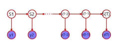
Figure 1. HMM Graphical Model [13]

In order to specifying the priors, we let the observation parameters φ be independent and identically distributed drawn from a prior distribution H. Then the prior for the transition probabilities are symmetric Dirichlet distributed. The simple way to obtain infinite states of iHMM is to use symmetric Dieichlet priors over the transition probabilities with parameter α/K and take K → ∞. This methods has been successfully used to derive DP mixture models[14]. To get to know across transitions, we may use a hierarchical Bayesian formalism.

πk ~ Dirichlet(αβ),

β ~ Dirichlet(γ/K…γ/K)

(1)

where

πkare transition probabilities and β are the prior parameters.

A HDP is a set of Dirichlet processes (DPs) connected through a shared random base measure which is itself drawn from a DP [16]. Generally, each

Gk∼ DP (α,

G0) with shared base measure

G0can be understood as the mean of

Gk, and concentration parameter α > 0, which governs variability around

G0. The shared base measure is itself given a DP prior:

G0 ~ DP(γ, H)with H a global base measure. Then random measures are expressed as

G0= ∑k’∞βk’δφk’, and

Gk= ∑k’=1∞πkk’δφk’, where

β ~ GEM (γ)is the stick-breaking construction for DPs,

πk ~ DP(αβ), and each

φk’ ~ Hindependently. Then we can define the iHMM as follows:

β ~ GEMγ, πk|β~DPα,β, φk ~ H,  (2)

stst-1~Multinomialπst-1, yt| st~F(φst)  (3)

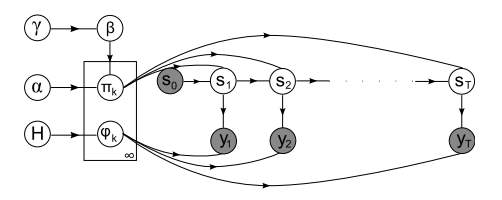
Figure 2. iHMM Graphical Model [13]

The graphical model of iHMM model is shown in figure 2. Thus

βkis the prior mean for transition probabilities leading into state

k’, and α governs the variability around the prior mean. If we fix β = (1/ K . . . 1/K, 0, 0 . . .) where the first K entries are 1/K and the remaining are 0, then transition probabilities into state

k’will be non-zero only if

k’∈ {1 . . .K}, and we recover the Bayesian HMM of [17].

Finally we place priors over the hyperparameters α and γ. A common solution, when we do not have strong beliefs about the hyperparameters, is to use gamma hyperpriors: α ∼ Gamma (

aα,

bα) and γ ∼ Gamma (

aγ,

bγ). [6] describe how these hyperparameters can be sampled efficiently, and we will use this in the experiments to follow.

2. Application of iHMM

Infinite Hidden Markov models can be used in many different areas for modeling the structure of data. In Fine’s paper [18], he and his coworkers introduce several widely used hidden applications, such as language and speech processing, information extraction, video structure discovery and activity detection and recognition.

In Matther’s paper [9], their proposed to clustering gene expression time course data treat the different time points as independent dimensions and are invariant to permutations. They describe the iHMM in the framework of the HDP, in which an auxiliary variable Gibbs sampling scheme is feasible. They also show for two-time course gene expression data sets that HDP-HMM performs similar and better than the best finite HMMs found by model selection.

1.      Identifying speculative Bubbles

In Shu-Ping Shi and Yong Song’s paper [19], they proposed a method to use iHMM to detect and evaluate speculative bubbles. In their opinion, their chose iHMM due to the three benefits: 1) the iHMM has high capable with capturing the nonlinear dynamics of a variety of bubbles outcomes since iHMM allows an infinite number of states; 2) In a coherent Bayesian framework, their implementation to detection, dating and estimating of bubbles are straightforward; 3) to use iHMM to assume hierarchical structures is surpassing in out-of-sample prediction. Shu-Ping and Yong discussed two empirical applications in their work, the first one is Argentina money base, exchange rate and consumer price from Jan. 1983 to Nov. 1989. The second is U.S. oil price from Apr. 1983 to Dec. 2010. In their result and model comparison, they found that the iHMM is persuasively supported by the predictive likelihood.

Bubbles are germs of economic and financial instability which attracts many economists and data analysts over years. However, there still no general agreement on how those bubbles been generated. There are two perspective among bubbles’ explosive, Evans[20] recommends there is a periodically collapsing explosive process for bubbles when it is over a certain threshold and the expands rate is faster when bubbles survives. On the other hand, Phillips et al. [21] presented a local explosive process and they think bubbles behavior is a temporary phenomenon. In other words, when bubbles slide back to the level before origination upon collapsing, the asset process transfer from a unit root regime to an explosive regime. Overall, although both aforementioned processes have been proposed as data generating process frequently but there still do not have been justified by any data series includes bubble episodes.

1.       Empirical Application: Argentina Hyperinflation

As mentioned in last section, the first application that proposed in Shu-Ping’s paper is to apply iHMM to the money base, exchange rate and consumer price in Argentina from Jan. 1983 to Nov. 1989. The money base is a proxy for market fundamental and the exchange rate data series is to determine bubble-like behavior. In this application, the aim is to examine whether there are bubble behaviors in the consumer price.

As a standard, author estimate a two-regime Markov-switching (MS2) model [22] using the Bayesian approach, which is

∇yt| st=j, Y1,t-1~ N (ϕj0+ βjyt-1+ϕj1 ∇yt-1+…+ϕj4 ∇yt-4, σj2)

Pr ⁡st=j, st-1=j= pjj

with j = 1,2. Figure 3 shows the posterior probabilities of

βst>0for the logarithmic money base (1^st plot), exchange rate (2^nd plot) and consumer price (3^rd plot). The dotted line represents MS2 model illustrates that when posterior probability exceeds the 0.5 in June 1985 and July 1989 for the three test data series, suggests the existence of explosive behaviors. Nevertheless, there is also bubbles in the exchange rate emerge in Apr. 1987, Oct. 1987 and Sept. 1988 which have some locally explosive dynamics which can not be explained by the money base. Besides the posterior probabilities, they also provide and display the posterior mean of

βstin order to support their measurement, which can be found in [22]. In figure 3, dashed line represents the posterior probability with using iHMM model. It shows similar outcomes of money base to those from the MS2 model. Hence, it is reasonable to have a two-regime specification for the money base. However, for the exchange rate and consumer price, the iHMM shows distinct measurement. As for the exchange rate, any plunge of the iHMM is associated with a decrease of the exchange rate, while for the MS2 model, there are 4 spikes correspond to a decrease of the exchange. The reason that author come up with is due to the limited number of regimes in the MS model. There are 3 regimes in iHMM based on figure 3: first at July 1989 which is associated with bubble emerging; second causing the exchange rate decrease which is June 1985, April 1987, Oct. 1987 and Sept. 1988; the last one is for the rest of sample. However, the MS2 model combines the first two regimes into one which results in confusing outputs. For the consumer price, iHMM model shows there are bubbles through the whole period. Although the MS2 model found two bubble periods at Jun 1985 and July 1989, the MS2 still cannot capture the dynamics due to the limited number of regimes.

Figure 3. The growth rate and the posterior probabilities of

βst>0 the money base, exchange rate and consumer price

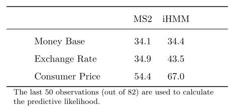
Finally, Shu-Ping concludes that the dynamic pattern of the money base are similar to locally explosive of Peter [21]. On the other hand, the dynamics of the exchange rate and the consumer price are likely to the periodically collapsing behavior of Evans [20]. Shu-Ping also proposed a log predictive likelihoods table in Table 1 shows that the predictive likelihood of money base is close which is same with figure 3. The exchange rate and the consumer price from the iHMM are much higher which further reject the MS2 mode for the exchange rate and the consumer price.

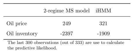
Table 1. Log predictive likelihoods

2.       Empirical Application: U.S Oil Price

The second application introduced in this paper experiment the existence of speculative bubble behaviors in the U.S oil price. In this application, most studies have found evidence of bubble existence. In this paper, the data is sampled from April 1983 to Dec. 2010 and author applied both the MS2 model and the iHMM to the logarithmic real oil price and the logarithmic oil inventory. Similarly, they also proposed the posterior probabilities of

βst> 0and the results are shown in figure 4. As for oil inventory, the MS2 and the iHMM model proposed consistently which there is no evidence of explosive behavior. In this case, regime switching is not a feature of the oil inventory dynamic among the sample period. For the oil price, there are different results from the MS2 model and iHMM model. No evidence of bubble exists by looking at the MS2 model since the posterior probabilities of

βst> 0are always less than 0.5. However, the iHMM indicates that the oil price dynamics includes mild explosive behavior and bubble collapse phases.

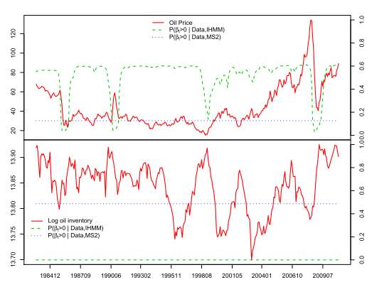
Figure 4. Posterior probabilities of

βst> 0for the logarithmic oil price and inventory

The comparison of the MS2 model and iHMM model for U.S oil price is shown in Table 2. It also presents the log predictive likelihoods as last section. This table reports that iHMM outperforms the two-regime MS model for both data series. The difference for these two models is high which are (321-249) = 72 and (-1909-(-2397)) = 488 which indicates that the iHMM models supports the old price better than the MS2 model.

Table 2. Log predictive likelihoods

2.      Short-term Interest Rates with extension of iHMM models

In finance, models of the term structure of interest rates are important, especial for short-rate. It is usually difficult to model over long periods because of the changes in monetary regimes and economic shocks. In John’s paper [23], they applied the iHMM model and other models to weekly U.S. data and found significant parameter for short-term interest rates change over time.

They applied the iHMM model to the 3-month T-bill of secondary market obtained from the Board of Governors of the Federal Reserve System. It is a weekly, Friday to Friday data from Jan. 15–1954 to Mar-28-2014. There are total 3142 observations in this dataset. The data is shown in figure 5. In this paper, there are extensions of iHMM which applied to the VSK model and the CIR model. Generally, The CIR specification performs the best and the VSK need a few more states on average to fit the data. In empirical application, author focus on x = 1 and 1/2 which stands for the VSK model [24] and CIR model [25], respectively, to the iHMM model with hierarchical prior which corresponding to iHMM-CIR-H and iHMM-VSK-H. More detailed implementation of these two models can be seen in John and Qiao’s paper [23]. Based on their analysis, their new model with hierarchical prior provides a significant improvement in density forecasts. Also, the iHMM-CIR-H also prove to be the best model for density prediction and is better than the best performing benchmark model MS-3-CIR-H [23]. The density forecasts for the iHMM-VSK-H presents a bit less variation. The RMSE for both models is very robust to the change in the prior.

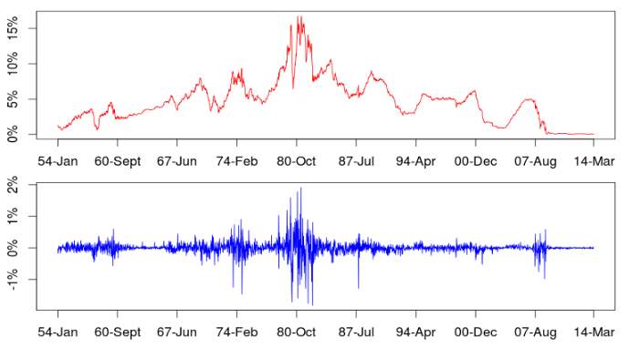
Figure 5. Weekly 3-Month T-bill Rate Level (top) and Change (button)

3.      Infinite Hierarchical Hidden Markov Models (iHHMM) and its application

Hierarchical Hidden Markov Models (HHMM) also useful statistical model derived from the HMM. Each state of a HHMM model is a self-contained probabilistic model[26]. It has been widely used in many modeling cases for sequential data applications like speech recognition or text information extracting. To extend this model into unbounded number of levels in the hierarchy, Katherine and Yee[11] proposed iHHMM model which is more flexible to model sequential data. It allows a potentially infinite number of levels in the hierarchy but required the specification of a fixed hierarchy depth. In their model, they use Gibbs sampling and a modified forward-backtrack algorithm to perform inference and learning. The graphical model for iHHMM can be seen in figure 6.

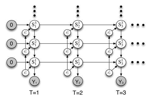
Figure 6. Graphical model for the iHHMM[11]

In their work, they infer characters in written text using their iHHMM model and compared the results with a standard HMM model learned using the EM algorithm and a one level HMM model learned using Gibbs sampling. Figure 7 reports the difference in log predictive likelihood of the next character in the text using the iHHMM model and the other two completed model algorithms. Top histogram is the difference in log predictive likelihood between the iHHMM and HMM learned using EM algorithm, the button is log predictive likelihood between the iHHMM and a one level HMM learned using Gibbs sampling. The long tail specifies that there are letters can be better predicted by learning long range correlations. The top histogram shows a long tail where iHHMM is performing significantly better on some letter than the one level Gibbs HMM. This is because many letters can be predicted with only one level of hierarchy structure while some others can be better predicted by learning long range correlations through iHHMM model. There are more tails in button histogram which indicates that iHHMM performs much better performance than the traditional HMM with EM algorithm.

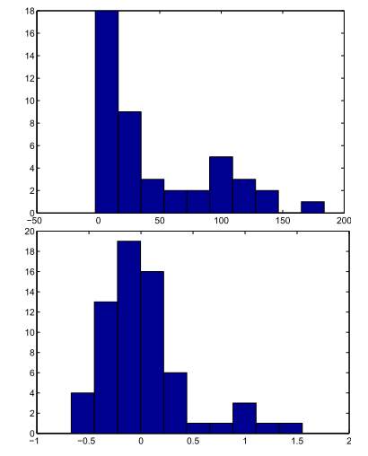
Figure 7. Alice in Wonderland letters data set. Top: The difference in log predictive likelihood between the IHHMM and a standard HMM learned using the EM algorithm. Bottom: The difference in log predictive likelihood between the IHHMM and a one level HMM learned using Gibbs sampling. [11]

3. INFERENCE ALGORITHMS FOR IHMM

Infinite Hidden Markov Models are been one of the attractive nonparametric extension of the widely used hidden Markov model. There are several existing inference algorithms for iHMM modeling. I did some literatures mainly on those approaches for iHMM such as Beam sampling and Particle Gibbs sampling algorithms. Several algorithms are discussed and compared in this paper and based on the research in this section. Those algorithms mentioned in this paper demonstrate significant convergence improvements on synthetic and real-world data sets which prove to be competitive methods for iHMM.

1.      Beam sampling

In Jurgen Van Gael and Yunus Saatchi’s paper [13], they proposed application of iHMM inference using the beam sampler on changepoint detection and text prediction problems. Previously, the only approximate inference algorithm available is Gibbs sampling [27] which is a Markov chain Monte Carlo algorithm for obtaining a sequence of observations which are widely used as a means of statistical inference and individual hidden state variables are resampled conditioned on all other variables [6]. The traditional algorithm for iHMM is Gibbs sampler [6]. It is a straightforward implementation but may have some shortcoming. One is that sequential and time series are sometimes to be correlated which is not the ideal situation for the Gibbs sampler. In their paper, Van Gael et al.[13] present beam sampling with combination of slice sampling and dynamic programming to sample the state trajectories efficiently. The basic idea is to apply slice sampling to limit to a finite number of states in each step of the iHMM model and then use dynamic programming to sample whole state trajectories efficiently.

Also, in this paper, Van Gael and his coresearchers evaluate their work compared with Gibbs sampler with two artificial and two real datasets. The two real data are 4050 noisy measurements of nuclear response of rock strata and the “Alice’s Adventures in Wonderland” text data set.

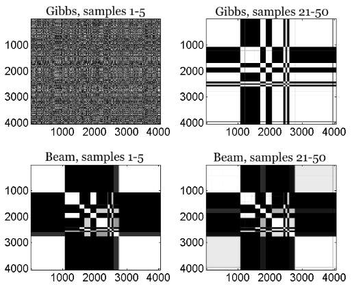
Figure 8. The left plots show how frequently two datapoints were in the same cluster averaged over the first 5 samples. The right plots show how frequently two datapoints were in the same cluster averaged over the last 30 samples

Figure 8 shows the probability that they are in the same cluster over the first five and the last thirty samples using Gibbs sample and beam sample to the nuclear response of rock strata dataset. The plot indicates that the beam sampler mixes faster than the Gibbs sampler and the Gibbs sampler have problem to reassign the state for whole segments while the beam sampler can do it more easily by looking at the right plots. Also, the beam sample is more robust than Gibbs sampler.

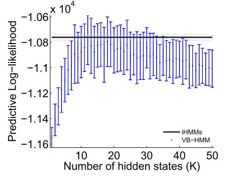
Figure 9. Comparing VB-HMM with the iHMM

Figure 9 presents the log predictive likelihood for the finite HMM using variational Bayes (VB-HMM) and the two iHMM model learned using beam and Gibbs sampling to “Alice’s Adventures in Wonderland” text data set. The iHMM shows significant predictive power when compared with VB-HMM. In this case, iHMM with beam sampling and Gibbs sampling didn’t perfrom much difference and this experiment mainly shows the difference with the use infinite capacity.

4. Particle Gibbs sampling for iHMM

Another sampling method proposed by Nilesh Tripuraneni and his coworkers [16] is Particle Gibbs sampling. In their paper, they present a novel infinite-state Particle Gibbs (PG) algorithm to re-sample state trajectories for the iHMM. This approach uses an efficient proposal optimized for iHMMs and leverages ancestor sampling to improve the mixing of the standard PG algorithm. Detailed implementation of PG algorithm can be found in their paper[16], and the concept that proposed to describe their infinite-state particle Gibbs algorithm for the iHMM can be shown in figure 10.

Figure 10. Steps of implementing infinite-state particle Gibbs algorithm for the iHMM

In their paper, Nilesh conduct experiments on both synthetic data and real dataset. As for synthetic dataset, he compared the performance of the PG sampler, beam sampler and Gibbs sampler on inferring data. The results are shown in figure 11. It applied PG sampler to both the iHMM(PGAS) and the sticky iHMM (PGAS-S). The figure shows that PG sampler converges faster than both the beam sampler and Gibbs sampler.

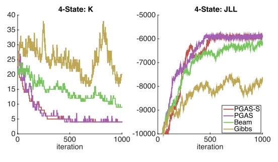
Figure 11. Comparing the performance of the PG sampler, PG sampler on sticky iHMM, beam sampler and Gibbs sampler. Left: Number of “Active” States K vs. Iterations. Right: Joint-Log Likelihood vs. Interations

Nilesh did the similar comparison to “Alice’s Adventures in Wonderland” data, the performance results can be seen in figure 12. By looking at the joint log likelihood, both beam sampler and PG sampler are quickly converging, but the beam sampler in this experiment is learning a transition matrix with unnecessary “active” states. In their results, the time complexity of PG sampler is O(TNK) for a single pass, while the beam sampler has O(T

K2) as its time complexity. Hence, the PG sampler has more competitive to beam sampler.

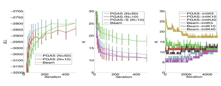
Figure 12. Left: Comparing the Joint Log likelihood vs. Iterations for the PG sampler and Beam sampler. Middle: Comparing the converges of the “active” number of states for the iHMM and sticky iHMM for the PG sampler and Beam sampler. Right: Trace plots of the number of states for different initializations for K

 

5. CONCLUSIONS AND DISCUSSION

It is good to learn about infinity Hidden Markov Models. In this paper, the background of a simple Markov model was introduced at the beginning and we learned that nonparametric Bayesian models caught a lot attention in recent years in machine learning and statistical areas. First, we talks about the Dirichlet process which was first proposed by [6]. Then we discussed several applications and extensions of iHMM. It shows that iHMM model has more flexible and robust to model the sequential data. Then also several inference approaches were discussed in this paper and we found that in Nilesh [16] paper, their methods to use PG algorithms to sampling in iHMM present to be the best performance to data among other samplers such as beam sampler and Gibbs sampler.

REFERENCES

[1] “Markov model – wiki.” [Online]. Available: https://en.wikipedia.org/wiki/Markov_model.

[2] Wiki, “Hidden Markov Model.” [Online]. Available: https://en.wikipedia.org/wiki/Hidden_Markov_model.

[3] T. Baum, L.E.Petrie, “Statistical Inference for Probabilistic functions of Dinite State Markov Chains,” no. Ann. Math. Stat., p. 1554–156., 1996.

[4] T. Baum, L.E.Petrie, “A Maximization technique occurring in the statistical analysis of probabilistic functions of markov chains,” Ann. Math. Stat., vol. 41, pp. 164–171, 1970.

[5] L. R. Rabiner, “A tutorial on hidden Markov models and selected applications in speech recognition.,” Proc. IEEE, vol. 77, 1989.

[6] Y. W. Teh, M. I. Jordan, M. J. Beal, and D. M. Blei, “Hierarchical Dirichlet Processes,” pp. 1–30, 2005.

[7] L. Baum., “An Inequality and Associated Maximization Technique in Statistical Estimation for Probabilistic Functions of Markov Processes,” Inequalities III Proc. Third Symp. Inequalities, pp. 1–8, 1972.

[8] J. M. Maheu and Q. Yang, “An Infinite Hidden Markov Model for Short-term Interest Rates,” J. Empir. Financ., vol. 38, no. January, pp. 1–33, 2015.

[9] M. J. Beal, “Gene Expression Time Course Clustering with Countably Infinite Hidden Markov Models,” 2005.

[10] C. Guo and Y. Zou, “Multi-granularity Video Unusual Event Detection Based,” pp. 264–272, 2011.

[11] K. A. Heller, “Infinite Hierarchical Hidden Markov Models,” vol. 5, pp. 224–231, 2009.

[12] M. Gales and S. Young, “The Application of Hidden Markov Models in Speech Recognition,” vol. 1, no. 3, pp. 195–304, 2008.

[13] J. Van Gael, “Beam sampling for the infinite hidden Markov model Beam Sampling for the Infinite Hidden Markov Model,” no. May, 2014.

[14] C. E. Rasmussen, “The Infinite Gaussian Mixture Model,” pp. 554–560, 2000.

[15] M. J. Beal and C. E. Rasmussen, “The Infinite Hidden Markov Model.”

[16] N. Tripuraneni, “Particle Gibbs for Infinite Hidden Markov Models,” Adv. Neural Inf. Process. Syst., pp. 2386–2394, 2015.

[17] D. J. C. Mackay, “Ensemble Learning for Hidden Markov Models,” no. 1995.

[18] F. Park, “The Hierarchical Hidden Markov Model : Analysis and Applications,” vol. 62, pp. 41–62, 1998.

[19] S. Shi, “Identifying Speculative Bubbles with an Infinite Hidden Markov Model,” 2011.

[20] G. W. Evans., “Pitfalls in testing for explosive bubbles in asset prices.,” Am. Econ. Rev. 81(4)9, vol. 22, p. 930, 1991.

[21] P. C. B. Phillips, Y. Wu, and J. Yu, “Explosive behavior in the 1990s Nasdaq: When did exuberance escalate asset values?,” Int. Econ. Rev. (Philadelphia)., vol. 52, pp. 201–226, 2011.

[22] S.-P. Shi, “Bubbles or volatility: A markov-switching adf test with regime-varying error variance.,” 2010.

[23] J. M. Maheu and Q. Yang, “An Infinite Hidden Markov Model for Short-term Interest Rates,” Munich Pers. RePrc Arch., no. 62408, 2015.

[24] O. Vasicek, “An equilibrium characterization of the term structure,” J. financ. econ., vol. 5, pp. 177–188, 1977.

[25] J. Cox, J. Ingersoll, and R. Ross, “A theory of the term structure of interest rates,” Econometrica, vol. 53, pp. 385–407, 1985.

[26] Wiki, “Hierarchical Hidden Markov Models.” [Online]. Available: https://en.wikipedia.org/wiki/Hierarchical_hidden_Markov_model.

[27] wiki, “Gibbs sampler.” [Online]. Available: https://en.wikipedia.org/wiki/Gibbs_sampling.