Dissertation on Predicting Greenhouse Gas Emissions of Vehicles

APPLICATION OF ADAPTIVE NEURO-FUZZY TECHNIQUE FOR PROJECTION OF GREENHOUSE GAS EMISSIONS FOR ROAD SECTOR

Abstract

Numerous studies have been conceded worldwide to predict greenhouse gas (GHG) emissions using different methods. Most of the methods are not capable enough to provide good forecasting performances due to the problems of non-linear data. Adaptive Neuro-fuzzy inference system (ANFIS) is one of the well-known methods with its ability to deal with nonlinear problems. However, the performance of this model in predicting GHG emissions is not immediately known. This paper presents the performance of the fuzzy-based model in the prediction of GHG emissions in the USA. The model inputs were simulated using USA data for the period from 1990 to 2012. The ANFIS model was developed using the ratio between Vehicle-kilometres and Number of Transportation Vehicles for six transportation mode such as Light Trucks, Single-unit trucks, Tractor and Bus.The prediction performance was measured using root means square error.

Keywords: Modelling, neuro-fuzzy, greenhouse gas emissions, Fuzzy inference systems.

Introduction

Air pollution is one of the major environmental issues involved worldwide. This environmental problem is mainly due to the high concentrations of greenhouse gases (GHGs) such as carbon dioxide (CO2) and other gases in the atmosphere.

Since the introduction of motorized transportation systems, economic growth and advancing technology have allowed people and goods to travel farther and faster, steadily expanding the utilization of energy for transportation. Current transportation systems are overwhelmingly powered by internal combustion engines fueled by petroleum. Emissions of greenhouse gas (GHG) produced by the transportation sector, have regularly increased along with travel, energy use, and oil imports. In the lack of any constriction or active countermeasures, transportation energy use and GHG emissions will continue to increase (Greene & Plotkin 2003).

Increasing motorization across the world has caused a stable increase in GHG emissions in the transport sector, which accounted for about 23% of total worldwide GHG emissions in 2007, of which approximately 73% have been produced by road transport (Association 2008).

All over the world, people become more aware of the impact of greenhouse gases on the environment. During the last decades, individuals, organizations and governments have come to realise that the emission of greenhouse gases needs to be reduced (Loo 2009).

Several studies have been conducted to predict GHG emissions in order to overcome their impact on the environment. However, many researchers face difficulties in predicting GHG emissions because they involve non-linear relationships and uncertainty of variables. Emissions from certain natural and human sources, for example, forest fires, industry, road and air traffic are often uncertain and not usually available. On the other hand, it is known that official emission data cannot be considered as entirely reliable (Pokrovsky, Kwok & Ng 2002). It is therefore necessary to have a reliable way to predict GHG emissions due to uncertainty and non-linear data. Accurate and robust prediction of GHG emissions would be too great to overcome the environmental problems.

Environmental data is usually very complex to model due to the underlying correlation between several variables of a different type that results in complex network relationships. The development of tools for predicting GHG emissions has attracted the attention of many scientists. Predictions are based on information including past historical data. Apart from that, there are many ways that have been applied in predicting GHG emissions. From the literature review, most of the methods to predict GHG emissions are aimed to increase the accuracy of the results (Pauzi & Abdullah 2014).

A few researchers (Jain & Khare 2010; Morabito & Versaci 2003) have succeeded in applying ANFIS to model and forecasting CO2 emissions in various fields. However, it has been seen from the literature that there are not many studies using this method to predict GHG emissions.

The aim of this paper is to examine the transport related factors for greenhouse gas emissions through adaptive neuro-fuzzy technique. This will enable to calculate the GHG generated from the road sector and will be a valuable resource for the planners to adopt appropriate measures towards optimizing the travel demand.

The remainder of the paper is organized as follows. In next section we present literature review which is followed by the research methodology. Results obtained from adaptive neuro-fuzzy technique to predict and forecast the greenhouse gas emission are presented next. The final section presents the conclusions and recommendations for future research.

Literature Review

A review on the literature has shown that emission factors in transport have been mentioned in many researches in many countries of the world. These factors are heavily affected by transport routes, the size and age of the vehicles deployed (Binh & Tuan 2016).

Current research literature on the transport sector’s CO2 emissions is mainly divided into four categories and from a methodological perspective. The first category is the bottom- up sector based analysis. Using the method of bottom-up analysis,(van der Zwaan, Keppo & Johnsson 2013) explores CO2 emissions of European transport sector and how it can be decarbonized, and (Bellasio et al. 2007) develop the COPERT III methodology to analyse the emissions from road traffic in Italy. The method is also used in the study of vehicle emissions in city areas (Dallmann et al. 2013; He & Chen 2013; Sider et al. 2013).

The second method is the index decomposition analysis. The transport sector’s CO2 emissions are generally decomposed into changes in fuel mix, modal shift, economic growth, population, emission coefficients and transport energy intensity. Specifically, (Timilsina & Shrestha 2009) show that economic growth and transport energy intensity are the principal factors in Latin American and Caribbean (LAC) and Asian countries and decayed CO2 outflows development into sections associated with changes in modal shift, emission coefficient, fuel mix and transportation energy intensity along with GDP growth. (Chandran & Tang 2013) and (Andreoni & Galmarini 2012) come to a similar conclusion that economic growth play a greater role in contributing to CO2 emissions in EU27 and ASEAN-5 economies. (Lakshmanan & Han 1997) credited the change in transport segment CO2 discharges to the development in GDP, DT and populace.

The third method is system optimization. This method has been widely used in forecasting energy demand and CO2 emission (Ahanchian & Biona 2014; Motasemi et al. 2014; Si et al. 2012); in analysing integrated energy planning for sustainable development (Szendrő & Török 2014); and in designing energy supply networks (Kanzian et al. 2013). There is a number of optimisation models were created to maintainable vitality arranging and CO2 emanation diminishment. Utilizing linear programming models, (Bai & Wei 1996; Börjesson & Ahlgren 2012; Wang, C et al. 2008)  explored the cost effectiveness of conceivable CO2 reduction choices for the energy industries. Furthermore, utilizing a mixed integer linear programming model, (Hashim et al. 2005) contemplated the impacts of fuel balancing and fuel switching choices on power generation. Their studies discovered that FE and fuel switching are the best choice to decrease CO2 discharges. (Tan et al. 2013) utilized mixed integer linear programming analysis for the perfect arranging of waste to vitality that minimizes electricity generation costs and CO2 emissions.

The fourth method is econometric models. Using time series econometric models, (Saboori, Sapri & bin Baba 2014) investigates long run nexus between economic growth and the transport sector’s CO2 emission in OECD countries. (Lu, Lewis & Lin 2009) predict the development trends of motor vehicle population, vehicular energy consumption and CO2 emission in Taiwan. (Tolón-Becerra et al. 2012) examine the distributed dynamic CO2 emission reduction targets for EU countries. (Meyer, Leimbach & Jaeger 2007) estimate passenger car demand and associated CO2 emission in 11 world regions. (Tokunaga & Konan 2014) and (Konur 2014) use panel data to estimate CO2 emissions in the transport sector. (Sultan 2010) found co-combination of pay per capita and fuel price (FP) on transport fuel consumption (FC), while (Ang 2008; Bekhet, H & Yasmin 2013; Bekhet, HA & Yusop 2009; Ediger & Akar 2007; Wang, SS et al. 2011) discovered a relationship between vitality utilization and CO2 discharges. (Begum et al. 2015) considered the impact of GDP, FC and populace development on the CO2 emissions. (Ivy-Yap & Bekhet 2015) study recommended that the FC and CO2 emission development could be reduced by using low-carbon advancements. Utilizing regression analysis, (Sadorsky 2014) explored the relationship between vitality force, urbanization, salary and GDP and found that diminishment in CO2 emissions could grow from increases in FE and fuel changing from fossil fuels to renewables vitality. (Shu & Lam 2011) found that the CO2 emissions were absorbed around the thick road network of urban territories with high populace density. (Alhindawi et al. 2016) identified the main drivers of greenhouse gas emission for road sector using ratio between Vehicle-kilometres and Number of Transportation Vehicles for six transportation modes.  (Xu, He & Long 2014) found the effects of populace, vitality structure, GDP and vitality intensity on CO2 emanations. Their study discovered that the driving components of CO2 emanations were the GDP took after by the populace scale and vitality structure.

Most of the researcher used the time series analysis to predict the GHG emissions. Furthermore, there are few studies that used adaptive neuro-fuzzy technique to predict and forecast the greenhouse gas emission. (Jang, JSR 1993; Shi & Mizumoto 2000) and (Jang, JSR & Chuen-Tsai 1995) list the applications of neuro-fuzzy approach, also describing the theoretical basis of the model.

The neuro-fuzzy technology combines ANN and fuzzy logic. It effectively integrates the learning ability of neural networks into the development of a fuzzy inference system. That is, it helps to determine the membership functions and fuzzy rules by learning from data using a neural network. In this way, the accuracy of modeling by the fuzzy system can be greatly enhanced. Because of the different connections between ANN and the fuzzy system, a number of neuro-fuzzy models can be found in the literature (Horikawa, Furuhashi & Uchikawa 1992; Khajeh, Modarress & Rezaee 2009). The adaptive-network-based fuzzy inference system (ANFIS) discussed by (Jang, JSR 1993; Jang, JSR & Chuen-Tsai 1995) was a Sugeno type fuzzy inference system implemented within an adaptive neural network with the ability to learn under supervision. It has been successfully applied in fields such as automatic control, data classification, decision analysis, expert systems, and computer vision. Because of its multi-disciplinary nature, and all have achieved high accuracies (YEH, TSAY & LIANG 2005; Zhou, Chan & Tontiwachwuthikul 2010).

Methodology

Several models have been previously proposed to model and forecast the greenhouse gas emissions, ranging from relatively simple ones, such as that proposed by (Choi, Roberts & Lee 2014) which consists of only a single model for forecast the CO2 emissions from the transportation sector, to more complex models, such as that developed by (Begum et al. 2015) which consists of several modules that interact with each other through an integration module.

This study will use the analysis of neuro-fuzzy technique to identify the most important variables that affect the greenhouse gas emissions for road sector.

ANFIS is an architecture which is functionally equivalent to a Sugeno-type fuzzy rule base. This learning algorithm uses a set of training data to adjust the base of the current rule in order to adapt to neuro-fuzzy. Training data are used to teach the neuro-fuzzy system by adapting its parameters and using a standard neural network algorithm which utilizes a gradient search, so that the mean square output error is minimized (Al-Ghandoor & Samhouri 2009).

Variables

In the open literature, previous research papers have taken into consideration variables such as fuel price (FP), fuel consumption (FC), gross domestic product (GDP) and road density. This study utilizes advantages of such experience and introduces other new important variables such as the ration between Vehicle-kilometres travelled (VKT) and Number of Transportation Vehicles (NTV) for six transportation mode. These variables are briefly explained in the following section, along with reasons for their inclusion in the current proposed model.

Vehicle-kilometres travelled (VKT)

The motor vehicle fleet is characterised in terms of vehicle activity levels or traffic volume, expressed as vehicle kilometres travelled (VKT). Estimates of VKT are used extensively in transport planning for allocating resources, estimating vehicle emissions, computing energy consumption and assessing traffic impact. In addition, VKT estimates can also contribute information necessary to inform infrastructure investment decisions and road safety policy. Therefore, it is critical to have an accurate estimation of VKT (Bureau of Infrastructure 2011).

Number of Transportation Vehicles (NTV)

The new categories of vehicle include passenger car, light trucks (“other 2-axle, 4-tire vehicles”), “single-unit 2-axle 6-tire or more truck” and combination truck tractors. The greenhouse gas emissions may increase due to the increased on Number of Transportation Vehicles.

Data Sources

The historical data on Vehicle-kilometres by Mode (VKM) and Number of Transportation Vehicle (NTV) of road transport from the year 1990 to year 2012 for the current study was collected from official data sources. These data are utilized to develop different models that are based on neuro-fuzzy analyses. The source of information for data was the North American Transportation Statistics (NATS) online database (North American Transportation Statistics 2000).

Data Limitations

NTV Road data are based on statistics compiled by the Federal Highway Administration (FHWA) at the U.S. Department of Transportation from reports submitted by the states. In 1995, FHWA revised the data series for the number of U.S. road vehicles. The new categories include passenger car, light trucks (“other 2-axle, 4-tire vehicles”), “single-unit 2-axle 6-tire or more truck” and combination truck tractors. Pre-1993 data were assigned to the closest available category. Data for light trucks or “other 2-axle, 4-tire vehicles” include vans, pick-up trucks and sport utility vehicles. “Single-unit 2-axle 6-tire or more trucks” are on a single frame with at least two axles and six tires, and correspond to the category of single-unit trucks. Combination truck tractors correspond to the category of tractors. Passenger cars include taxis. The total for buses is based on FHWA estimates and includes intercity, charter, school and local motor bus. The estimate of local motor buses is based on data from the American Public Transit Association (APTA). All road data represent registered vehicles in the U.S., except local motor buses that are active passenger vehicles. VKM Road data include passenger cars, motorcycles and light trucks. In January 1997, the FHWA published revised vehicle-kilometres data for the highway mode for several years. The major change reflected the reassignment of some vehicles from the passenger car category to the light truck category (North American Transportation Statistics 2000).

Therefore, we acknowledge that the discontinuities within the time-series data as stated above may introduce some errors to our model’s estimation. However, the generality of the method proposed and the results obtained in this study could be tested further in future once a good and detailed data set is available.

Adaptive Neuro-Fuzzy Model (ANFIS)

ANFIS has proved to be an excellent function approximation tool (Jang, JSR 1993; Takagi & Sugeno 1985). The MATLAB ANFIS algorithm provides a method for the fuzzy modelling to learn information about a data set, in order to compute the membership function parameters that best allow the associated fuzzy inference system to track the given input-output data (Jang, JR 1997). This learning method works similarly to that of neural networks ANN.

A weakness of the ANN approach is that it does not explain the nature of relationships between the parameters of the process, and the neuro-fuzzy modelling approach has been applied to address this weakness. The ANFIS model is used to develop fuzzy inference systems which interpret the interrelations between the parameters by learning from the dataset of historical data (Zhou et al. 2011).

Learning Algorithm and Architecture of ANFIS

An ANFIS consists of nodes connected through the directional links, and each node performs a specific function on the incoming signal. Some nodes adapt and contain a set of parameters. The output of the adaptive nodes depends on these parameters, whose values can be changed during the learning process based on the given training data so as to reduce a prescribed error measure (Jang, JSR 1993; Jang, JSR & Chuen-Tsai 1995; YEH, TSAY & LIANG 2005).The hybrid learning algorithm, combining the back-propagation gradient descent method and the least squares estimate (LSE), is used as learning rules of the adaptive networks (Zhou et al. 2011).

From the ANFIS architecture, shown in Figure 1, it is observed that for given values of premise parameters, the overall output can be expressed as a linear combination of the consequent parameters (Jang, JSR 1993).

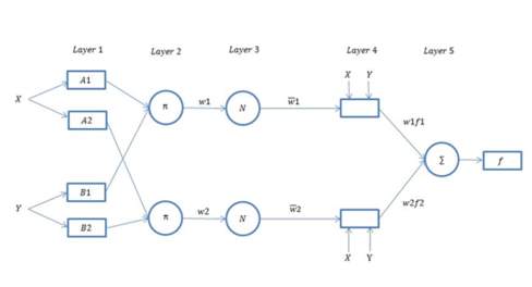
Figure 1 ANFIS Architecture

The functions of each layer are summarized as follows(Bektas Ekici & Aksoy 2011):

Layer 1: The outputs of the nodes of this layer are the membership values due to input samples and used membership functions. To simplify the structure

xand

yare assumed to be the input nodes,

Aand

Bare the linguistic labels,

μAiand

µBiare the membership functions outputs obtained from these nodes are expressed below.

Oi=1µAix

i=1,2

for

2

Oi+2=1µBix            i=3,4

The membership functions

µAiand

µBiare usually assumed to be bell-shaped with maximum equal to1 and minimum equal to 0. While

miis the middle point of bell-shaped membership function and

σ1is the standard deviation

µ(x)can be calculated as given in Eq. (3);

µx= 11+x-ciai2bi                                                                    3

where

ai,

bi, and

ciare the premise parameters.

Layer 2: In this layer, the firing strength of each rule is calculated by mathematical multiplication.

Oi2= wi=  μAix. µBiy    for      i=1,2                                4

Layer 3: In this layer, the normalization of the firing strengths is performed. The ith node calculates the ratio of the ith rule’s firing strength to all rules firing strength.

Oi3= wi¯= wiw1+w2       for      i=1,2                                       5

Layer 4: The output of each node in this layer is simply the product of the normalized firing strength and a first-order polynomial. Where

f1and

f2are the fuzzy if-then rules as follows the outputs written as given in Eq. (6)

Rule 1: if

xis

A1and

yis

B1then

f1=

p1x + q1y + r1

Rule 2: if

xis

A2and

yis

B2then

f2=

p2x + q2y + r2

Oi4= w¯ifi= w¯ipix+ qiy+ ri                                                 6

where linear

p,

qand

rare the parameters referred to as the consequent parameters.

Layer 5: This node computes the overall output of ANFIS as the summation of all incoming signals from the 4th layer.

Oi5= ∑iw¯ifi = ∑iwi fi∑iwi                                                                7

The final output of adaptive neuro-fuzzy inference system is expressed as:

fout= w¯1f1+ w¯2f2= w1w1+ w2 f1+ w2w1+ w2 f2= w¯1xp1+ w¯1yq1+ w¯1r1+w¯2xp2 + w¯2yq2+ w¯2r2                                                                     8

Division of the data

The Dataset was used to develop different models using the neuro-fuzzy analysis. Each set of data is obtained by randomly dividing the entire data into three subsets for neuro-fuzzy modeling: (1) a training dataset for training the ANFIS to learn about the input-output mappings, (2) a checking dataset used together with the training dataset in the learning process to prevent model overfitting, and (3) a testing dataset used to validate the model to verify the generalization capability of the developed fuzzy inference system (Zhou et al. 2011).

Developing the ANFIS Model

The first step in the development of the fuzzy inference system involves determining the types and number of membership functions for the input and output variables for ANFIS in order to create the fuzzy inference system.

Take for example the parameter of passenger cars (PC); its operating range can be divided into three regions, which can be linguistically described as “high”, “medium”, “low”, according to the experienced operators. Therefore, the initialized membership function of PC includes three subsets, which are respectively defined by the three linguistic variables. The details of membership functions of all six input variables for modelling GHG emissions are listed in Table 1. The Gaussian function was selected to be the form of the membership function, and the centre and width of each membership function were initialized by ANFIS. These parameters associated with the membership functions will be adjusted during the training process.

ANFIS modelling and prediction of greenhouse gas emissions start by obtaining a data set (input-output data points), and dividing it into training and validating data sets. The training data set is used to find the initial premise parameters for the membership functions by a model with an actual system for validating purposes. Figure 2 shows the ANFIS training and modelling process.

Table 1 Input Membership Functions for Greenhouse Gas Emissions

Input Parameters	Number of MF	Linguistic Variables
Passenger Cars (PC)	3	High, Medium, Low
Motorcycles (M)	3	High, Medium, Low
Light Truck (LT)	3	High, Medium, Low
Bus (B)	3	High, Medium, Low
Single Unit Trucks (SUT)	3	High, Medium, Low
Tractors (T)	3	High, Medium, Low

 

 

Fuzzy rules

Fuzzy rules have been developed using MATLAB 7.0, Sugeno type FIS (Sugeno & Kang 1988; Takagi & Sugeno 1985). The total number of all possible fuzzy rules with N number of inputs is determined as,

Number of fuzzy rules =

MN×T                                                                      1

Where N is the number of model inputs, M, the number of fuzzy MFs representing each input, and T, the number of fuzzy MF representing the model output.

Take for example the parameter of GHG emissions, since the numbers of membership functions associated with the six input variables are all three, our 6-dimensional input space can be partitioned into

36= 729 subspaces, which determines that the fuzzy inference system for GHG emissions will contain 729 rules based on the algorithm of grid partitioning.

 

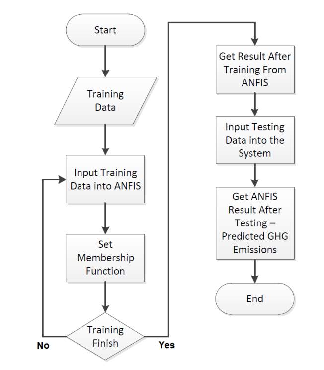
FIGURE 2 ANFIS Flowchart

Results and Discussions

Adaptive Neuro-Fuzzy Analysis

The fuzzy logic toolbox of Matlab 7 was used to obtain deemed results. A total of 1503 nodes and 729 fuzzy rules were used to build the fuzzy systems for modelling and forecasting the greenhouse gas emissions for the road sector.

ANFIS Prediction of Greenhouse Gas Emissions

In our study, a fuzzy inference system was developed after the training process was completed, i.e., the membership functions of the input variables were adjusted and the rules were generated. The structure of a sample inference system for greenhouse gas emissions is shown in Figure 6.

The six input variables all contain three Gaussian membership functions, as shown in the yellow brackets. Although the membership functions of the input variables were initialized by the ANFIS, the training process changed the parameters of the initial membership functions to optimize their representation of the input and output mappings.

Different types of membership functions (MF) of the inputs and output were tested to train the ANFIS prediction system. A three Gaussian-type MF for each input resulted in highly accurate modelling results and minimum training and validation errors. This analysis shows that all the variables have the same effect on the model and there is no variable more important than the others.

The final (MF) were tuned and updated by the ANFIS model to achieve a good mapping of the input variables to the greenhouse gas emissions output. Figure 6 shows the final fuzzy inference system (FIS) used to predict the greenhouse gas emissions.

 

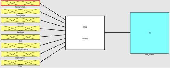
FIGURE 6 Final fuzzy inference systems (FIS) for predicting GHG emissions

The datasets used to build a model that is based on a neuro-fuzzy analysis. Following is the results of the model.

The rule base consists of 729 Sugeno-type rules. The premise part of each rule is a conjunction of linguistic labels of the input variables connected by “AND”; the consequent part is a linear function between the output variable and all the input variables. Assume the six coefficients for the six inputs are

αi,

βi,

δi,

γi,

ρi,

λi, and the constant is

εi, then the ith rule is in the form of:

If Passenger Cars (

PC) is

Al, and Motorcycles (

M) is

Bl, and Light Truck (

LT) is

Cl, and Bus (

B) is

Dl, and Single Unit Trucks (

SUT) is

El, and Tractors (

T) is

Fl, then

Oi

=

αi× (

PC) +

βi× (

M) +

δi× (

LT) +

γi× (

B) +

ρi× (

SUT) +

λi× (

T) +

εi                  (

i=

1,2,…..)

Where

Al, Bl, Cl, Dl, El, Fl,the linguistic labels of membership are functions for each input variable and

Oiare the output in the ith rule.

Since there are 729 rules in the fuzzy inference system for GHG emissions, there will be 729 output values which are calculated using the 729 linear functions. The final output value is then calculated based on the output value and firing strength of each rule.

The neural network training for building a fuzzy model for predicting the greenhouse gas emissions used 19 training data points and 1000 learning epochs. Figure 3 shows the training curve of ANFIS with root mean square error (RMSE) of 40.38 (i.e., almost 0.002%). A comparison between the actual and ANFIS predicted greenhouse gas emissions values after training is shown in Figure 4, which shows that the system is well-trained to model the actual greenhouse gas emissions. The ANFIS-predicted greenhouse gas emission is shown in Figure 5 as a surface plot of GHG emissions as a function of the ratio Vehicle-kilometres by Mode (VKM) and Number of Transportation Vehicle (NTV) for Personal Vehicle (PC) and Commercial Vehicle (CV)

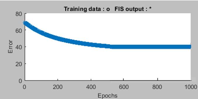
Figure 3 ANFIS training curve

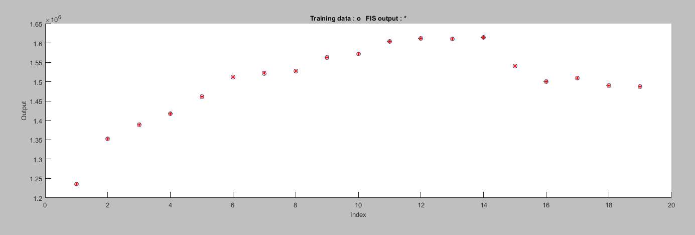
Figure 4 Actual and predicted GHG emissions values

 

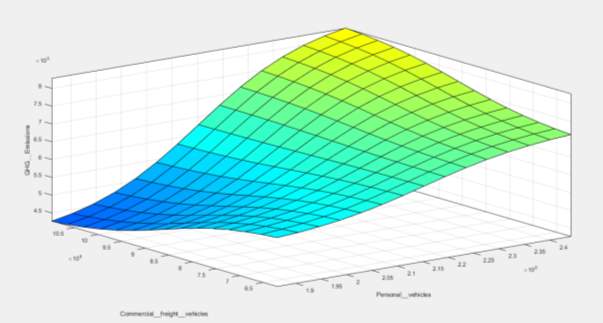
Figure 5 A model for predicting GHG emissions

Conclusions

Air pollution in many developing countries is currently a major concern because of its economic activities. Public awareness of this problem has emerged among its citizens because of the available information on the harmful air pollution to human health and environmental sustainability.

The proposed methods were applied to data from the United States of America, which ranged from 1990 to 2012. Two significant factors were considered.The significant factors affecting greenhouse gas emissions have been found the ratio Vehicle-kilometres by Mode (VKM) and Number of Transportation Vehicle (NTV) for six transportation mode output.

ANFIS analysis shows that all the variables have the same effect on the model and there is no variable more important than the others.This shows the importance of ANFIS model in optimizing the prediction of GHG emissions.

The present study shows that ANFIS is a technique that can be used efficiently to model and predict greenhouse gas emissions. It is believed that this approach can be applied to identify many other parameters in different fields.

In the future, further relationships between the process parameters will be studied and the ANFIS method will be applied to an expanded set of a parameter in an attempt to more fully clarify the relationships between a larger set of parameters for GHG emissions. The membership functions and rules developed using the ANFIS method could also serve as a knowledge base that would become the basis for the improvement studies of the GHG emissions.

Acknowledgements

The authors would like to thank the Australia Government Research Training Program (RTP) scholarship which has enabled us to conduct this research project.

REFERENCES

Ahanchian, M & Biona, JBM 2014, ‘Energy demand, emissions forecasts and mitigation strategies modeled over a medium-range horizon: The case of the land transportation sector in Metro Manila’, Energy Policy, vol. 66, pp. 615-29.

Al-Ghandoor, A & Samhouri, M 2009, ‘Electricity consumption in the industrial sector of Jordan: application of multivariate linear regression and adaptive neuro-fuzzy techniques’, JJMIE, vol. 3, no. 1, pp. 69-76.

Alhindawi, R, Nahleh, Y, Kumar, A & Shiwakoti, N 2016, ‘A multivariate regression model for road sector greenhouse gas emission’, paper presented to ARRB Conference, 27th, 2016, Melbourne, Victoria, Australia.

Andreoni, V & Galmarini, S 2012, ‘European CO2 emission trends: A decomposition analysis for water and aviation transport sectors’, Energy, vol. 45, no. 1, pp. 595-602.

Ang, JB 2008, ‘Economic development, pollutant emissions and energy consumption in Malaysia’, Journal of Policy Modeling, vol. 30, no. 2, pp. 271-8.

Association, JAM 2008, Reducing CO2 emissions in the global road transport sector, Tokyo: Japan Automobile Manufacturers Association, Inc.

Bai, H & Wei, J-H 1996, ‘The CO2 mitigation options for the electric sector. A case study of Taiwan’, Energy Policy, vol. 24, no. 3, pp. 221-8.

Begum, RA, Sohag, K, Abdullah, SMS & Jaafar, M 2015, ‘CO2 emissions, energy consumption, economic and population growth in Malaysia’, Renewable and Sustainable Energy Reviews, vol. 41, pp. 594-601.

Bekhet, H & Yasmin, T 2013, ‘Disclosing the relationship among CO2 emissions, energy consumption, economic growth and bilateral trade between Singapore and Malaysia: An econometric analysis’, World Academy of Science, Engineering and Technology, International Journal of Social, Behavioral, Educational, Economic, Business and Industrial Engineering, vol. 7, no. 9, pp. 2529-34.

Bekhet, HA & Yusop, NYM 2009, ‘Assessing the relationship between oil prices, energy consumption and macroeconomic performance in Malaysia: co-integration and vector error correction model (VECM) approach’, International Business Research, vol. 2, no. 3, p. 152.

Bektas Ekici, B & Aksoy, UT 2011, ‘Prediction of building energy needs in early stage of design by using ANFIS’, Expert Systems with Applications, vol. 38, no. 5, pp. 5352-8.

Bellasio, R, Bianconi, R, Corda, G & Cucca, P 2007, ‘Emission inventory for the road transport sector in Sardinia (Italy)’, Atmospheric Environment, vol. 41, no. 4, pp. 677-91.

Binh, NT & Tuan, VA 2016, ‘Greenhouse Gas Emission from Freight Transport-Accounting for the Rice Supply Chain in Vietnam’, Procedia CIRP, vol. 40, pp. 46-9.

Börjesson, M & Ahlgren, EO 2012, ‘Assessment of transport fuel taxation strategies through integration of road transport in an energy system model—the case of Sweden’, International Journal of Energy Research, vol. 36, no. 5, pp. 648-69.

Bureau of Infrastructure, TaREB 2011, Road vehiclekilometres travelled: estimation from state and territory fuel sales, viewed 4th July 2017, <www.bitre.gov.au>.

Chandran, VGR & Tang, CF 2013, ‘The impacts of transport energy consumption, foreign direct investment and income on CO2 emissions in ASEAN-5 economies’, Renewable and Sustainable Energy Reviews, vol. 24, pp. 445-53.

Choi, J, Roberts, DC & Lee, E 2014, ‘Forecast of CO2 Emissions From the US Transportation Sector: Estimation From a Double Exponential Smoothing Model’, paper presented to Journal of the Transportation Research Forum.

Dallmann, TR, Kirchstetter, TW, Demartini, SJ & Harley, RA 2013, ‘Quantifying on-road emissions from gasoline-powered motor vehicles: Accounting for the presence of medium- and heavy-duty diesel trucks’, Environmental Science and Technology, vol. 47, no. 23, pp. 13873-81.

Ediger, VŞ & Akar, S 2007, ‘ARIMA forecasting of primary energy demand by fuel in Turkey’, Energy Policy, vol. 35, no. 3, pp. 1701-8.

Greene, DL & Plotkin, S 2003, ‘Reducing greenhouse gas emission from US transportation’, Arlington: Pew Center on Global Climate Change.

Hashim, H, Douglas, P, Elkamel, A & Croiset, E 2005, ‘Optimization model for energy planning with CO2 emission considerations’, Industrial & engineering chemistry research, vol. 44, no. 4, pp. 879-90.

He, L-Y & Chen, Y 2013, ‘Thou shalt drive electric and hybrid vehicles: Scenario analysis on energy saving and emission mitigation for road transportation sector in China’, Transport Policy, vol. 25, pp. 30-40.

Horikawa, S-I, Furuhashi, T & Uchikawa, Y 1992, ‘On fuzzy modeling using fuzzy neural networks with the back-propagation algorithm’, IEEE transactions on Neural Networks, vol. 3, no. 5, pp. 801-6.

Ivy-Yap, LL & Bekhet, HA 2015, ‘Examining the feedback response of residential electricity consumption towards changes in its determinants: Evidence from Malaysia’, International Journal of Energy Economics and Policy, vol. 5, no. 3.

Jain, S & Khare, M 2010, ‘Adaptive neuro-fuzzy modeling for prediction of ambient CO concentration at urban intersections and roadways’, Air Quality, Atmosphere & Health, vol. 3, no. 4, pp. 203-12.

Jang, JR 1997, MATLAB: Fuzzy logic toolbox user’s guide: Version 1, Math Works.

Jang, JSR 1993, ‘ANFIS: adaptive-network-based fuzzy inference system’, IEEE Transactions on Systems, Man, and Cybernetics, vol. 23, no. 3, pp. 665-85.

Jang, JSR & Chuen-Tsai, S 1995, ‘Neuro-Fuzzy Modeling and Control’, viewed 1995, DOI 10.1109/5.364486, .

Kanzian, C, Kühmaier, M, Zazgornik, J & Stampfer, K 2013, ‘Design of forest energy supply networks using multi-objective optimization’, Biomass and Bioenergy, vol. 58, pp. 294-302.

Khajeh, A, Modarress, H & Rezaee, B 2009, ‘Application of adaptive neuro-fuzzy inference system for solubility prediction of carbon dioxide in polymers’, Expert Systems with Applications, vol. 36, no. 3, Part 1, pp. 5728-32.

Konur, D 2014, ‘Carbon constrained integrated inventory control and truckload transportation with heterogeneous freight trucks’, International Journal of Production Economics, vol. 153, pp. 268-79.

Lakshmanan, TR & Han, X 1997, ‘Factors underlying transportation CO2 emissions in the U.S.A.: A decomposition analysis’, Transportation Research Part D: Transport and Environment, vol. 2, no. 1, pp. 1-15.

Loo, Rt 2009, ‘A methodology for calculating CO2 emissions from transport and an evaluation of the impact of European Union emission regulations’, Eindhoven.

Lu, IJ, Lewis, C & Lin, SJ 2009, ‘The forecast of motor vehicle, energy demand and CO2 emission from Taiwan’s road transportation sector’, Energy Policy, vol. 37, no. 8, pp. 2952-61.

Meyer, I, Leimbach, M & Jaeger, CC 2007, ‘International passenger transport and climate change: A sector analysis in car demand and associated emissions from 2000 to 2050’, Energy Policy, vol. 35, no. 12, pp. 6332-45.

Morabito, FC & Versaci, M 2003, ‘Fuzzy neural identification and forecasting techniques to process experimental urban air pollution data’, Neural Networks, vol. 16, no. 3, pp. 493-506.

Motasemi, F, Afzal, MT, Salema, AA, Moghavvemi, M, Shekarchian, M, Zarifi, F & Mohsin, R 2014, ‘Energy and exergy utilization efficiencies and emission performance of Canadian transportation sector, 1990–2035’, Energy, vol. 64, pp. 355-66.

North American Transportation Statistics, N 2000.

Pauzi, HM & Abdullah, L 2014, ‘Performance Comparison of Two Fuzzy Based Models in Predicting Carbon Dioxide Emissions’, in T Herawan, MM Deris & J Abawajy (eds), Proceedings of the First International Conference on Advanced Data and Information Engineering (DaEng-2013), Springer Singapore, Singapore, pp. 203-11.

Pokrovsky, OM, Kwok, RHF & Ng, CN 2002, ‘Fuzzy logic approach for description of meteorological impacts on urban air pollution species: a Hong Kong case study’, Comput. Geosci., vol. 28, no. 1, pp. 119-27.

Saboori, B, Sapri, M & bin Baba, M 2014, ‘Economic growth, energy consumption and CO2 emissions in OECD (Organization for Economic Co-operation and Development)’s transport sector: A fully modified bi-directional relationship approach’, Energy, vol. 66, pp. 150-61.

Sadorsky, P 2014, ‘The effect of urbanization on CO2 emissions in emerging economies’, Energy Economics, vol. 41, pp. 147-53.

Shi, Y & Mizumoto, M 2000, ‘A new approach of neuro-fuzzy learning algorithm for tuning fuzzy rules’, Fuzzy Sets and Systems, vol. 112, no. 1, pp. 99-116.

Shu, Y & Lam, NSN 2011, ‘Spatial disaggregation of carbon dioxide emissions from road traffic based on multiple linear regression model’, Atmospheric Environment, vol. 45, no. 3, pp. 634-40.

Si, B, Zhong, M, Yang, X & Gao, Z 2012, ‘Modeling the congestion cost and vehicle emission within multimodal traffic network under the condition of equilibrium’, Journal of Systems Science and Systems Engineering, vol. 21, no. 4, pp. 385-402.

Sider, T, Alam, A, Zukari, M, Dugum, H, Goldstein, N, Eluru, N & Hatzopoulou, M 2013, ‘Land-use and socio-economics as determinants of traffic emissions and individual exposure to air pollution’, Journal of Transport Geography, vol. 33, pp. 230-9.

Sugeno, M & Kang, GT 1988, ‘Structure identification of fuzzy model’, Fuzzy Sets and Systems, vol. 28, no. 1, pp. 15-33.

Sultan, R 2010, ‘Short-run and long-run elasticities of gasoline demand in Mauritius: an ARDL bounds test approach’, Journal of Emerging Trends in Economics and Management Sciences, vol. 1, no. 2, pp. 90-5.

Szendrő, G & Török, Á 2014, ‘Theoretical investigation of environmental development pathways in the road transport sector in the European Region’, Transport, vol. 29, no. 1, pp. 12-7.

Takagi, T & Sugeno, M 1985, ‘Fuzzy identification of systems and its applications to modeling and control’, IEEE Transactions on Systems, Man, and Cybernetics, vol. SMC-15, no. 1, pp. 116-32.

Tan, S, Hashim, H, Ho, W & Lee, C 2013, ‘Optimal planning of waste-to-energy through mixed integer linear programming’, paper presented to Proceedings of World Academy of Science, Engineering and Technology.

Timilsina, GR & Shrestha, A 2009, ‘Transport sector CO2 emissions growth in Asia: Underlying factors and policy options’, Energy Policy, vol. 37, no. 11, pp. 4523-39.

Tokunaga, K & Konan, DE 2014, ‘Home grown or imported? Biofuels life cycle GHG emissions in electricity generation and transportation’, Applied Energy, vol. 125, pp. 123-31.

Tolón-Becerra, A, Pérez-Martínez, P, Lastra-Bravo, X & Otero-Pastor, I 2012, ‘A methodology for territorial distribution of CO2 emission reductions in transport sector’, International Journal of Energy Research, vol. 36, no. 14, pp. 1298-313.

van der Zwaan, B, Keppo, I & Johnsson, F 2013, ‘How to decarbonize the transport sector?’, Energy Policy, vol. 61, pp. 562-73.

Wang, C, Larsson, M, Ryman, C, Grip, CE, Wikström, JO, Johnsson, A & Engdahl, J 2008, ‘A model on CO2 emission reduction in integrated steelmaking by optimization methods’, International Journal of Energy Research, vol. 32, no. 12, pp. 1092-106.

Wang, SS, Zhou, DQ, Zhou, P & Wang, QW 2011, ‘CO2 emissions, energy consumption and economic growth in China: A panel data analysis’, Energy Policy, vol. 39, no. 9, pp. 4870-5.

Xu, S-C, He, Z-X & Long, R-Y 2014, ‘Factors that influence carbon emissions due to energy consumption in China: Decomposition analysis using LMDI’, Applied Energy, vol. 127, pp. 182-93.

YEH, F-H, TSAY, H-S & LIANG, S-H 2005, ‘APPLICATION OF AN ADAPTIVE-NETWORK-BASED FUZZY INFERENCE SYSTEM FOR THE OPTIMAL DESIGN OF A CHINESE BRAILLE DISPLAY’, Biomedical Engineering: Applications, Basis and Communications, vol. 17, no. 01, pp. 50-60.

Zhou, Q, Chan, CW & Tontiwachwuthikul, P 2010, ‘An application of neuro-fuzzy technology for analysis of the CO2 capture process’, Fuzzy Sets and Systems, vol. 161, no. 19, pp. 2597-611.

Zhou, Q, Wu, Y, Chan, CW & Tontiwachwuthikul, P 2011, ‘From neural network to neuro-fuzzy modeling: Applications to the carbon dioxide capture process’, Energy Procedia, vol. 4, no. Supplement C, pp. 2066-73.