Anomaly Detection to Predict Credit Card Fraud

CHAPTER 1

INTRODUCTION

Anomaly Detection is the classifying of things, events or observations that don’t change to normal behavior. Those autonomous arrangements are usually mentioned as anomalies, outliers in numerous domains. Anomaly detection reveals countless use in an exceedingly extensive variety of uses like fraud detection for credit cards, insurance, or health care, intrusion detection for cyber-security against crime, fault detection in protection important systems, associated army police investigation for enemy activities the instance of anomaly detection is an computer community network that comprise abnormal website guests may suggest that a hacked system is inflicting out sensitive data to associate unauthorized destination. An anomalous MRI photograph might also display the closeness of threatening cancer tumors. Inconsistency in credit card transaction data may want to illustrate credit card or identification theft, or a satellite space craft sensing information comprise abnormal data may signify a fault in some part of the space craft.

The anomaly detection downside has become a recognized speedily for topic of the data analysis. Several surveys and studies are dedicated to this downside, it’s important to observe abnormal objects throughout analysis to treat them differently from the other data.

Anomalies are integrate in statistics that don’t conform to a nicely delineate approach of normal behavior. Fig. 1 suggests that the anomaly is an exceedingly straightforward 2-dimensional data set. The data has 2 traditional clusters, X and Y, since most observations lie in these two regions. Points that are sufficiently far away from the regions, e.g., point’s A and B and points in region C are anomalies.[12]

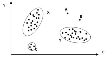Figure 1.1 Point anomaly [12]

1. OBJECTIVE

The prime objective is to allow more effective and efficient technique for predict credit fraud with use of anomaly detection, one in every of necessary use of anomaly detection during this thesis is to predict credit scoring default in loan or different financial sector. Anomaly Detection also known as Outlier detection is the method to find anomaly from data objects because its behaviors are terribly completely different from expectation. Such objects are known as outliers or anomalies. Anomaly detection is employed in several applications in equally to fraud detection like medical treatment, public safety and protection, detection of harm in industry, image processing, investigation of sensor/video, and intrusion detection. Anomaly detection and clustering analysis are 2 comparatively associated tasks. Cluster is employed for locating majority patterns in a data set and organizes the data accordingly, whereas anomaly detection makes an attempt to capture the ones terrific cases that deviate notably using the majority patterns. This thesis finds poorly explored area and attempts to propose a proper solution.

1.2 MOTIVATION

A credit score may be a statistical number that depicts a person’s trustiness. Lenders use a credit score rating to assess the probability that a person repays his owed. All the organizations will generate a credit score rating for every person by vicimisation the person’s preceding credit history. A credit score may be a 3-digit number range begins from 300 to 850, with 850 is the highest score that a borrower achieves. If the score of person is higher than the more financially trustworthy a person is considered to be. In simple language, a credit/loan default is given by an borrower have not made their agreed upon credit/loan payments to the lender. There are many varieties of reasons why a client may not have made payments, however a given period of time has passed, that non-payment record will become a part of the consumer’s credit history. After it becomes a part of the borrower’s credit history (or credit record) it is used during the formulation of the consumer’s credit score.

The majorities of tasks associated with credit fraud are created within the dark web websites and specialized to s different services in the dark web. These environments allow the flooding of illegal activities that related to the commercialization of stolen credit and debit cards and related information. The dark web represents a part of internet that is considered vital for the business of criminal crews that specialize in performing different fraudulent activities related to credit cards.

In the dark web different communities provide numerous things and illegal services, such as many amount of stolen card data, the codes that used for adjustment of payment systems (i.e. PoS, ATM), plastic, and card on demand services. In these dark web markets the offender will effortlessly gather and sell tools, illegal services and dataset that use for different types of illegal activities. The bank accounts opened with fake identities this fake account is then used for payment recipients for the sale of any type of product and service that related to credit card fraud.[13]

CHAPTER 2

DOMAIN INTRODUCTION

Big data could be a collective term for a multiple set technologies designed for storage, querying and analysis. Varied protests are in area in big data like storage, transition, visualization, searching, analysis, security and privacy violations and sharing. The epidemic growth of data altogether areas needs the progressive measures needed for manage and gain access to data, “Big data” define as the datasets size is above the performance of everyday database system to capture, save, manage, and also analyze. i.e., McKinsey&Company give definition of big data that they not define bigdata in terms of being larger than a certain range of terabytes (thousands of gigabytes). They supply assertion that, at the same time as generation advances through the years, the volume of data that increase as big data will also growth. Additionally the definition can differ by different zone, it depending on what kinds of system tools are normally available and what size of dataset is common in a appropriate industry. With the one caveats, big data in many area0 nowadays can vary from a number of terabytes to multiple petabytes (thousands of terabytes).

There are 4 properties associated with big data. The main aspects are Volume, Variety, Velocity, and Variability.

Volume: The size of big data is become very high as day to day. The data collected through social websites and sensor networks crosses petabytes to Zettabytes.

Variety: Data produced by different categories, it consist various kind of unstructured, standard, semi structured and raw data this data are very difficult to be handled by traditional systems.

Velocity: This is a concept which defines the speed at which the data generated and then become historical. This aspect is used for handle the incoming and outgoing data rapidly.

Variability: It describes the quantity of variance employed in summaries kept within the data bank and refers how they are spread out or closely clustered within the data set.

Figure 2.1 Big Data Properties

 

2.1 CHALLENGES IN ANOMALY DETECTION.

Defining a normal region which encloses every possible normal behavior is very though. Additionally the boundary between regular and anomalous behavior is often not specific. Thus an anomalous observation which lies close to the boundary can actually be normal, and vice-versa.

When anomalies are the end result of malicious actions, the malicious adversaries regularly adapt themselves to make the anomalous observations appear like regular, thereby making the task of defining normal behavior more though.

The exact plan of an anomaly is distinctive for one of kind domains. For example, in the medical a small alteration from normal (e.g., fluctuations in body temperature) might be an anomaly, even as comparable alteration in the stock market domain (e.g., fluctuations in the value of a stock) is most likely thought of as traditional. So applying a method developed for one domain to another isn’t always trustworthy.

Availability of classified data for training/validation of models used by anomaly detection techniques is typically a significant issue. —Often the data contains noise which tends to be similar to the actual anomalies and hence is hard way to distinguish and remove.

Figure 2.2 Anomaly detection technique approach

2.2 TYPE OF ANOMALY

2.2.1 POINT ANOMALIES: –

If an single data instance can be define as anomalous with respect to the other data, then the that point is known as a point anomaly. Point anomalies are the most effective type of anomaly and the focus of majority of research on anomaly detection. For example, in Fig. 1, point A and point B as well as point C in region are outside the boundary of the ordinary areas, and this reason that point is anomalies since they are distinct from normal data points. As a real life example, credit card fraud detection. Let the data set correlate to an individual’s credit card transactions, for the simplicity, assume that the data is defined using only one function: amount spent. A transaction for which the quantity spent is very excessive compared to the regular variety of expenditure for that individual can be point anomaly.[12]

2.2.2 CONTEXTUAL ANOMALIES: –

If a data item is anomalous in a specific context, then it is defined as a contextual anomaly also given as conditional anomaly. Notion of a context is brought on using the structure within data set and has to be specific as a part of the problem formulation. Every data example is defined using following two of attributes:

• Contextual attributes. The contextual attributes are used to determine the context (or neighborhood) for that instance. For example, in spatial data sets, the longitude and latitude of a place are the contextual attributes. In time collection data, time is a contextual characteristic that determines the placement of an instance on the entire series.
• Behavioral attributes. The behavioral attributes define the non-contextual characteristics of prevalence For example, in a spatial data set describing the common rainfall of the whole global; the amount of rainfall at any area is a behavioral attribute.[12] 

2.2.3 COLLECTIVE ANOMALIES: –

If a group of related data occurrence is anomalous with respect to the entire data set, it is termed as a collective anomaly. The individual data occurrences in a collective anomaly might not be anomalies by themselves; however their prevalence together as a group is anomalous.[12]

3. TECHNIQUES FOR ANOMALY DETECTION.

 

2.3.1 BAYESIAN NETWORK.

Bayesian belief networks are give joint conditional probability distributions. They give class conditional independencies to be described among subsets of variables. They give a graphical representation of causal relationships, on that the learning may be performed. This Bayesian networks is use for classification. Bayesian networks also referred as belief networks, Bayesian networks, and probabilistic networks. A belief network is defined with two components adirected acyclic graph and a conditional probability tables. Every node inside the directed acyclic graph gives a random variable. The variables could also be discrete-valued or continuous-valued. They may additionally measures to real attribute given inside the data or to “hidden variables” believed to form a relationship, for example, in the case of medical data, a hidden variable may imply a syndrome, representing a variety of syndrome that, together, characterize a particular disease. Each arc represents a probabilistic dependence. [15]

2.3.2 NEURAL NETWORK.

Neural networks exist in many ways and different forms. In this thesis we discuss a Feed Forward Multilayer Perceptron Network, this network consists of various00 layers of perceptron that area unit interconnected by asset of weighted connections it consist three layers:

Input layer: Receives value from input streams, which can be a database or some device or something else.

Hidden Layer: connects the network to the other input layer and receives in outside layer or only to the another hidden layer.

Output Layer: It connects with the Network with the outside world again and provides the final output of the network. The most effective example of neural network is given by the University of Saskatchewan; the researchers are using MATLAB and the Neural Network Toolbox model to determine whether a popcorn kernel can pop. [15]

2.3.3 SUPPORT VECTOR MACHINE.

SVM is another machine learning technique and its Generalization capacity is clearly higher than other learning techniques. This basic SVM manages two-class issues, known as Binary order problems in which the information are isolated by a hyper plane characterized by various support vectors. Support vectors are a subset of preparing information used to characterize the limit between the two classes. Every occurrence in the preparation set contains one “target esteem”. The target of SVM is to deliver a model that predicts target estimation of information.

In circumstances wherever SVM can’t separate two classes, it takes care of this issue by mapping input information into high-dimensional element spaces utilizing a portion work. In high-dimensional space it is conceivable to make a hyper plane that permits direct partition. Likewise, the portion work assumes an important part in SVM. The portion capacities can be utilized at the season of preparing of the classifiers which chooses support vectors on the surface of this capacity. SVM group information by utilizing these support vectors that framework the hyper plane in the element space. Practically speaking, different part capacities can be utilized, for example, linear, polynomial or Gaussian, SVM is used in bioinformatics, image classification, and hand-written character recognition. [16]

2.3.4 K-MEANS CLUSTERING.

The K-means clustering used for vector quantization, from signal processing, the aim of k-means clustering is to divide n observations into k clusters in which each operation fit to the cluster with nearest mean, serving a model of the cluster. Text mining includes extraction information from hidden patterns in big text-data collections. [15]

CHAPTER 3

LITERATURE REVIEW

1) A data-driven approach to predict default risk of loan for Online Peer-to-Peer (P2P) lending by Yu Jin, Yudan Zhu.[5]

This paper defines the feature selection method and also uses random forest method and gives attention to analysis propose the selected social and economic factors additionally to the bank typically used ones. This may help creditors understand the determinants of default risk. This Paper analyzes a massive dataset from the Lending Club, which is contrast to many prior studies which employ the data from Prosper. The data were collected from 2007 to 2011, this data include the effect of economic crisis in 2008 In this paper three kinds of DM models (DT, NN and SVM) and also use 10-fold cross validation and two classification metrics to evaluate the prediction results.[5]

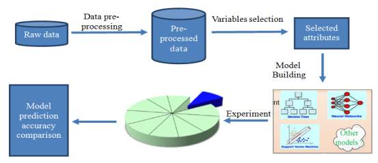Figure 3.1 Flow Graph for Default Prediction[5]

2) A Novel Graph-based Descriptor for the Detection of Billing-related Anomalies in Cellular Mobile Networks by Stavros Papadopoulos, Anastasios Drosou, and Dimitrios Tzovaras. [2]

This Paper presents a graph-based approach for the detection of billing-related anomalies in mobile networks. The technique uses graph-based descriptors to capture The network billing activity for a specific time period, where nodes in the graph represent users and/or servers, and edges represent communication events. This paper presents the method followed to create multiple graphs in each vertex neighbourhood of predefined size and presents the features that are extracted from the neighbourhood graphs for different neighbourhood sizes k, and used in order to train a supervised classification algorithm, namely, the Random Forest (RF) classifier, to recognize anomalous graphs.[2]

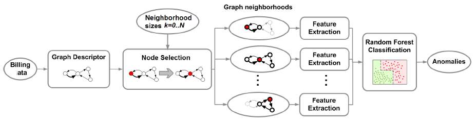Figure 3.2 Graph Based Descriptor[2]

Table 3.1 Anomaly Detection Rules[2]

#	Feature	Short description	Definition range	Anomaly detection
1	Volume	The number of edges of the Graph	K>=1	For identifying anomalies related to large unusually large network
2	Edge Entropy	The entropy of the weights of the edges in the graph	K>=1	Change in volume of data and change in their underling distribution.
3	Graph Entropy	Captures the structural characteristics of the graph Captures the structural characteristics of the graph	K>=1	This feature captures the behavior in which a malware initiates communication
4	Edge Weight Ratio	The ratio of the sum of weight of outward to inward edges	K>=0	Check spam SMSs on edge
5	Average Outward/Inward Edge weight	The average weights of the Outward/ Inward Edges The average weights of the Outward/ Inward Edges	K>=o	Neighbourhoods that include servers involved in an anomaly.

3) Anomaly Detection in Network Traffic Using K-mean clustering by R.Kumari, sheetansu, M.K. Singh, R.Jha, N.K. Singh.[1]

This paper represents a find anomaly in network using k-means clustering machine based approach with the use of big data analytical techniques and other approach is  to find the best results to prevent attacks at it’s very origin, in this paper they used a HDFS in spark shell they used R tools for visualization.[1]

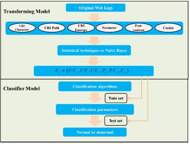
4) A Novel Anomaly Detection Approach for Mitigating Web-based Attacks against Clouds by Simin Zhang, Bo Li, Jianxin Li, Mingming Zhang, Yang Chen.[3]

This paper describes a transforming model that converts every entry into vector. Every value in the vector is a probability value, that is, every feature of each attribute is transformed to a corresponding value by statistical techniques or Naive Bayes. They propose a method to deal with URI without any query. It splits URI path string into tokens, so applies Naive Bayes to get their probability value. The detection system is carried out by a real-life dataset of millions of entries which is much larger than the datasets of prior study.[3]

Figure 3.3 Anomaly detection flow graph[3]

 

 

5) Modeling consumer Loan Default Prediction Using Neural Netware by Amira Kamil Ibrahim Hassan, Ajith Abraham.[4]

This paper give the comparison of three algorithms given by scaled conjugate gradient backpropagation, Levenberg-Marquardt and One-step secant backpropagation (SCG, LM and OSS). different parameters have been used for experiment to try and do the comparison; training time, gradient, MSE and R. The slow algorithm is OSS; the algorithm with the biggest gradient is SCG. The best algorithm is LM because it has the biggest R, this is  best for this dataset.[4]

Figure 3.4 Loan Default Prediction Process[4]

6) Identifying Features for Detecting Fraudulent Loan Requests on P2P platforms by Jennifer Xu, Dongyu Chen, Michael Chau.[6]

This exploratory examine is meant to deal the problem of fraudulent loan requests on peer-to-peer (P2P) platforms. They suggest a collection of alternatives that capture the behavioral characteristics (e.g., learning, past performance, social networking, and herding manipulation) of malevolent borrowers, who intentionally create loan requests to accumulate finances from lenders but default later on. They determined that using the widely adopted classification methods such as Random Forest and Support Vector Machines, the proposed feature set outperform the baseline feature set in helping detect fraudulent loan requests. Although the performance (e.g., Recall or Sensitivity) is still not up to its optimum, this study demonstrates that via analyzing the transaction records of confirmed malevolent borrowers, it is possible to capture some useful behavioral patterns for fraud detection. Such functions and techniques might probably help lenders identify loan request frauds and avoid financial losses. [6]

7) Machine Learning on Imbalanced Data in Credit Risk by Shiivong Birla, Kashish Kohli, Akash Dutta.[7]

This paper explains Credit Risk that described because the chance of loan default in the loan taken from a financial organisation. Threat is define by the shortage of primary principal and interest, disruption of money flows and improved collection charges. Loan Default associate uncommon phenomenon; henceforth they obtain the unbalanced data. They have adopted the approach of Logistic Regression also use Classification and Regression Trees (CART) with techniques including under sampling, Prior Probabilities, Loss Matrix and Matrix Weighing to address unbalanced records.[7]

8) Analysis on Credit Risk Assessment of P2P by Lei Xia and Jun-feng Li.[10]

P2P is a financial innovation, however it additionally faces few troubles, within the P2P lending market several non institutional debtors might be together. In a regular mortgage market, debtors must present their projects; lenders have to verify lending conditions and necessities. several of the loans has not dependent mortgage, Credit evaluation of the borrower is the most important task, in the absence of high quality data, the bank the right of investors under the right to the money to invest in the market activities, so one can abuse the current ideas of the new credit. Therefore, they suggest a model to evaluate the finding risk of default, based on the analysis, they could appropriatly assess the risk of default enhance return on investment.[10]

9) Credit default prediction modeling: an application of support vector machine

By Fahmida E. Moula Chi Guotai Mohammad Zoynul Abedin.[11]

Credit default prediction (CDP) modelling could be a basic and essential issue for financial institutions. However, the preceding studies imply that the classifier’s performances in CDP analysis take issue the usgae of distinct performance criterions on totally different databases below exceptional things. The  performance assessment exercising under a set of criteria remains understudied in nature, on the one hand, and the real–scenario is not taken consideration in that a single/very restricted quantity of measure only are used, on the other hand. These issues have an effect on the ability to make a consistent conclusion. Therefore, the intension of this study is to address this methodological issue by applying support vector machine (SVM)-based CDP algorithm by means of a set of representative performance criterions, with enclosing some novel performance measures, its overall performance examine with the consequences received through statistical and intelligent approaches using six totally different form  the credit prediction domains. Trial comes regarding demonstrate that SVM model is barely superior than CART with DA, being more hearty than its different partners.[11]

10) Analytics Using R for Predicting Credit Defaulters by Sudhamathy G. Jothi Venkateswaran C.[8]

The analysis of risks and assessment of default becomes crucial thereafter. Banks hold huge volumes of customer behaviour related data from which they are unable to arrive at a judgement if an applicant can be defaulter or not. Data Mining is a promising area of data analysis which aims to extract useful knowledge from tremendous amount of complex data sets. This work aims to develop a model and construct a prototype for the same using a data set available in the UCI repository. The model is a decision tree based classification model that uses the functions available in the R Package. before tobuilding the model, the dataset is pre-processed, reduced and made ready to provide efficient predictions. The final model is used for prediction with the test dataset and the experimental results prove the efficiency of the built model.[8]

 

Implementation step they prefer:-

Step 1 – Data Selection

Step 2 – Data Pre-Processing

Step 2.1 – Outlier Detection

Step 2.2 – Outlier Ranking

Step 2.3 – Outlier Removal

Step 2.4 – Imputations Removal

Step 2.5 – Splitting Training & Test Datasets

Step 2.6 – Balancing Training Dataset

Step 3 – Features Selection

Step 3.1 – Correlation Analysis of Features

Step 3.2 – Ranking Features

Step 3.3 – Feature Selection

Step 4 – Building Classification Model

Step 5 – Predicting Class Labels of Test Dataset

Step 6 – Evaluating Predictions.

11) Credit Risk Analysis in Peer-to-Peer Lending System by Vinod Kumar L, Natarajan S, Keerthana S, Chinmayi K M, Lakshmi N.[9]

The main aspect of this research is to analyze the credit risk that involved in P2P lending system of “LendingClub” Company. The Peer to Peer technique allows investors to get highest return on investment as compared to bank deposit, however it comes with a risk of the loan and interest not being repaid. Ensemble machine learning algorithms and preprocessing techniques are used to examine, analyze and conform the factors that play crucial role to predict the credit risk concerned in “LendingClub” 2013- 2015 loan applications dataset. A loan is examined “good” if it’s repaid with interest and on time. The algorithms are optimized to favor the potential good loans whilst identifying defaults or risky credits.[9]

 

CHAPTER 4

DATA DESCRIPTION

4.1 DATA DESCRIPTION

Advances in the development of P2P lending markets have provided large amounts of real-world P2P lending transaction data. study is based on public datasets from P2P lending marketplaces here I used the lending club data of 2014 whose consist the 2 lakh record of loan data in this data set I used the classification technique to find loan default, as a data pre-processing is perform for to remove NA value in data set after that the feature selection is perform.

Figure 4.1 Loan data of lending club

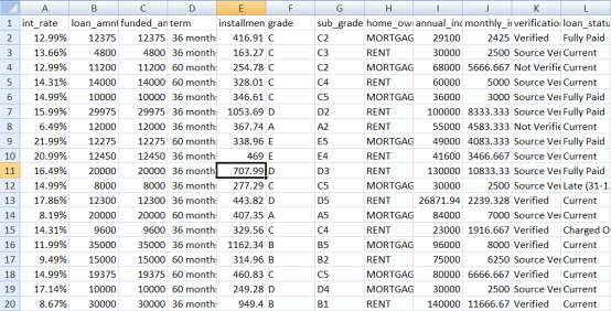
In data pre-processing first the missing value is finding by boruta package and the imputation done by PMM package, after cleaning and imputation process feature selection is done, feature is selected by random forest or correlation technique.

CHAPTER 5

PROPOSED METHODOLOGY

5.1 PROPOSED STATEMENT.

There are very less research done on credit scoring default with the use of data mining techniques but we use the Big Data techniques to predict best result. We use many paper for find best technique to predict anomaly in credit/loan data.

Flow graph for perform anomaly detection

Figure 5.1 Anomaly Detection Flow Graph

Figure 5.2 Flow Graph

5.2 PROPOSED WORK

Proposed work done with the implementation of base paper, in this implementation I used several classification model like Neural Network (NN), Decision Tree (DTs), Support Vector Machine (SVM), in the neural network the Multilayer Perceptron Network (MLP) is used for prediction and in decision tree Random Forest is used, I used the Lending Club Data to Analyzing it and to find loan defaulter using anomaly detection, here I compare the three model DT, NN, SVM for finding accuracy I  used  Confusion Matrix given in R Language, for Anomaly Detection I used linear regression model and logistic regression model, the data preparation is given below

5.2.1 DATA PREPARATION:-

Loan Status	Number Of loans	Percent
Default	30	0.1
Charged Off	2477	8.25
Late (31-120 days)	588	1.96
Late (16-30 days)	166	0.56
Current	18161	60.53
Fully Paid	8388	27.96

Table 5.1Loan status.

Table 5.2 Loan distribution by loan_ purpose

Purpose Of Loan	Total Number Of Loans	Percent
Debt consolidation	18380	61.27
Home Improvement	1534	5.113
Car	236	0.78
Credit Card	6737	22.46
House	106	0.35
Major Purpose	541	1.80
Medical	300	1
Moving	165	0.55
Other	1565	5.210
Small Business	270	0.9
Vacation	156	0.52

5.2.2 DATA CLEANING:-

There are 27 variables in loan data, First I did a data cleaning job in loan application almost there are all the column is complete but there one column that is in complete so I used imputing method to replace missing value, There is package called MICE (Multivariate Imputation By Chained Equations) in this package there is method called Predictive Mean Matching for imputation of missing value, the loan  database is given with loan information and personal information of loan

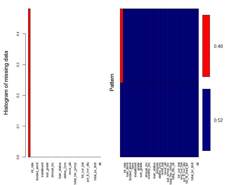Figure 5.3 Missing Data graph By VIM Package

NO.	Mths_since_last_delinq	dti
1	42	14.92
2	NA	12.02
3	60	18.49
4	NA	25.81
5	17	8.31
6	NA	39.79

NO.	Mths_since_last_delinq	dti
1	42	14.92
2	77	12.02
3	60	18.49
4	38	25.81
5	17	8.31
6	19	39.79

Table 5.3 Before imputation  Table 5.4 After imputation using MICE package

5.2.3 FEATURE SELECTION:-

In feature selection there is different method used but here I used the Random Forest and the Correlation method for feature selection. In R there is Boruta package that used for building a Random Forest tree for feature selection at the last it give the box plot graph of all the input variables if variable is correct than Boruta package give Confirmed statement if not it give rejected statement, after random forest selection I also used correlation function to perform feature selection the last selected variables is give below table.

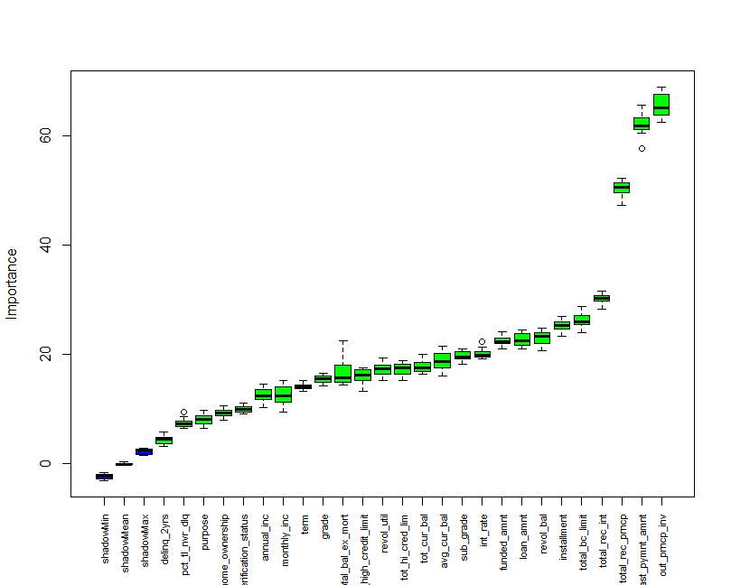      Figure 5.4 Boxplot graph for feature selection with BORUTA package

Variable	Attribute
int_rate	Interest rate on the loan
term	The number of payments on the loan. Values are in months 36 or 60.
grade	Loan grade
sub grade	Loan subgrade
revol_util	The amount of credit the borrower is using relative to all available revolving credit.
revol_bal	Total credit revolving balance
loan_amnt	The amount of the loan taken by the borrower
Installment	The monthly payment owed by the borrower if the loan originates.
annual_inc	The annual income of loan borrower
last_pymnt_amnt	Last total payment amount received
total_rec_int	Interest received to date
total_rec_prncp	Principal received to date
last_pymnt_amnt	Last payment amount received

Table 5.5 Selected variable using Random forest and correlation

 

 

 

 

 

 

 

 

 

 

 

 

 

 

 

 

 

 

5.2.4 DATA MODELING:-

In data modeling different classification/prediction model is used for example neural networks, decision trees, and support vector machine were build using the R for windows 3.3.2 and R studio 1.0.136, in this study, I used Random forest in decision tree. Neural network are the give best result for classification and prediction I used MLP (Multilayer Perceptron Network) for prediction of default loan, now the other approach is SVM (Support Vector Machine).  For data analysis there is different charts of model is generate using R language.

For simplicity I convert the Current and Fully_paid loan status with the Performing and other is converted into Non-performing type, the data analysis with graph is give below.

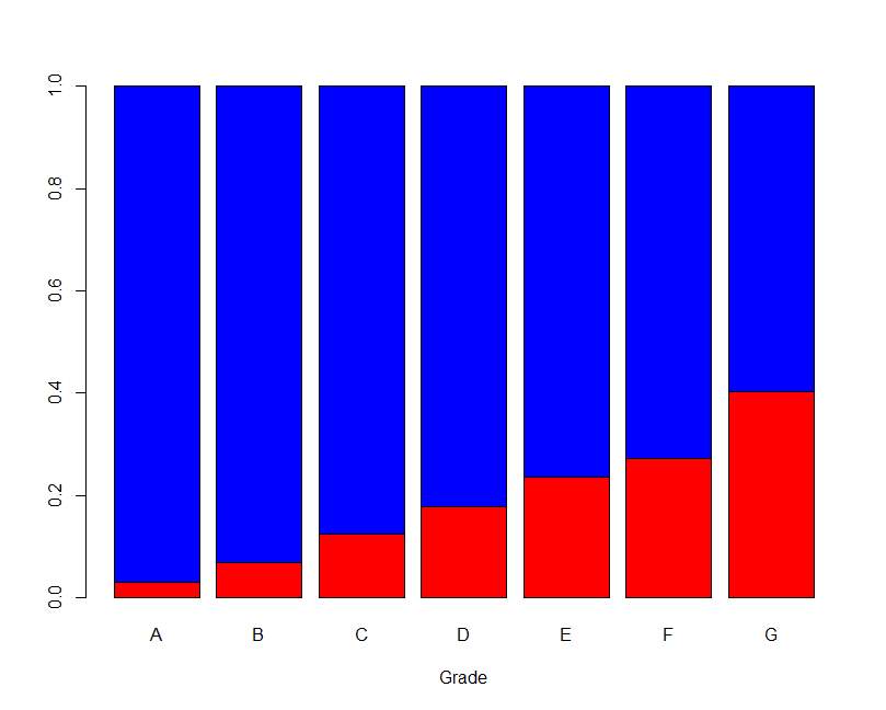
Var1	Var2	Freq.
Nonperforming	A	157
Performing	A	5091
Nonperforming	B	560
Performing	B	7635
Nonperforming	C	1060
Performing	C	7432
Nonperforming	D	858
Performing	D	3960
Nonperforming	E	559
Performing	E	1814
Nonperforming	F	194
Performing	F	520
Nonperforming	G	64
Performing	G	95

Figure 5.5 Bar plot of Loan Grade                                 Table 5.6 Loan grade frequency

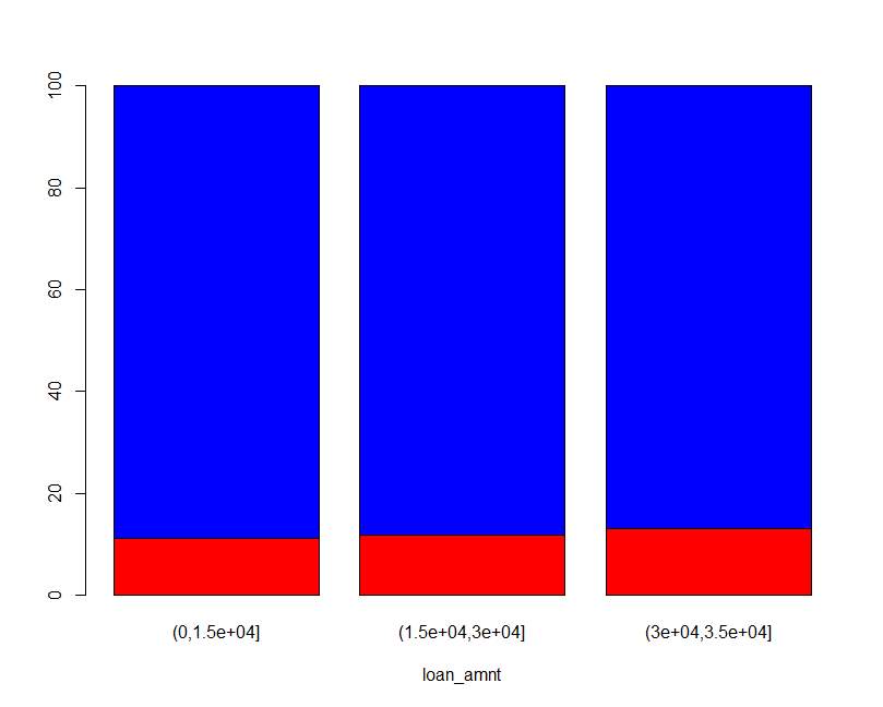
Var1	Var2	Freq.
Nonperforming	(0, 1.5e+04)	11.19
Performing	(0, 1.5e+04)	88.81
Nonperforming	(1.5e+04, 3e+04)	11.77
Performing	(1.5e+04, 3e+04)	88.23
Nonperforming	(3e+04, 3.5e+04)	13.04
Performing	(3e+04, 3.5e+04)	86.96

Figure 5.6 Bar plot of Loan amount                           Table 5.7 Loan amount frequency

In the loan data the delinquencies in the past 2yrs has value from 0 to 22 so here I take value 0, 1, and 2 and for 3 to 22 I used 3+ as shown in graph.

Table 5.8 Delinquencies frequency

Figure 5.7 Bar plot of  delinquencies

Var1	Var2	Freq.
Nonperforming	0	11.23
Performing	0	88.77
Nonperforming	1	12.91
Performing	1	87.09
Nonperforming	2	12.09
Performing	2	87.91
Nonperforming	3+	11.75
Performing	3+	88.25

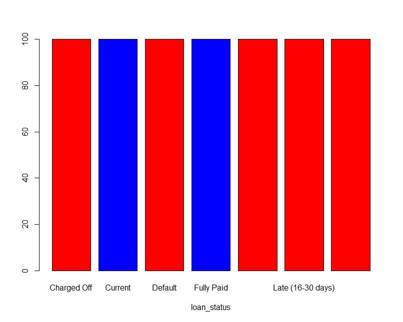
Var1	Var2	Freq.
Nonperforming	Charged Off	100
Performing	Charged Off	0
Nonperforming	Current	0
Performing	Current	100
Nonperforming	Default	100
Performing	Default	0
Nonperforming	Fully Paid	0
Performing	Fully Paid	100
Nonperforming	In Grace Period	100
Performing	In Grace Period	0
Nonperforming	Late (16-30 Days)	100
Performing	Late (16-30 Days)	0
Nonperforming	Late (31-120 Days)	100
Performing	Late (31-120 Days)	0

Figure 5.8 Bar plot of loan_status                           Table 5.9 loan_stauts frequency

CHAPTER 6

SIMULATION AND RESULT

In this study I perform MLP, decision tree and support vector machine for prediction of the loan default and I also perform the anomaly detection using the linear regression all the simulation graph is given below.

6.1 PERFORMANCE MEASURES

The classifier is appraising based on the confusion matrix. The Predicted delicacy is in the column and the Actual class is in the row. A confusion matrix have 4 components on which our classifier is evaluated on, specifically, TN define by negative cases that are classified correctly (True Negatives), FP define by negative cases that are classified incorrectly as positives (False Positives), TP define by positive cases that are correctly classified (True Positives) and FN define by positive cases which are incorrectly classified as negative (False Negatives). Prediction Accuracy is typically defined.

		Predicted
		x	y
Actual	x	TN	FP
	y	FN	TP

Table 6.1 Confusion Matrix

6.2 SUPPORT VECTOR MACHINE

Table 6.2 Confusion matrix table for SVM

		Reference
		Nonperforming	Performing
prediction	Nonperforming	2	34
	Performing	45	418
Accuracy :84%

 

6.3 MULTI-LAYER PERCEPTRON NETWORK

Figure 6.1 Graph for MLP

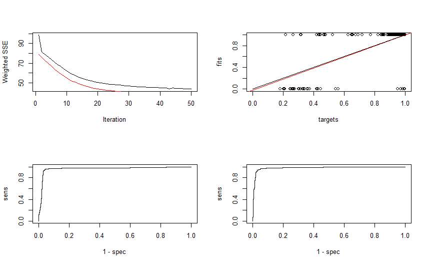
Table 6.3 Confusion matrix table for MLP

		Reference
		Nonperforming	Performing
prediction	Nonperforming	33	11
	Performing	13	443
Accuracy :85%

6.4 ANOMALY DETECTION

The liner regression graph for anomaly detection is given below, the linear regression graph is for monthly_income vs. installment now here I give the regression graph of the 200 value for simplicity. Now the anomaly is detected using by simple probability. If the monthly income of borrower is less but it take the highest loan than it likely to be perform default.

6.4.1 LINEAR REGRESSION

Linear regression is used for to find the relationship between the two variables used for find best fit the value of linear function. The linear regression graph for the data is given below.

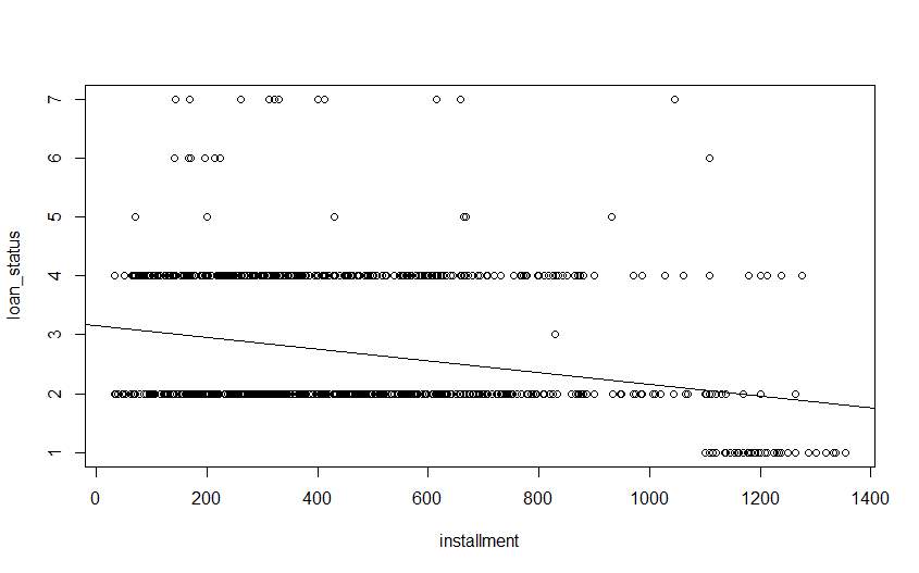Figure 6.2 Linear Regression Graph installments vs. Loan_status

As shown in above figure the plot of installment vs. loan_status with linear regression The blackline is the abline that adds the line using the generated linear model in R now as our probability here,  the above graph we can see that the installment with higher than 1000 Is perform charged off no for that I made one algorithm that give number of total borrower that perform default during it loan period.

Steps For Find Anomaly

Step 1 – Select set of n records

Step 2 – create Subset s1 where charged off/default = TRUE

Step 3 – create subset s2 where charged off/default =FALSE

Step 4 – calculate mean of s1 as Ms1

MS1=mean (s1)

Step 5 – calculate mean of s2 as Ms2

Ms2=mean(s2)

Step 6 – find difference of Ms1 and Ms2

D = Diff (Ms1, Ms2)

Step 7 – calculate Ms from original data

Ms=mean(Data)

Step 8 – X = ifelse (Ms > D , Ms, D)

Step 9 –  for find Y repeat step 5 to 8

Step 10 – Y = ifelse (Ms > E , Ms, E)

Step 11– ifelse (installment > X, loan_status == Charged Off/Default)

ifelse (monthly_inc > X, loan_status == Charged Off/Default)

ifelse (monthly_inc > X, installment < Y, loan_status == Charged Off/Default)

Using Above steps to find the anomaly in loan data.

Rule 1: DF <- ifelse(data$installment >= X & data$loan_status == “Charged Off”, ”  Charged off”, “not charged off”)

In above rule the value X is used  now as the given rule if installment is greater than or equal to/less than or equal to X and the loan status is “Charged Off “ than it give the  anomaly in loan data.

Table 6.4 Classified Value Table for Installment Vs. Loan_status

Data with (1000 Rows)	Mean Value(Ms1)	Mean Value(Ms2)	Ms	Actual	Classified
Part1	1207.32	414.50	466.08	65	64
Part2	1006.77	447.29	492.05	80	80
Part3	896.62	426.02	451.73	58	56
Part4	799.61	450.20	421.94	91	86
Part5	732.83	421.94	448.03	84	83

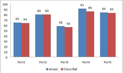Figure 6.3 Comparison Chart of Installment Vs. Loan_status for Actual And Classified Value.

 

 

 

 

 

 

 

 

 

 

 

Table 6.5 Classification Table for Installment Vs. Loan _status

Rows	Classification
1	Not Charged Off
2	Not Charged Off
3	Not Charged Off
4	Not Charged Off
5	Charged Off

Rule2: DF <-ifelse(data$monthly_inc <= Y & data$installment >= X & data$loan_status == “Charged Off”, “Charged off”, “not charged off”)

In above rule the value of X  and Y used as the given rule if installment is greater than or equal to X and the monthly-inc is less than the Y and  loan status is “Charged Off “ than it give the  anomaly in loan data

Table 6.6 Classified Value Table for Monthly_inc vs. Installment vs. Loan_status

Data with (1000Rows)	Actual	Classified
Part1	65	12
Part2	80	28
Part3	58	14
Part4	91	41
Part5	84	43

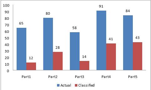Figure 6.4 Comparison Chart of monthly_inc Vs. Installment Vs. Loan_status for Actual And Classified Value.

Table 6.7 Classification Table monthly_inc vs. Installment vs. Loan_stauts

Rows	Classification
1	Not Charged Off
2	Not Charged Off
3	Not Charged Off
4	Not Charged Off
5	Not Charged Off

Rule3: DF <-ifelse(data$monthly_inc >= X & data$loan_status == “Charged Off”, “Charged off”, “not charged off”)

In above rule the value Y is used  now as the given rule if  monthly_inc is greater than or equal to/less than or equal to Y and the loan status is “Charged Off “ than it give the  anomaly in loan data .

Table 6.8 Classified Value Table for monthly_inc Vs. Loan_status

Data with (1000 Rows)	Mean Value(Ms1)	Mean Value(Ms2)	Ms	Actual	Classified
Part1	10655.79	6530.94	6799.32	65	52
Part2	10173.88	7063.46	7312.30	80	52
Part3	9110.76	6355.46	6515.73	58	42
Part4	8660.27	6646.66	6829.90	91	45
Part5	7229.26	6448.24	6513.85	84	43

 

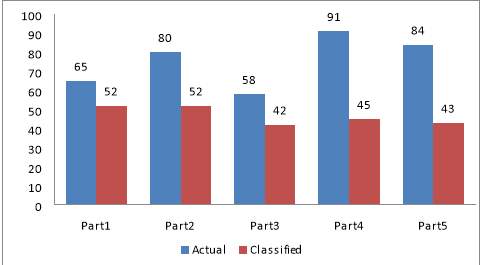Figure 6.5 Comparison Chart of monthly_inc Vs. Loan_status for Actual And Classified Value.

Table 6.9 Classification Table for monthly_inc Vs. Loan_status

Rows	Classification
1	Not Charged Off
2	Not Charged Off
3	Not Charged Off
4	Not Charged Off
5	Not Charged Off

6.4.2 LOGISTIC REGRESSION

 

The .logistic regression is used to estimate the probability of binary response based on one or more predictor variables.

Probability equations of logistic regression is

Probability =

1/(1+e^((coefficient*X+intercept)) )

 

Figure 6.6 Fitted Value Chart for Logistic regression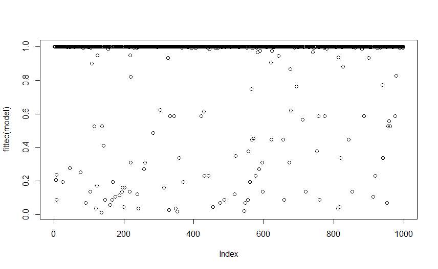

Now Find Fitted value for loan data the below given tables is give the fitted value for loan_status Vs.  Installment.

Table 6.10 Comparison Chart for Actual And Classified Value

Loan_status Vs. Installment

Data with (1000 Rows)	Actual	Classified
Part1	65	69
Part2	80	61
Part3	58	20
Part4	91	25
Part5	84	17

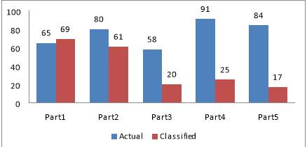Figure 6.7 Comparison Chart for Actual And Classified Value

For Logistic regression

Table 6.11 Comparison Chart for Actual And Classified Value

Loan_status Vs. Monthly_inc

Data with (1000 Rows)	Actual	Classified
Part1	65	15
Part2	80	3
Part3	58	2
Part4	91	1
Part5	84	0

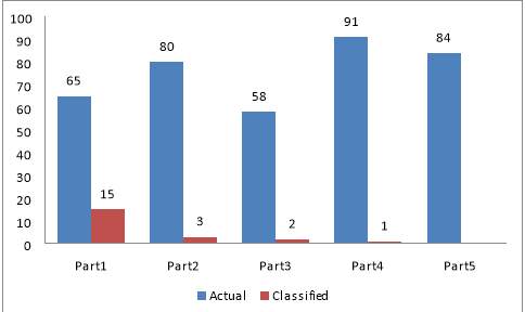Figure 6.8 Comparison Chart for Actual And Classified Value for Logistic regression

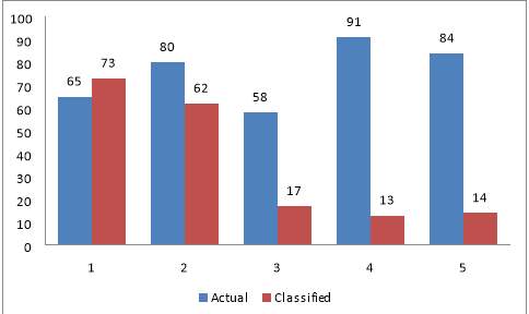
Table 6.12 Comparison Chart for Actual And Classified Value

Loan_status Vs. Monthly_inc Vs. Installment

Data with (1000 Rows)	Actual	Classified
Part1	65	73
Part2	80	62
Part3	58	17
Part4	91	13
Part5	84	14

Figure 6.9 Comparison Chart for Actual And Classified Value for logistic regression  

6.4 COMPARISON CHART

 

The Given Below figure shows that rule based classifier is more accurate as compare to logistic regression.

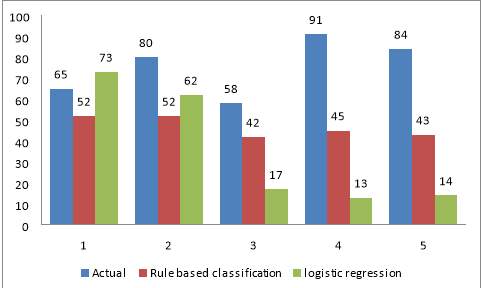Figure 6.10 Comparison Chart for Logistic regression vs. Rule based classification

 

The Given Below figure shows that rule based classifier is more accurate as compare to logistic regression

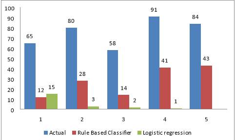Figure 6.11 Comparison Chart for Logistic regression vs. Rule based classification

The Given Below figure shows that rule based classifier is more accurate as compare to logistic regression

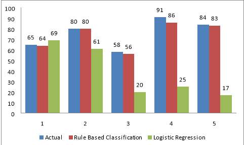
Figure 6.12 Comparison Chart for Logistic regression vs. Rule based classification

So as compare to logistic regression the Rule based give more accurate classification of the

Loan defaulter, using this rule user can also find future prediction that the borrower is likely to be perform default.

CHAPTER 7

CONCLUSION

Concerning about find credit/loan default that give creditworthiness about the person or organization. In this thesis I briefly review about the big data, anomaly detection and the different techniques like MLP and SVM for prediction of the loan default, here I give the comparison of MLP and SVM models for loan data, after comparing two models the MLP give the best result for prediction loan default. Now for the anomaly detection I give the linear regression to perform the classification, for perform classification the algorithm is made using the three rule the all rule give the classified data from the loan the comparison chart also given, the logistic regression is also perform for comparing classified data as per comparison with logistic regression and rule based classification the rule based classification is give much better result as compared to logistic regression.

CHAPTER 8

REFERENCES

1. R. Kumari, Sheetanshu, M. K. Singh, R. Jha and N. K. Singh, “Anomaly detection in network traffic using K-mean clustering,” 2016 3rd International Conference on Recent Advances in Information Technology (RAIT), Dhanbad, 2016, pp. 387-393.
   doi: 10.1109/RAIT.2016.7507933.

2. S. Papadopoulos, A. Drosou and D. Tzovaras, “A Novel Graph-Based Descriptor for the Detection of Billing-Related Anomalies in Cellular Mobile Networks,” in IEEE Transactions on Mobile Computing, vol. 15, no. 11, pp. 2655-2668, Nov. 1 2016.
   doi: 10.1109/TMC.2016.2518668

3. S. Zhang, B. Li, J. Li, M. Zhang and Y. Chen, “A Novel Anomaly Detection Approach for Mitigating Web-Based Attacks Against Clouds,” 2015 IEEE 2nd International Conference on Cyber Security and Cloud Computing, New York, NY, 2015, pp. 289-294. doi: 10.1109/CSCloud.2015.46

4. K. I. Hassan and A. Abraham, “Modeling consumer loan default prediction using neural netware,” 2013 INTERNATIONAL CONFERENCE ON COMPUTING, ELECTRICAL AND ELECTRONIC ENGINEERING (ICCEEE), Khartoum, 2013, pp. 239-243. doi: 10.1109/ICCEEE.2013.6633940

5. Y. Jin and Y. Zhu, “A Data-Driven Approach to Predict Default Risk of Loan for Online Peer-to-Peer (P2P) Lending,” 2015 Fifth International Conference on Communication Systems and Network Technologies, Gwalior, 2015, pp. 609-613.
   doi: 10.1109/CSNT.2015.25

6. J. Xu, D. Chen and M. Chau, “Identifying features for detecting fraudulent loan requests on P2P platforms,” 2016 IEEE Conference on Intelligence and Security Informatics (ISI), Tucson, AZ, 2016, pp. 79-84.
   doi: 10.1109/ISI.2016.7745447

 

7. S. Birla, K. Kohli and A. Dutta, “Machine Learning on imbalanced data in Credit Risk,” 2016 IEEE 7th Annual Information Technology, Electronics and Mobile Communication Conference (IEMCON), Vancouver, BC, 2016, pp. 1-6.
   doi: 10.1109/IEMCON.2016.7746326

8. G. Sudhamathy and C. J. Venkateswaran, “Analytics using R for predicting credit defaulters,” 2016 IEEE International Conference on Advances in Computer Applications (ICACA), Coimbatore, 2016, pp. 66-71. doi: 10.1109/ICACA.2016.7887925.

9. Vinod Kumar L, Natarajan S, Keerthana S, Chinmayi K M and Lakshmi N, “Credit Risk Analysis in Peer-to-Peer Lending System,” 2016 IEEE International Conference on Knowledge Engineering and Applications (ICKEA), Singapore, 2016, pp. 193-196. doi: 10.1109/ICKEA.2016.7803017

10. Lei Xia and Jun-feng Li, “Analysis on Credit Risk Assessment of P2P” 2016 E. Qi et al. (eds.), Proceedings of the 22nd International Conference on Industrial Engineering and Engineering Management 2015, DOI 10.2991/978-94-6239-180-2_86

11. Fahmida E. Moula, Chi Guotai, Mohammad Zoynul Abedin, “Credit default prediction modeling: an application of support vector machine”, DOI 10.1057/s41283-017-0016-x

12. Chandola, V., Banerjee, A., and Kumar, V. 2009. Anomaly detection: A survey. ACM Comput. Surv. 41, 3, Article 15 (July 2009), 58 pages. DOI = 10.1145/1541880.1541882

13. http://www.investopedia.com/terms/d/defaultrisk.asp .

14. Jiawei Han, Micheline Kamber, Jian Pei, “Data Mining Concept and Techniques”.

15. Sam Maes, Karl Tulys, Bram Vanschoenwinkel, Bernard Manderick, “credit card Fraud Detection. Applying Bayesian and Neural Network”, 2016.

16. Ravinder Reddy, B.kavya, Y Ramadevi (Ph.D.), “A Survey on SVM Classifier for Intrusion Detection”, 2014.