Response of a Reinforced Concrete Structure to Different Loads

CHAPTER 1

 INTRODUCTION

1.1 GENERAL

In this age of technology, studies on materials are being done at micro as well as nano levels. Concrete has been regarded as a low tech and well understood material. However, concrete being the second most consumed material in the world, an impressive amount of research has been carried out over the last century and the studies are being pursued, in order to understand the phenomenon and mechanisms that are governing its complex behaviour. The complex macroscopic behaviour and failure mechanisms of concrete can be determined by observing the heterogeneous structure at nano, micro and meso levels. And in fact, still today, there is plenty of scope for exploring the fundamental nature of concrete and its behaviour.

Nowadays, for detailed studies of materials, we usually go for mathematical models. Mathematical models currently available for concrete are, as yet incapable of reproducing the mechanical behaviour as well as transient behaviour of this material in a very accurate manner. Even though different mathematical models are available, long-standing issues regarding concrete complexities remain to this day. One such aspect is modelling the mechanical behaviour of concrete. The lack of a widely accepted and accurate mathematical model for predicting the mechanical behaviour of concrete in practice prevents the widespread use of non linear analysis of concrete structures. This may also pose a hindrance to the development of the new research areas on concrete.

Concrete modelling can be classified into two main categories at a constitutive level, macroscopic model that follows a phenomenological approach and models based on micromechanical solutions. Phenomenological models generally employ theories based on plasticity or damage mechanics for simulating the macroscopic behaviour. On the other hand micromechanical models aim to relate the microstructure of concrete, and the physical mechanisms that govern its evolution, to the macroscopic behaviour observed in experiments.

This study addresses such a numerical model called microplane formulation. It lately became more and more popular for the delineation of quasi-brittle materials. The substantive feature of this material model is the separation of local microplane strains and stresses allowing one to resort to simplified or in certain cases even unidirectional constitutive laws. The main charm of the microplane concept is that it can describe an initial or evolving anisotropic material behaviour in a simple as well as natural way. From the macroscopic point of view, it is recommended to restrict the microplane concept to the split of stresses into pure volumetric and deviatoric part, as a constraint subset of the most often used volumetric-deviatoric-tangential split. The particular advantage of volumetric-deviatoric split is that typical macroscopic responses are directly reflected on the mesoscale. In certain cases microplane modelling is closely related to well known macroscopic models even though microplane formulation seems to be much more general than those macroscopic formulations.

1.2 OBJECTIVES

• To use microplane model numerical analysis of reinforced concrete beams in ANSYS.
• To predict the flexural behaviour of a reinforced concrete beam using microplane model.
• To study the flexural behavior and crack simulation for reinforced concrete deep beam using microplane model.
• To conduct a parametric study using different L/D ratios (1.5, 1.6, 1.71) and longitudinal reinforcement ratios (0.5, 1, 1.5, 2) on the shear strength of RC deep beams.
  3.  SCOPE

The scope of the study is to predict the response of a reinforced concrete structure to different loads by using microplane plane model, as different models are being used nowadays for reinforced concrete members. The main attraction of the microplane concept is that an initial or evolving anisotropic material behavior can be described in a natural and simple way.

 

1.4 METHODOLOGY

• Validation by modelling an RC beam as per “Flexural Behaviour of RCC Beams” done by S. Tejaswi, 2015.

• Use of microplane modelling for the analysis of reinforced concrete beam using ANSYS.
• Analysis of reinforced concrete beam using microplane model for understanding its flexural behaviour.
• Analysis of a reinforced concrete deep beam using microplane model for simulating flexural behaviour and cracking patterns for different l/d ratios, 1.5, 1.6, 1.71.

 

 

 

 

 

 

 

 

 

 

CHAPTER 2

 LITERATURE SURVEY

Extensive researches and studies have been carried out for the last few decades and are being pursued in order to model and explain behaviour of quasi-brittle materials such as concrete. It is widely accepted and recognized that the heterogeneous structure of materials to be observed and studied at nano, micro and meso levels for understanding their complex macroscopic behaviour as well as failure mechanisms.

Beleandez et al., (2003) studied the classical problem of deflection of a cantilever beam, under the action of a uniformly distributed load along its length (its own weight) and an external vertical concentrated load at the free end. The beam was of linear elastic material and the problem was analyzed experimentally and numerically.

They presented the differential equation governing the behaviour of this system and showed that this equation is in fact rather difficult to solve due to the presence of a non linear term. The experiment described in this study is an easy way to introduce the concept of geometric nonlinearity in mechanics of materials. Finite element software ANSYS has been used to numerically evaluate the system and to calculate the Young’s modulus of beam material. Finally, they have compared the numerical results with the experimental ones obtained in the laboratory.

Hayder Qais Majeed, (2012) presented a nonlinear finite element modelling of steel fiber reinforced concrete (SFRC) deep beams and analysis of the same with and without openings in web. Beams taken for this study were subjected to two-point loading. In this study, ANSYS nonlinear finite element software has been used. Steel fiber percentage was varied from 0 to 1%.The effect of fiber content in the case of SFRC deep beams has been studied by measuring the deflection at mid span and by obtaining the cracking patterns. For the deep beams, with and without openings and with different steel fiber ratios, failure loads were obtained along with shear stresses and first principal stresses.

From this study, it was drawn that the location of openings as well as the amount steel fiber affects the strength and behaviour of deep beams. Results obtained from the deep beam modeled using ANSYS finite element program were compared with the results of the experiments taken from the literature, and it was shown that the results of analytical model is giving similar results to the experimental behaviour.

Honggun Park and Hakjun Kim, (2003) studied microplane models for the analysis of two dimensional planar members and three dimensional members in which three dimensional spherical microplanes has been used. And it seemed, to not accurately simulate the post cracking behaviour of reinforced concrete in tension-compression. In this study, Honggun Park and Hakjun Kim developed a new microplane model to overcome these disadvantages. They proposed a microplane model that uses disk microplanes with a lesser number of microplanes and two-dimensional stresses and strains in the place of existing spherical microplanes. And the proposed model was found to be more effective in numerical calculation. Also, strain boundary concept has been introduced to accurately describe the compressive behaviour of reinforced concrete with tensile cracks in tension-compression. The validity of the proposed model was verified by comparing it with experiments. Details of microplane model and the numerical technique involved in the finite element analysis have also been discussed comprehensively.

Iulia C Mihai, (2012) demonstrated the potential of micromechanical models to finally achieve a fully robust and comprehensive model for concrete, as considerable amount of researches and studies has been carried out for developing models since 1960’s and techniques seemed to not effectively simulating the mechanisms leading to failure of quasi-brittle materials such as concrete.

Even though significant progress was achieved during this time, not one numerical model showed ability to fully capture all the steps and facets in the complex mechanical behaviour of concrete. But the author has not developed a definitive model as such in this study. He vividly demonstrated the potential of the models developed till then and represented a significant step forward in the use of micro-mechanical theories for the constitutive modelling of concrete as he gave a particular focus to the development of a micromechanical constitutive model.

Author adopted a more mechanistic approach for his model where a number of phenomenological aspects of the previous numerical formulations were replaced with mechanistic components. Based on the classic Eshelby inclusion solution, author has adopted a two phase composite elasticity theory to simulate a composite material. It comprises of an elastic matrix and spherical inclusions to simulate the mortar and coarse aggregate particles respectively.

Author addressed micro cracking in the elastic matrix by evaluating the added compliance from the distribution of cracks with various orientations. A micro crack initiation criterion has been proposed, which employs the exterior point Eshelby solution to capture the tensile stress concentrations in the vicinity of the matrix-inclusion boundary. Micro cracks were assumed to initiate in the interfacial transition between coarse aggregate particles and mortar. Numerical predictions were compared against experimental results for a range of uniaxial, biaxial and triaxial simulations in order to assess the performance of the proposed model at a constitutive level.

Josko Ozbolt et al., (2015) studied the static and dynamic fracture of steel by modelling and analyzing a compact tension specimen (CTS), which is loaded under loading rates up to 100  m/s. Behaviour of structures and materials strongly depends on the loading rate. Structures loaded by high loading rate and impact acts in a different way compared to quasi-static loading. After loading, at first, there is a strain rate influence on strength, stiffness, and ductility, and, second, inertia effect gets activated. These effects can be clearly shown by experiments. Even though steel does not exhibit significant strain rate sensitivity; the dynamic fracture of steel seemed to be highly sensitive on loading rates.

Here, in this, author has proposed a microplane model for steel. Later on it was verified for monotonic and cyclic quasi-static loading. After that, three-dimensional (3D) finite element dynamic fracture analysis is carried out. It is shown that the resistance of steel, apparent strength and toughness, increases progressively after the critical strain rate (approximately 100/s) is reached. Then, crack branching phenomena and significant ductility decrease were observed.

The phenomenon which was well known from experimental evidence was attributed to the effect of structural inertia and inertia related to high nonlinear behaviour of steel at the crack tip in the plastification zone. The numerical results indicated that maximum crack velocity of steel is much lower than the Rayleigh wave velocity, and for the investigated steel, it reached approximately 400 m/s.

Maurizio et al., (2005) investigated the shear behaviour of concrete beams with fiber reinforced polymer (FRP) as reinforcement. Two successive phases of testing were done on six beams. Three beams were reinforced with conventional steel reinforcement for flexure and the other three were reinforced with glass fiber bars. Study was conducted for different shear span to depth ratios, ranging from 1.1 to 3.3.Modelled beams were analyzed, in order to study the difference in the shear behaviour of beams due to different types of shear failure.

In the first phase of testing, no shear reinforcement was provided and in the second phase of testing, to enable failure due to shear, just sufficient glass and carbon fiber shear reinforcement was provided. Later, predictions were made according to the design recommendations based on ACI and the Institution of Structural Engineers; U.K. Test results when compared with the predictions showed that these approaches, based on modifications of equations derived for steel reinforcement, underestimate the contribution of the concrete and the shear reinforcement to the total shear capacity of FRP reinforced concrete beams. It was also shown that both approaches could be modified to become less conservative.

Michael Leukart and Ekkehard Ramm, (2006) addressed the so called numerical model namely microplane model for the description of quasi-brittle materials. The important feature of this model is a split of the local microplane strains and stresses. It allows one to resort to simplified stress-strain relationship or in certain cases even unidirectional constitutive laws.

From the macroscopic viewpoint, it is recommended to restrict the microplane concept to the pure volumetric-deviatoric split which is a constraint subset of the most often applied volumetric-deviatoric-tangential split. Volumetric-deviatoric split has the particular advantage that typical macroscopic responses are directly reflected on the mesoscale.

It was also shown that in certain cases the present version of a microplane formulation is closely related to well-known macroscopic models although being much more general than those macroscopic formulations. This close relation is exploited to derive physically sound microplane constitutive laws. Identification and interpretation of the microplane constitutive laws was done by the comparison of the microplane formulation to a well-known macroscopic one-parameter damage model and the constitutive formulations are embedded in a thermodynamically consistent framework.

Moufaq Noman Mahmoud, (2007) mainly concentrated on finding the most economical way to design deep beams in this study, as these are being widely used as structural elements in building construction. Stiffness of the deep beam is very high and it has different uses. For example, deep beams can be used to distribute the loads of a building on the piles below or to prevent relative movement or settlement. A common problem in these structures is clearly visible cracks in serviceability conditions. This has its effect on the durability and on the aesthetics of the structure.

In order to study these problems, challenging deep beams have been investigated; deep beams with rectangular shapes, special shapes and also with different kinds of openings. The obtained result has also been used to validate the design methods. This exposed possible weaknesses in both code compliance and clarity of the design process. Later recommendations were proposed to the design procedures based on the study. An advice for obtaining a better method for designing deep beams was also given this study.

P.Bazant et al., (1988) calibrated the general microplane model formulated and verified by comparison with numerous non linear triaxial test data from the literature. And the comparison showed good agreement. This model involved only fewer material parameters than the previous phenomenological macroscopic models. Numerical implementation has also been considered in this study.

P.Bazant et al.,(1992) used microplane constitutive model for non linear triaxial behaviour and fracture of concrete in nonlocal finite element analysis of compression failure in plane strain rectangular specimens. The loading path is divided into two at the beginning of post-peak softening for specimens with sliding rigid platens. A primary path exists, but the stable path is the secondary path, involving an inclined shear expansion band that consists of axial splitting cracks and is characterized by transverse expansion.

The secondary path is indicated by the first Eigen value of the tangent stiffness matrix but can be more easily obtained, if a slight non symmetry is introduced into the finite element model. In specimens with bonded rigid platens there is no bifurcation; they fail symmetrically, by two inclined shear expansion bands that consist of axial splitting cracks. It was found that the transverse expansion produced transverse tension in the adjacent material, which served as the driving force of propagation of the axial splitting cracks. Also, numerical calculations indicated no significant size effect on the nominal stress at maximum load.

P.Bazant et al., (1999) extended study for the formulation of the microplane model for concrete and development of model M4 to large strains in this study. At first he cited some examples of certain difficulties with the second Piola-Kirchhoff stress tensor in the modelling of strength and frictional limits on weak planes within the material and the back-rotated Cauchy (true) tensor was introduced as the stress measure.

The strain tensor conjugate to the back-rotated Cauchy stress tensor is unsuitable because it is path dependent and its microplane components do not characterize meaningful deformation measures. Therefore Green’s Lagrangian tensor was adopted, even though it was not conjugate. The microplane components of the strain tensor suffice to characterize the normal stretch only for this strain measure and shear angle on that microplane. Using of such non conjugate strain and stress tensors seemed to be admissible for concrete because the elastic parts of strains as well as the total volumetric strains were always small. And also the algorithm used guaranteed the energy dissipation by large inelastic strains to be non-negative.

P. Bazant et al., (2000) presents an improved microplane constitutive model for concrete, representing the fourth version in the line of microplane models. The constitutive law was characterized as a relation between the normal, volumetric, deviatoric, and shear stresses and strains on planes of various orientations, called the microplanes. The strain components on the microplanes are the projections of the continuum strain tensor. Then the continuum stresses are obtained from the microplane stress components by principle of virtual work.

The improvements included a work conjugate volumetric – deviatoric split, additional horizontal boundaries (yield limits) for the normal and deviatoric microplane stress components, an improved non linear frictional yield surface with plasticity asymptote, a simpler and more effective fitting procedure with sequential identification of material parameters, a method to control the steepness and tail length of post peak softening and damage modelling with a reduction of unloading stiffness and crack closing boundary facilitating  physical interpretation of stress components.

P. Bazant et al., (2000) represents an explicit numerical algorithm for microplane model M4. The material parameters of model M4 were calibrated by optimum fitting of the basic test data available from the literature, and the model was verified by comparison with these data. The data in which strain localization must have occurred were delocalized, and the size effect was filtered out from the data wherever necessary. Although model M4 contained many material parameters, all but four have fixed values for all types of concretes. Thus the user needs to adjust only four free material parameters to the data for a given concrete and for that a simple sequential identification procedure was developed.

S. Ismail et al., (2016) provides an extensive numerical investigation on the role of key parameters on the shear performance of RC deep beams using the M4 microplane material model. Even though much work has been made on the shear behaviour of RC elements, design provisions available are based on empirical data and their predictions, especially for deep beams. These are not always reliable and can lead to unconservative results. The model was validated against experimental results of 20 RC deep beams. A parametric study was then carried out to investigate the effect of shear span to depth ratio and concrete compressive strength for RC deep beams with and without shear reinforcement. Although a single strut mechanism is generally mobilized in deep beams, the presence of shear reinforcement can enable a more uniform distribution of shear stresses within the shear span and enhance the effectiveness of concrete cracked in tension. The study confirms that both shear span to depth ratio and concrete strength are the key parameters that affect the shear capacity of RC deep beams and should be taken into account for the equations provided in the code.

Saket et al., (2013) studied the deflection of a beam and mathematically estimated the same using the bending equation. Beam is a key structural member used in most constructions. Therefore, the analysis of a beam under loading is of utmost importance. But mathematical estimations are based on certain assumptions which may not be true always. Due to this, the actual results may vary from the theoretical results.

A little consideration showed that, the error will vary depending on the magnitude of the load as well as the location of the load on the beam. The objective of study was is to estimate this error as a function of the load applied and the position of the load. Also the main focus of this project was on simply supported beams only.

Sonia et al., (2004) employed a special purpose 3D concrete finite element in this study to model the complex nonlinear behaviour of reinforced concrete beams without shear reinforcement. The theory was based on the five parameter plasticity failure surface due to William Warnke and it takes into account the tensile cracking in three orthogonal directions along with the crushing status of certain Gaussian integration point.

A comparison was made between experimental results obtained and numerical results taken from the literature. The load deflection curve analysis indicated a big sensitivity of the solution to small changes of the material parameters which showed the necessity of a further research. Although shear cracking was available in a smeared manner, the conclusion suggests that the typical sliding accompanying the development of the critical shear crack is not fully handled by the model.

S. S. Patil et al., (2013) describes analysis of deep beams subjected to two point loading with three different L/D ratios using non linear finite element method (ANSYS 9.0 software). Several reinforced concrete deep beams with different L/D ratios (1.5, 1.6, and 1.71) were cast and tested in order to investigate the strain distribution pattern at mid section of the beam. In ANSYS 9.0 software, they used SOLID 65 and LINK 8 element for representing concrete and reinforcing steel bars. Also non linear material properties were defined for both elements.

Using ANSYS software flexural Strains and deflections were determined at the mid section of the beam and the failure crack patterns were obtained. Then variations of flexural strains were plotted at the mid section of the beam. The beams were designed by I.S.456-2000 (Indian Standard Code of Practice for Plain and Reinforced Concrete). Flexural strains were measured experimentally at mid section of the beam using a demountable mechanical strain gauge. The failure crack patterns of the beam for different L/D ratios were also observed. The comparison between ANSYS results and experimental test results were made in terms of strength, flexural strain and deflection of concrete beams. The analytical and experimental flexural strains were compared at mid section of the beam for different L/D ratios. It was found that, the smaller the span/depth ratio, the more pronounced would be the deviation of strain pattern at mid section of the beam. Also, as the depth of the beam increased, the variation in strength, flexural steel and deflection were found to be more for non linear finite element analysis than experiment.

Tomaz Ulaga, (2000) did the analysis of a reinforced concrete beam strengthened with externally bonded CFRP (carbon fiber reinforced plastic) laminates, subjected to flexural loading. It was performed analogously to the analysis of an unstrengthened beam. Equilibrium of forces, deformation, compatibility and stress-strain relation of the materials are the tools that permit a reliable determination of the system’s response to any support and load configuration. A simply supported beam was considered that way and the analytically obtained results found to closely correspond to that of experimental data. A two span continuous beam with various strengthening arrangements was also analyzed similarly. As a result, it was concluded that continuous girders should be strengthened by the application of CFRP laminates in the spans only.

Viradiya et al., (2015) presents the non linear finite element analysis that has been carried out to simulate the behaviour of failure modes of reinforced concrete beams strengthened in flexure by Fiber Reinforced Polymer laminates. A total of six beams were modelled in the finite element software ANSYS. Out of these Six, two beams were control beams without Fibre Reinforced Polymer Strengthening and other beams are Glass Fiber Reinforced Polymer strengthened beams. From the finite element modelling, crack pattern and load vs. deflection relationships were obtained until failure and the results were compared with that of the experimental results and it showed good agreement with the analytical modelling for the beam without or with strengthening options.

Irrespective of the isotropic material response shown by certain class of materials in the elastic region, this feature is not often observed when materials exhibit inelastic behavior. Development of microcracks and microvoids formed is a process that causes an anisotropic material response. Realistic reproduction of this anisotropic material response can be done with the help of continuum damage mechanics. This leads to the formation of complex three dimensional material models with higher order damage variables(Michael Leukart and Ekkehard Ramm, 2006).

CHAPTER 3

TYPES OF MATERIAL MODELS

The beginning of research on numerical models for plain and reinforced concrete for the finite element application as such was marked by the two remarkable papers published in the late 1960s by Ngo, Scordelis and Rashid. It introduced the “discrete” and “smeared” approaches for simulating cracks in finite element programs.

3.1 Macroscopic models and microscopic models

In macroscopic models complex micro structural stress transfer mechanism is brought to a continuum level by a relationship between average stress and strain. Microscopic model describes the material behaviour as the stress strain relationship at the micro level. Microscopic models are considered to be more accurate. But there are some drawbacks for the microscopic model like:

1) Cracks are forced to follow a predefined path along element edges

2) Needs remeshing throughout element process due to change in nodal connectivity because of crack development

3) Expensive implementation

Because of these disadvantages of microscopic models, macroscopic models are being widely used.

3.2 Discrete models and smeared crack models

In the discrete crack approach, besides a realistic macroscopical material model, a crack-bridging law for discrete crack has to be used. The main disadvantage of this approach is that continuous remeshing is required, which in three dimensional finite element analysis as well as in the case of multiple crack situations significantly slow down the efficiency of the method. Therefore, in order to overcome the problem of remeshing, alternatively, the smeared crack approach has been introduced.

The basic requirement for the smeared crack finite element analysis of a concrete structure is that, the analysis must not exhibit mesh sensitivities. However, using most of the current smeared cracked finite element codes one can observe two types of mesh sensitivities: (1) Mesh sensitivity with respect to the shape (orientation) of the finite elements; and (2) mesh sensitivity with respect to the size of the elements. The second kind of sensitivity can be effectively overcome only by using a nonlocal approach. However, the mesh shape (orientation) sensitivity seems to strongly depend on the local material constitutive law employed in the analysis.

3.3 Mesoscale models

Mesoscale geome can accurately model strong nonlinearities especially for stresses close to the peak strength which usually occurs as a result of failure in the mortar matrix or the interfacial transition zone (ITZ), whereas the aggregates are inert and often can accurately be modeled by a linear elastic model. The different constitutive properties lead to eigen stresses that strongly influence the macroscopic behaviour. In addition, this effect is even more pronounced when dealing with phenomena such as drying, creep and shrinkage, fatigue or thermal problems. It is shown that simple models on the fine scale can be superimposed and coupled to obtain a macroscopically nonlinear behaviour, where the superimposition principle does not hold any longer.

In mesoscale models, area ratio is taken as

A_r =

c  a+b+c                                                 Eq. (3.1)

where,  a – Ratio of cement

b – Ratio of fine aggregate

c – Ratio of coarse aggregate

Aggregate amount within the grading segment [d_s,d_s+1] is given by

A_p [d_s,d_s+1] =

(P ds – P ds+1)×Ar×AconPdmax – Pdmin                           Eq.(3.2)

where A_p[d_s,d_s+1] – Area of aggregate within the grading segment

A_con  – Area of concrete

d_s,d_s+1  – Aperture size of sieve

d_min,d_max – Minimum and maximum size of coarse aggregates

It will be demonstrated for several examples that simple models on the fine scale can be superimposed and coupled to obtain a macroscopically nonlinear behaviour, where the superposition principle does not hold any longer.

3.4 Multiscale models

Microscale models form a broad class of computational models that simulate fine-scale details, in contrast with macroscale models, which amalgamate details into select categories. Microscale and macro scale models can be used together to understand different aspects of the same problem. An abstract macroscale model may be combined with more detailed microscale models. Connections between the two scales are related to multiscale modelling. In the multi-scale approach, concrete is simulated by separately discretizing its components observed at a meso-level: aggregate particles, mortar and aggregate-mortar interfaces.

Fig. 3.1: An image with large scale edges and small scale textures (Source: Google)

A basic multiscale phenomenon comes from the fact that signals (functions, curves, images) often contain components at disparate scales. One such example is shown in Figure 3.1 which displays an image that contains large scale edges as well as textures with small scale features. This observation motivated the decomposition of signals into different components according to their scales. Classical examples of such decomposition include the Fourier decomposition and wavelet decomposition.

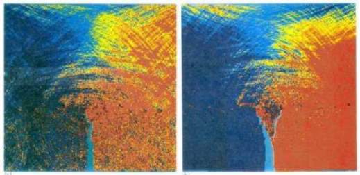
Fig. 3.2: Molecular dynamics simulation of crack propagation using multiscale modelling (Source: Google)

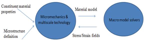
Fig. 3.3: Multiscale modelling in a nutshell (Source: Google)

3.5 Plasticity Models

In essence, plasticity theory, and therefore models based upon it, has the following main ingredients, a yield surface, a flow rule and a hardening function or plastic evolution equation. Additionally, for the small strain case, plasticity models assume an additive decomposition or split of the total strain into the elastic strain and the plastic strain respectively and a constitutive relationship for the elastic part. The yield surface, defined by a yield function, initially bounds the elastic domain in the stress space and its evolution (i.e. the way it expands or contracts in the stress or strain space) is controlled by the hardening function. Finally, the flow rule governs the evolution of the plastic strain. The yield criterion (Iulia C. Mihai ,2012) is generally expressed as:

F(σ, K) ≤ 0                                  Eq.(3.3)

where σ is the stress tensor and K denotes the hardening variable. In general, yield surfaces have been proposed based upon biaxial and/or triaxial failure envelopes for concrete obtained experimentally.

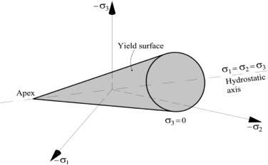
Fig. 3.4: Yield surface for Drucker-Prager plasticity model (Source: Google)

The failure surface has an open shape, as indicated directly by experiments. In contrast, observations of the non-linear behaviour of concrete show that the initial yield surface should be “capped” to account for the plastic deformations which take place under hydrostatic compression.

3.6 Damage Models

The roots of damage theory date back to 1958 with the definition of a scalar damage variable by Kachanov, although Hult was the first to introduce the term “continuum damage mechanics” in 1972. Formulations based on continuum damage mechanics describe the progressive degradation of stiffness resulting from the propagation of microcracks. The degree of degradation is characterized by damage parameters that can be scalars, a family of vectors or in the most general case a fourth-order tensor. Somewhat similar to plasticity theory, damage mechanics theory employs a damage function that controls the initiation of damage and evolution functions that govern the manner in which the damage function progresses with the damage parameter. These equations are generally written in terms of strains, stresses or energy based variables derived within a thermodynamic framework. The fundamental concepts of damage mechanics are best illustrated by a simple isotropic damage model which employs a simplifying assumption that the degradation of stiffness is isotropic. With an additional assumption that the Poisson’s ratio remains unaffected, damage can be characterized by a single scalar parameter.

σ = (1 – w) D_el: ε         Eq. (3.4)

where ‘:’ denotes tensor contraction. σ and ε represent the macroscopic stress and strain tensor respectively, D_el is the elasticity tensor of the undamaged material and w is the damage parameter generally defined such that it grows from 0 for an undamaged state to 1 for a fully damaged state.

Formulations of constitutive models for concrete that combine plasticity and damage theory have been proposed based on the argument that plasticity or damage theories employed on their own were not sufficient to capture key characteristics of the overall behaviour. But plasticity theory is not able to address properly the stiffness degradation due to micro cracking whereas models based on continuum damage theory alone cannot capture other important facets of concrete behaviour such as permanent deformations and inelastic volumetric expansion in compression.

Damage in concrete, however, is not an isotropic process and models based on the isotropic damage assumption in general experience a number of deficiencies; in particular they are unable to capture the volumetric expansion (dilatancy) observed in uniaxial compression experimental tests and for large tensile strains applied in one direction the stiffness is completely lost in the loading direction and unrealistically reduced in lateral directions. In order to overcome these drawbacks, formulations have been explored and proposed that take into account the damage induced anisotropy. These anisotropic formulations however have a higher level of complexity as they usually employ second or even fourth-order tensors to characterize damage and they exhibit serious convergence problems when implemented in finite element codes. These drawbacks often cause the simplified although unrealistic assumption of isotropic damage to be preferred and employed over the anisotropic damage assumption. The reduction of stiffness and strength of concrete comes as a direct result of the onset and propagation of microcracking.

Nevertheless, stress states do exist for which this effect diminishes or can disappear altogether. For instance when a previously open crack, which contributed to the stiffness reduction, is subsequently subjected to compressive stresses normal to the crack plane, it closes and the crack faces regain contact. The compressive stresses can thus be transferred across the crack plane although the damage state does not change (the damage parameter does not reduce). These phenomena are referred to as unilateral or crack closure effects, damage deactivation or stiffness recovery.

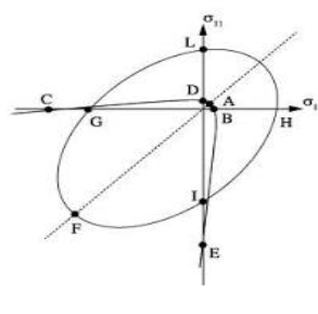
Fig. 3.5: Linear elastic domain in the principal stress plane of damage model (Source: Google)

3.7 Plastic-damage models

Moreover, it was suggested based on observations of the behaviour of concrete in tension and compression cyclic tests, that on one hand the tensile behaviour with an approximately secant unloading path is better reproduced by damage theory and on the other hand behaviour in compression, which follows a relatively elastic unloading path, is captured better by pure plasticity. This model represents the inelastic behaviour of concrete by using the concepts of isotropic damaged elasticity in combination with isotropic tensile and compressive plasticity. The model describes the irreversible damage in concrete due to the fracturing process by a combination of non-associated multi-hardening plasticity and scalar damaged elasticity. In general, plastic-damage models combine isotropic hardening with either isotropic damage or anisotropic damage.

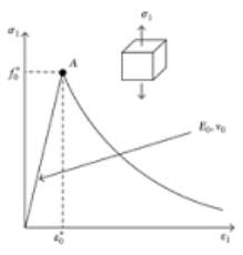
Fig. 3.6: Coupled plastic damage model for concrete (Source: Google)

3.8 Micromechanical models

A micromechanical constitutive model for concrete is proposed in which microcrack initiation, in the interfacial transition zone between aggregate particles and cement matrix, is governed by an exterior-point Eshelby solution. It predominantly involves numerical modelling of restricted volumes of material. The model assumes a two-phase elastic composite, derived from an Eshelby solution and the Mori-Tanaka homogenization method, to which circular micro cracks are added. A multi-component rough crack contact model is employed to simulate normal and shear behaviour of rough micro crack surfaces. It is shown, based on numerical predictions of uniaxial, biaxial and triaxial behaviour that the model captures key characteristics of concrete behaviour. An important aspect of the approach taken of this micromechanical modelling is its adherence to a mechanistic modelling philosophy. In this regard the model is distinctly more rigorously mechanistic than its more phenomenological predecessors.

Phenomenological models generally employ theories based on plasticity and /or damage mechanics in order to simulate the macroscopic behaviour and their formulation often makes use of functions obtained by fitting experimental data (e.g. uniaxial tension and compression curves, strength envelopes). On the other hand micromechanical models aim to relate the microstructure of concrete, and the physical mechanisms that govern its evolution, to the macroscopic behaviour observed in experiments.

Generally, the aim with micromechanical models is to capture the macroscopic mechanical behaviour observed in experiments by simulating simple physical mechanisms at micro and mesoscale. This is in contrast with the phenomenological macroscopic models for which uniaxial compression, uniaxial tension functions and strength envelope equations are generally prescribed directly. The mechanistic micromechanical models combine individual mechanistic components to predict a response which is not pre-prescribed. This means that the prediction of behaviour as apparently simple as the uniaxial compressive response of concrete, with the near peak associated dilatancy becomes a significant challenge. This challenge is, however, worth addressing because all present macroscopic models have shortcomings.

3.9 Microplane models

A complex material model causes ample difficulties for identifying respective material parameters and also for interpreting the physical meaning of the components of the damage tensor. An efficient and better approach to describe this anisotropic material response in a natural and simple way is delineated by the microplane theory. Microplane material model clearly describes the material behaviour on a mesoscopic scale.

The basic aspect of the microplane concept is to formulate the constitutive equations between single scalar and vector valued stress-strain components on individual microplanes. Thus the microplane parameters obtain a physical meaning and interpretation(Michael Leukart and Ekkehard Ramm, 2006).

The characterization of the material behaviour on different planes was initially suggested by Mohr in 1900 and was first applied to metals by Taylor in 1938. Efforts and works by Bazant, Oh and Gambarova for two decades transferred this idea to a continuum damage description. A successful realization of microplane modelling in the context of quasi-brittle materials like concrete has been progressively advanced by Bazant and Prat (1988), Carol et.al (1992), Bazant and Planas (1998) and Bazant et.al (2000).

Bazant and Ozbolt developed a nonlocal version of the microplane model in 1992 to avoid mesh dependent solutions in the stain softening region. Jirasek and Carol et.al in 2000 established a thermodynamically consistent framework for microplane models in a way that it satisfies the second law of thermodynamics.

For a certain class of materials, due to the definition of pure volumetric and deviatoric components on the mesoscale, it can be transferred to the macroscale in an analogous manner. One specialized benefit of the microplane formulation is its close relation to macroscopic models. These microplane models are based on the formulation of phenomenological constitutive laws, with parameters identified by experiments through inverse identification, without a direct physical interpretation of the constitutive behaviour on the individual microplanes.

Microplane model makes it possible to clearly describe the general anisotropic responses of a wide class of materials. The basic requirement of the microplane model is to capture at least the material responses of classical macroscopic damage and plasticity material formulations on the macroscopic level. Brocca, Bazant and Kuhl et.al in 2000, pioneered efforts in the field of microplane plasticity. They have shown to express microplane plasticity parameters in terms of macroscopic quantities such as the tensile strength and compressive strength.

The main purpose of the microplane approach is to describe material behavior that cannot be easily determined by conventional macroscopic tensorial constitutive models (Bazant and Caner, 2005). The important feature of this model is a split of the local microplane strains and stresses. It allows one to resort to simplified stress-strain relationship or in certain cases even unidirectional constitutive laws.

From the macroscopic viewpoint, it is recommended to restrict the microplane concept to the pure volumetric-deviatoric split which is a constraint subset of the most often applied volumetric-deviatoric-tangential split. Volumetric-deviatoric split has the particular advantage that typical macroscopic responses are directly reflected on the mesoscale.

It was also shown that in certain cases the present version of a microplane formulation is closely related to well-known macroscopic models although being much more general than those macroscopic formulations. This close relation is exploited to derive physically sound microplane constitutive laws. Identification and interpretation of the microplane constitutive laws was done by the comparison of the microplane formulation to a well-known macroscopic one-parameter damage model and the constitutive formulations are embedded in a thermodynamically consistent framework.

CHAPTER 4

VALIDATION

4.1 NUMERICAL ANALYSIS OF A SIMPLY SUPPORTED RC BEAMUSING ANSYS

Dynamic platform: ANSYS Mechanical APDL 15

Validation is done based on the paper “Flexural Behaviour of RCC Beams” by S Tejaswi, 2015.

Size of the beam: 1200 mm x 200 mm x100 mm

Concrete: M30

Steel: Fe415

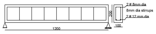
Fig. 4.1: Beam detailing (Dimensions in mm)

4.1.1 ANSYS Software

ANSYS is a finite element analysis (FEA) code widely used in the computer-aided engineering (CAE) field. ANSYS software allows engineers to construct computer models of structures, machine components or systems; apply operating loads and other design criteria; and study physical responses, such as stress levels, temperature distributions, pressure, etc. It permits an evaluation of a design without having to build and destroy multiple prototypes in testing.

The ANSYS computer program is a general purpose Finite Element Modelling Package for numerically solving a variety of engineering problems. These problems include static and dynamic structural analysis (both linear and non-linear), steady state and transient heat transfer problems, mode-frequency and buckling analyses, acoustic and electromagnetic problems and various types of field and coupled-field applications. The program contains many special features which allow nonlinearities to be included in the solution such as plasticity, large strain, hyper elasticity, creep, swelling, large deflections, contact, stress stiffening, temperature dependency, material anisotropy and radiation.

All users, from designers to advanced experts, have benefit from ANSYS structural analysis software. The reliability of result achieved through the wide variety of material model available, the quality of the element library, performance permanency of solution algorithms, and ability to model from every single parts to complex assemblies.

The ANSYS finite element program (ANSYS 15), operating on a window x64 system, was used in this study. Each program, however, has its own nomenclature and specialized elements and analysis procedure that need to be used properly.

4.1.2 Element types used for analysis

(i) Concrete

A Solid65 element was used to model the concrete. This element has eight nodes with three degrees of freedom at each node translations in the nodal x, y, and z directions.Solid65 is used for the 3-D modelling of solids with or without reinforcing bars (rebar). The solid is capable of cracking in tension and crushing in compression. The concrete element is similar to a 3-D structural solid but with the addition of special cracking and crushing capabilities.

The most important aspect of this element is the treatment of nonlinear material properties. The concrete is capable of cracking (in three orthogonal directions), crushing, plastic deformation, and creep. The rebar are capable of tension and compression, but not shear. They are also capable of plastic deformation and creep. The solid capability of the element may be used to model the concrete while the rebar capability is available for modelling reinforcement behaviour. Other cases for which the element is also applicable would be reinforced composites (such as fiber glass), and geological materials (such as rock).  The geometry of element solid 65 is  shown in Fig.3.6.

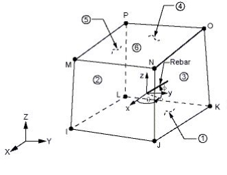
Fig. 4.2: Solid 65 element

(ii) Steel Reinforcement

A Link180 element was used to model steel reinforcement. This element is a 3D spar element and it has two nodes with three degrees of freedom translations in the nodal x, y, and z directions. This element is capable of plastic deformation. Link 180 useful for variety of engineering applications. The element can be used to model trusses, sagging cables, links, springs, and so on. The element is a uniaxial tension or compression element. Tension-only (cable) and compression-only (gap) options are supported. As in a pin-jointed structure, no bending of the element is considered. Plasticity, creep, rotation, large deflection, and large strain capabilities are included. The element is capability of plastic deformation.

Fig. 4.3: Link 180 element

LINK180 includes stress-stiffness terms in any analysis that includes large-deflection effects. Elasticity, isotropic hardening plasticity, kinematic hardening plasticity, Hill anisotropic plasticity, and creep are supported. To simulate the tension or compression only options, a nonlinear iterative solution approach is necessary; therefore, large-deflection effects must be activated prior to the solution phase of the analysis. The geometry of this element type is shown in fig.4.3.

4.1.3 Real Constants used for analysis

Real Constant Set 1 was used for the Solid 65 element. It requires real constants for rebar assuming a smeared model. Values can be entered for Material Number, Volume Ratio, and Orientation Angles. The material number refers to the type of material for the reinforcement. The volume ratio refers to the ratio of steel to concrete in the element. The reinforcement has uniaxial stiffness and the directional orientations were defined by the user. In the present study the beam was modeled using discrete reinforcement. Therefore, a value of zero was entered for all real constants, which turned the smeared reinforcement capability of the Solid65 element of Real Constant Sets 2 and 3 were defined for the Link180 element. Values for cross-sectional area and initial strain were entered. Cross-sectional area in set 2 refers to the reinforcement of two numbers of 10mm diameter bars and in set 3 refers to the 8 mm diameter two legged stirrups.

4.1.4 Engineering data used in analysis

Table 4.1: Engineering data for steel

Linear Isotropic
Youngs Modulus	200000 MPa
Poissons ratio	0.3
Bilinear Isotropic
Yield Stress	415 MPa
Tangent Modulus	20 Mpa

Table 4.2: Engineering data for concrete

Linear Isotropic
Youngs Modulus	27386 MPa
Poissons ratio	0.2

ANSYS has its own non-linear material model for concrete. Its reinforced concrete model consists of a material model to predict the failure of brittle materials, applied to a three-dimensional solid element in which reinforcing bars may be included. The material is capable of cracking in tension and crushing in compression. It can also undergo plastic deformation and creep.

4.1.5 Loads and Boundary Conditions

Displacement boundary conditions were needed to constraint the model to get a unique solution. To ensure that the model acts the same way as the experimental beam boundary conditions need to be applied at points of symmetry, and where the supports and loading exist.  It was modeled with pinned support at one end and roller at the other end. Nodes on the plate were given constraint in all directions, applied as constant values of zero. The loading and boundary conditions of the beam are shown in Fig.4.4.

4.1.6 Numerical modelling

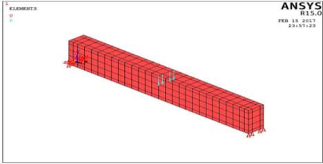
Fig.4.4: Loading diagram with support conditions

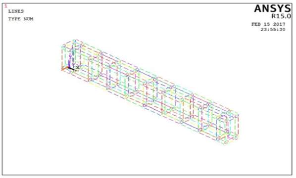
Fig. 4.5: Reinforced model of the beam

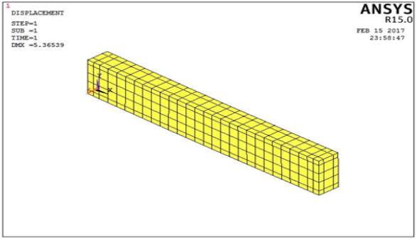
Fig. 4.6: Deflection Diagram

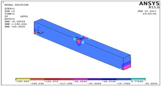
Fig. 4.7: Stress Diagram

4.1.7 Results

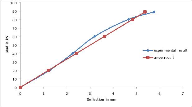
Fig. 4.8: Load – Deflection Graph

Table 4.3: Deflection at ultimate load

Ultimate Load (kN)	Deflection in mm (experiment)	Deflection in mm (software)	% Variation
88.8	5.75	5.36	7.27

By modelling and analyzing in ANSYS Mechanical APDL 15, deflections obtained for different loads until ultimate load has been plotted. Table 4.3 shows the comparison between deflections obtained from finite element software with that of experiment.

 

 

 

 

 

 

 

 

 

 

CHAPTER 5

NUMERICAL ANALYSIS OF A SIMPLY SUPPORTED RC BEAMUSING MICROPLANE MODELLING

 

5.1 MICROPLANE MODELLING

 

5.1.1 General

The microplane model was developed by Bazant et.al in 1980. The first generalized microplane model employed an idea, initially proposed by Taylor (1938) and subsequently applied by Batdorf and Budianski (1949) in a constitutive model for polycrystalline metals.

According to Taylor (1938) the stress strain relationship of a material can be defined in an independent manner on planes of various orientations called microplanes, by assuming either a static constraint (i.e. the stresses on a microplane are the resolved components of the macroscopic stress) or a kinematic constraint (i.e. the strains on a microplane are the resolved components of the microscopic strain tensor). The kinematic constraint was adopted by Bazant and Prat (1988) since it enabled a stable response during strain softening.

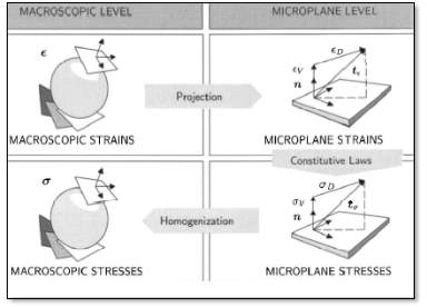
Fig. 5.1: Microplane theory based on the kinematic constraint and V-D split (Michael et.al, 2006)

The essential feature of this material formulation is a split of the local microplane strains and stresses allowing one to resort to simplified or in certain cases even unidirectional constitutive laws. The main attraction of the microplane concept is that an initial or evolving anisotropic material behaviour can be described in a natural and simple way. Motivated from a macroscopic viewpoint, it is advocated to restrict the microplane concept to the pure volumetric-deviatoric split, as a constraint subset of the most often applied volumetric-deviatoric-tangential split. This variant has the particular advantage that typical macroscopic responses are directly reflected on the mesoscale.

The microplane theory is shortly summarized in a schematic form in Fig. 5.1. The three main steps of the microplane model are illustrated. The first step is the projection part. Here a kinematic constraint is applied in order to relate the macroscopic strain tensor to their microplane counterparts. The kinematic constraint assumes that the microplane strains are equivalent to the projected macroscopic strain tensor, opposite to a static constraint, where the stresses are projected.

The microplane strains can be derived as projections of the overall strain tensor ε, which corresponds to the symmetric part of the displacement gradient in the geometrically linear case. The second step describes the definition of constitutive laws on the microplane level. These constitutive equations are formulated between single stress and strain components on individual microplanes.

The methodology of the two traditional splits, the so-called normal-tangential and the volumetric-deviatoric-tangential can be gleaned in Bazant and Prat (1988) and Kuhl and Ramm (2000). This split is known from classical continuum mechanics for the macroscopic strain and stress tensor for materials with a distinct volumetric-deviatoric constitutive behaviour. The last step of microplane modelling relates to the homogenization process on the material point level to derive the overall response. This homogenization process is based on the principle of energy equivalence.

In former microplane formulations, the overall response was derived through a homogenization process based on the principle of virtual work (PVW), which postulates that the macroscopic virtual work of a material point is equal to the virtual work on all microplanes of this material point. But some microplane models based on the V-D-T split or V-D split and derived from the PVW may lead to negative energy dissipation. In other words it is possible to generate energy under certain loading conditions and thus the second law of thermodynamic is violated.

This concept of energy equivalence is based on the fundamental assumption, that a microscopic free energy on the microplane level Ψ^mic exists and the integral of Ψ^mic over all microplanes is equivalent to a macroscopic Helmholtz free energy density Ψ^mac:

Ψ^mac =

34π∫ΩΨmic dΩ                                                     Eq.(5.1)

For the sake of a consistent notation it has been stick to the notion “microscopic” although the material model is rather mesoscopic than a truly micromechanical description.

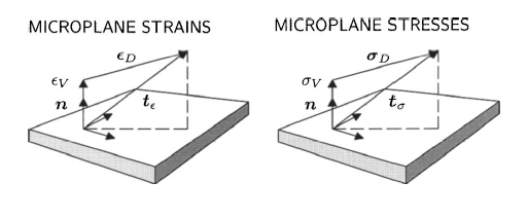
Fig. 5.2: Model with volumetric and deviatoric microplane components (Michael et.al, 2006)

The basic hypothesis of the kinematic constraint is that the strain vector t_ε on each microplane is the normal projection of the macroscopic strain tensor ε,

t _{ε =} ε. n                                                  Eq.(5.2)

This strain vector on a microplane will be the starting point for the characterization of different microplane formulations. The choice of relevant strain components is a very crucial point in defining the appropriate microplane model. Three different types of splits can be distinguished (Leukart and Ramm, 2002). The V-D split describes an effective approach for the modelling of materials with a distinct volumetric-deviatoric constitutive behaviour. This split has the particular advantage that macroscopic responses are directly reflected on the microplane level and is therefore preferred. The motivation for the V-D split is that for many materials the volumetric and deviatoric behaviour is completely different, not only on the macroscopic level but also on the microplane level. The kinematic basis is the decomposition of the macroscopic strain tensor into a volumetric and deviatoric part. For the sake of transparency, V-D split is derived from the additive decomposition of the strain tensor and project each part of the strain tensor, the volumetric and the deviatoric one, onto the microplanes. This leads to a clear decomposition of the strain vector into a volumetric and deviatoric component, illustrated in Fig. 5.2.

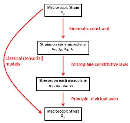
Fig. 5.3: Microplane formulation (Giovanni Di Luzio, 2016)

Microplane theory is summarized in three primary steps.

1.                Apply a kinematic constraint to relate the macroscopic strain tensors to their microplane counterparts.
2.                Define the constitutive laws on the microplane levels, where unidirectional constitutive equations (such as stress and strain components) are applied on each microplane
3.                Relate the homogenization process on the material point level to derive the overall material response. (Homogenization is based on the principle of energy equivalence.)

As mentioned before the microplane material model formulation is based on the assumption that microscopic free energy Ψ^mic on the microplane level exists and that the integral of Ψ^mic over all microplanes is equivalent to a macroscopic free Helmholtz energy Ψ^mac (Eq. 5.1).The factor

34π  results from the integration of the sphere of unit radius with respect to the area Ω.

The strains and stresses at microplanes are additively decomposed into volumetric and deviatoric parts, respectively, based on the volumetric-deviatoric (V-D) split.

The strain split is expressed as:

ε = ε_D +ε_V 1                                                            Eq.(5.3)

The scalar microplane volumetric strain ε_v results from:

ε_V = V : ε                                                               Eq.(5.4)

where V =

13 1 is the second-order volumetric projection tensor and 1 the second-order identity tensor.

The deviatoric microplane strain vector ε_D is calculated as:

ε_D= Dev : ε                                                            Eq. (5.5)

where,

Dev = n.π –

13n.1 x 1= n.π ^dev                                               Eq. (5.6)

and “π” is the fourth-order identity tensor and the vector “n” describes the normal on the microsphere (microplane).The macroscopic strain ε is expressed as:

ε =

34π∫(Vεv +Dev^T. ε_D) dΩ                                       Eq. (5.7)

The stresses can then be derived as

σ =

34π∫(Vσ_v+

Dev^T_.σ_D) dΩ                                          Eq.(5.8)

whereσ_v andσ_D are the scalar volumetric stress and the deviatoric stress tensor on the microsphere,

σ = V :σ                                                         Eq. (5.9)

and

σ_D = Dev : σ                                                    Eq. (5.10)

Assume isotropic elasticity:

σ_v= K^micε_v                                                                                   Eq. (5.11)

σ_v = G^micε_D                                                                                 Eq. (5.12)

where K^mic and G^mic are microplane elasticity parameters and can be interpreted as a sort of microplane bulk and shear modulus.The integrals of the macroscopic strain equation and the derived stresses equation are solved via numerical integration:

σ =

34π 

∫Ω.  ^mic

dΩ                                                                         Eq. (5.13)

where wⁱ is the weight factor.

5.1.2 Discretization

Discretization is the transfer from the microsphere to microplanes which describe the approximate form of the sphere. Forty-two microplanes are used for the numerical integration. Due to the symmetry of the microplanes (where every other plane has the same normal direction), 21 microplanes are considered. Fig.5.4 illustrates the discretization process.

To account for material degradation and damage, the microscopic free-energy function is modified to include a damage parameter, yielding:

Ψ^mic (ε_v, ε_D, d^mic) = (1- d^mic) Ψ^mic (ε_v,ε_D)                       Eq. (5.14)

The damage parameter d^mic is the normalized damage variable { 0 ≤ d^mic ≤ 1}.

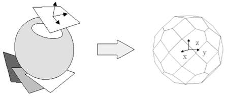
Fig. 5.4: Sphere Discretization by 42 Microplanes(Michael et.al, 2006)

The stresses are derived by:

σ =

34π∫(Vεv +Dev^T. σ _D) dΩ                                         Eq. (5.15)

where

σ _D (ε_D, d^mic) = (1- d^mic ) G^micε_D                                                          Eq. (5.16)

σ_V (ε_V, d^mic) = (1- d^mic ) K^micε_V                                                          Eq. (5.17)

The damage status of a material is described by the equivalent-strain-based damage function,

φ = φ^mic(η^mic) – d^mic   ≤   0                                             Eq. (5.18)

where η^mic is the equivalent strain energy, which characterizes the damage evolution law and is defined as:

η^mic = K₀ I₁ + ( K₁²I₁² + K₂J₂)^1/2                                                                 Eq. (5.19)

where I₁ is the first invariant of the strain tensor ε, J₂ is the second invariant of the deviatoric part of the strain tensor ε, and k₀, k₁, and k₂ are material parameters that characterize the form of damage function. The equivalent strain function implies the Mises-Hencky-Huber criterion for k₀ = k₁= 0, and k₂ = 1, and the Drucker-Prager-criterion for k₀ > 0, k₁ = 0, and k₂ = 1.

The damage evolution is modeled by the following function:

d^mic= 1 –

γ micηmic[ 1- α^mic + α^mic.exp (β^mic(

γ mic–

ηmic) )) ]                     Eq. (5.20)

where α^mic defines the maximal degradation, β^mic determines the rate of damage evolution, and

γ mic characterizes the equivalent strain energy on which the material damaging starts (damage starting boundary).The material parameters in the model are: E, ν, k0, k1, k2,α^mic,

γ^mic, and βmic.

Table 5.1: Material constants of microplane model

C1	k0	Damage function constant
C2	k1	Damage function constant
C3	k2	Damage function constant
C4	ϒmic	Critical equivalent strain energy density
C5	αmic	Maximum damage parameter
C6	βmic	Scale for rate of damage

k =

fcft                                                               Eq. (5.21)
k₀ =

k-12k (1-2v)                                                Eq. (5.22)
k₁=k₀                                                             Eq. (5.23)
k₂=

3(1+v)k(1-v)                                                   Eq. (5.24)
where ,

fc – compressive strength

ft – tensile strength

v – Poisson’s ratio

 

5.1.3 Advantages of microplane model

1. The constitutive law is written in terms of vectors rather than tensors.

2. The inelastic physical phenomena associated with surfaces, such as slip, friction, tensile cracking, or lateral confinement on a given plane or its spreading, can be characterized directly in terms of the stress and strain on the surface on which they take place.

3. In computational practice, macroscopic tensorial plastic-damage models with only one or two loading surfaces are generally used. For such models, most materials appear to exhibit large apparent deviations from the normality rule for the plastic strain increments.

4. Unlike the classical plasticity models used in computational practice, the microplane model captures the so-called vertex effect.

5. Extension to strain softening requires making the yield surfaces dependent on the strains.

6. The interaction of microplanes due to the kinematic constraint suffices to provide all the main cross effects on the macro level, such as the pressure sensitivity of inelastic shear strain and the dilatancy.

7. A vast number of combinations of loading or unloading on various microplanes is possible, and some microplanes unload even for monotonic loading on the macroscale.

8. The microplane model can naturally model fatigue, as well as hysteresis during cyclic loading.

9. With the microplane approach, anisotropic materials are not appreciably more difficult to model than isotropic materials.

10. The philosophies of the microplane approach and finite elements blend well.

 

 

 

 

5.2 NUMERICAL MODELLING AND USE OF MICROPLANE MODEL IN A SIMPLY SUPPORTED RC BEAM

An RC beam as per “Effect of manufactured sand as fine aggregate on the strength, durability and structural properties of concrete” by P.M Shanmughavadivu, 2013 has been modelled and microplane model has been used in it.

Concrete: M30

Steel:  Fe415

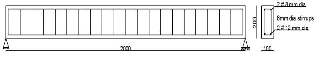
Fig. 5.5: Beam detailing (Dimensions in mm)

5.2.1 Numerical modelling of a simply supported RC beam with microplane

 

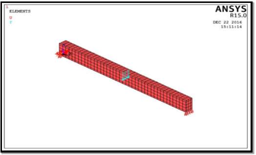
Fig. 5.6: Loading diagram with support conditions

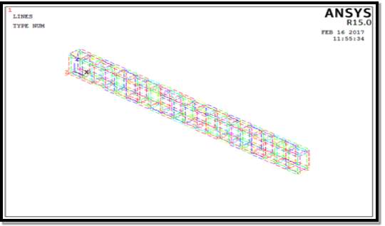
Fig. 5.7: Reinforcement model of the beam

Using this reference beam, a number of models and analysis has been done in ANSYS Mechanical APDL 15 for different combinations of material models like:

1. Concrete (Linear) & Steel (Linear)
2. Concrete (Linear, multi linear) & Steel (Linear)
3. Concrete (Linear, multi linear ) & Steel(linear, bilinear)
4. Case 1: Concrete (microplane)
5. Case 2: Steel (microplane)
6. Case 3: Concrete (microplane) & Steel (microplane)
7. Case 4: Concrete (microplane, multi linear) & Steel (microplane, bilinear)

 

 

 

 

 

5.2.2 Results and Discussion

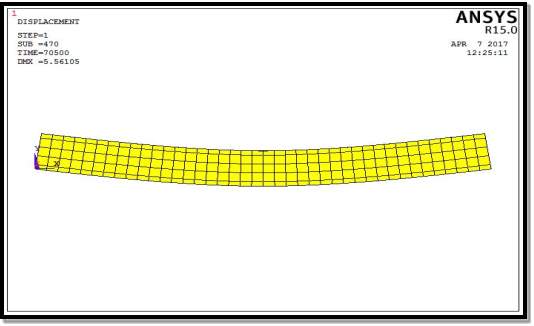
Fig. 5.8: Deflection Diagram (Concrete (Linear) & Steel (Linear))

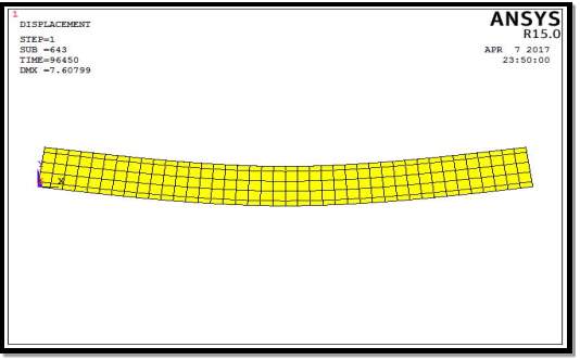
Fig. 5.9: Deflection Diagram ((Concrete (Linear, multi linear) & Steel (Linear))

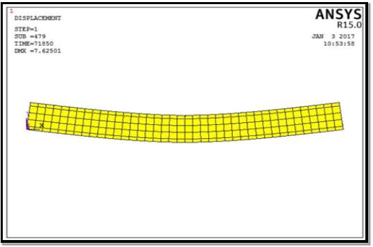
Fig. 5.10: Deflection Diagram (Concrete (Linear, multi linear) & Steel (linear, bilinear))

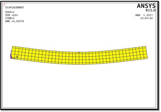
Fig. 5.11: Deflection Diagram (. Case 1: Concrete (microplane))

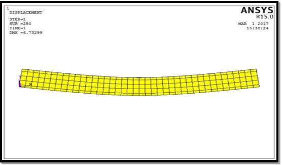
Fig. 5.12: Deflection Diagram (Case 2: Steel (microplane))

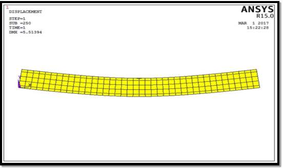
Fig.5.13: Deflection Diagram (Case 3: Concrete (microplane) & Steel (microplane))

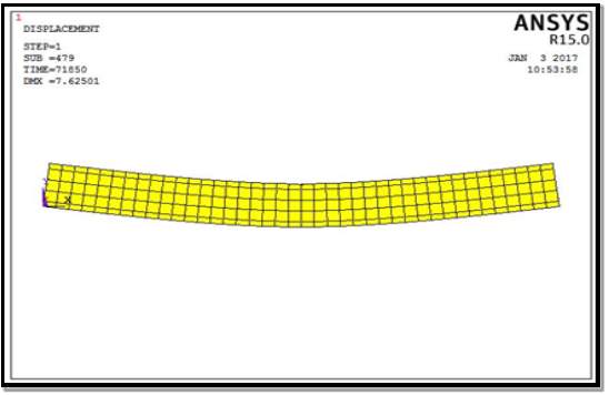
Fig. 5.14: Deflection Diagram (Case 4: Concrete (microplane, multi linear) & Steel (microplane, bilinear)

Using all these combinations, beams has been modelled, analyzed and the load – deflection graph has been plotted all these 7combinations. From the load deflection graph, we can see that finite element program using microplane model is giving comparable as well as better results with that of experiment than simply using material models available in the software (Fig.5.15).

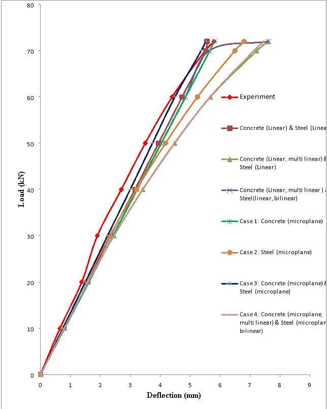
Fig. 5.15: Load deflection graph for different combinations of material models

Table 5.2: Ultimate load and deflection for different combinations

Combination of material models	Deflection at ultimate loads (mm)
1.Concrete (Linear) & Steel (Linear)	5.56
2.Concrete (Linear, multi linear) & Steel (Linear)	7.6
3.Concrete (Linear, multi linear ) & Steel(linear, bilinear)	7.62
4.Case 1: Concrete (microplane)	5.808
5.Case 2: Steel (microplane)	6.73
6.Case 3: Concrete (microplane) & Steel (microplane)	5.51
7.Case 4: Concrete (microplane, multi linear) & Steel (microplane, bilinear)	7.74

 

Table 5.2 shows the deflections at ultimate loads for different cases as well as the experimental deflection. From this, once again we can see that, beams modelled using microplane model is giving better as well as comparable results with that of using finite element software alone. And the analysis with microplane model used only for concrete is giving the closest result to that of experiment towards the ultimate load since deflection at ultimate load from experiment) = 5.8 mm (P.M Shanmughavadivu,2013) , even though combination with microplane model used for both concrete and steel is giving closest results in the initial region (Fig.5.15). Microplane model when used for both concrete and steel obtained an average variation of only 9.94% with experiment. Percentage variation of deflection at ultimate load, when microplane model used for concrete is only 0.14%. Therefore, for further studies, microplane model has been used only for concrete

 

 

5.3 PARAMETRIC STUDY AND CRACK SIMULATION OF RC DEEP BEAM USING MICROPLANE MODEL

Deep beams has been modelled using microplane model as per “Experimental and Analytical Study on Reinforced Concrete Deep Beam” by Prof. S. S. Patil et.al (2013).

Dynamic platform: ANSYS Workbench 15 & ANSYS Mechanical APDL 15

Support condition: Hinged at both ends

Concrete: M30

Steel: Fe415

5.3.1 Details of Beams used for Parametric Study

The parametric study is carried out to study the influence of various parameters, namely, span to depth ratio and percentage of steel on the shear strength of concrete deep beams. The magnitudes of span to depth ratio considered were 1.5, 1.6 and 1.71(or shear span to depth ratio 0.5, 0.53 and 0.57) and the percentage of steel varied from 0.5, 1, 1.5 to 2 percent.

• Effective span, L = 600 mm
• Cross section of Beam # 1 – 150 mm x 350 mm (L/D ratio – 1.71)
• Cross section of Beam # 2 – 150 mm x 375 mm (L/D ratio – 1.6)
• Cross section of Beam # 3 – 150 mm x 400 mm (L/D ratio – 1.5)

5.3.2 Stress strain relationship for concrete

The uniaxial stress-strain relationship for concrete in compression was provided while modelling in ANSYS. For concrete, stress-strain curve has been plotted and non-linear properties were provided based on Mac Gregor Equation.

Stress,       f =

Ec x ℇ1+(ℇ/ℇ0)2                                                        (Eq.5. 25)

where,

E_c=

5000√fck                                                                 (Eq.5. 26)

ℇ

₀ 

=2fckEc                                                           (Eq.5. 27)

f_c = 0.8 f_ck                                                                    (Eq.5. 28)

5.3.3 Numerical analysis of deep beams

 

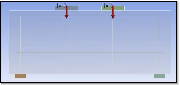
Fig.5.16: Deep beam model with loading (Beam #1)

5.3.4 Results and Discussion

1. Beam # 1

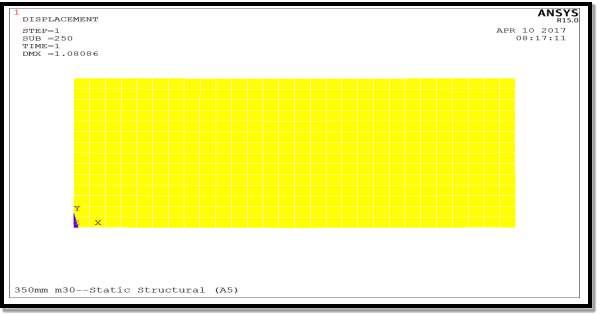
Fig. 5.17: Deflection diagram

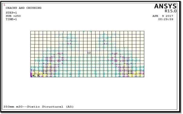
Fig. 5.18: Crack pattern

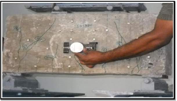
Fig. 5.19: Crack pattern from experiment (S.S Patil,2013)

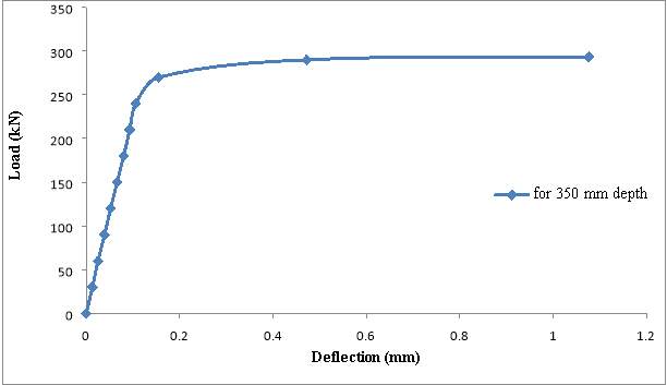
Fig. 5.20: Load deflection graph

2. Beam # 2

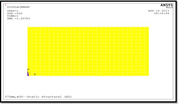
Fig. 5.21: Deflection diagram

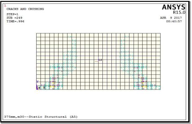
Fig. 5.22: Crack pattern

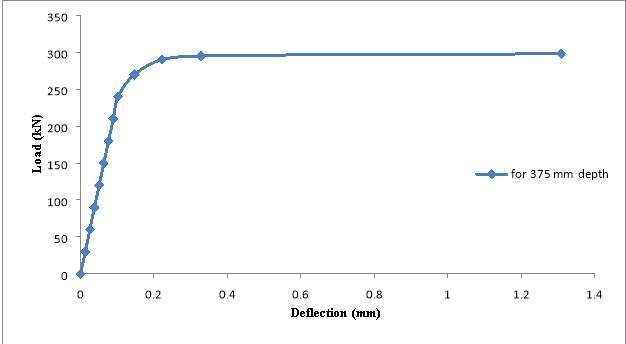
Fig. 5.23: Load deflection graph

3. Beam # 3

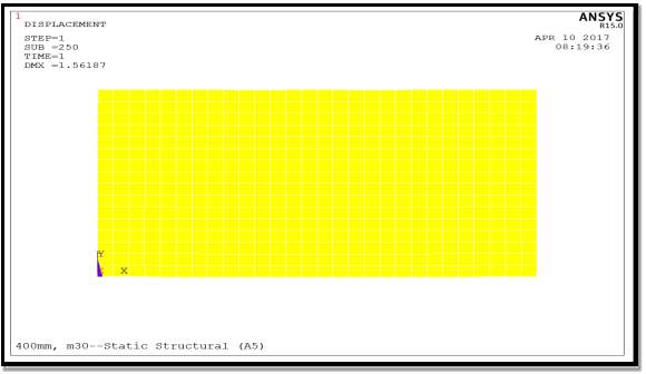
Fig. 5.24: Deflection diagram

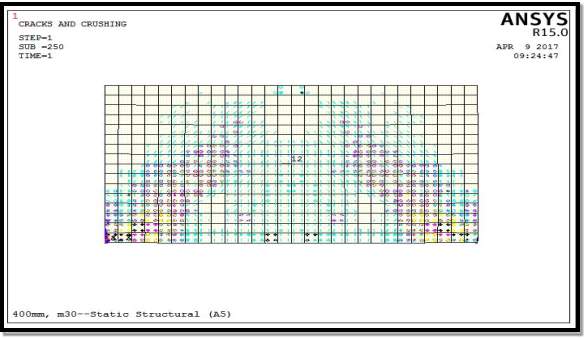
Fig. 5.25: Crack pattern

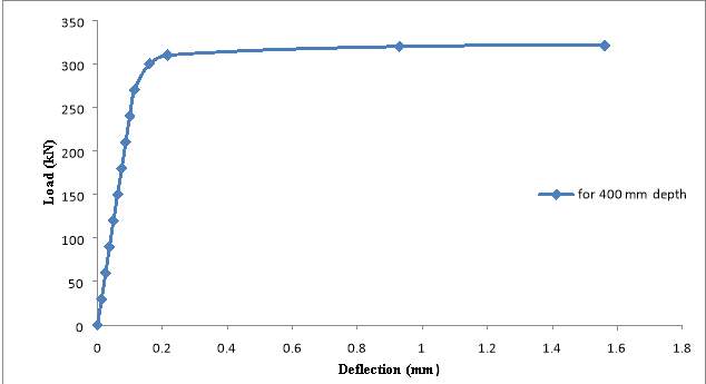
Fig. 5.26: Load deflection graph

Table 5.3: Analytical results for beams

L/D Ratio	Ultimate load (kN)	Deflection (mm)	Load at first crack (S.S Patil,2013) (kN)	Load at first crack (kN)	Load at second crack (kN)	Load at third crack (kN)
1.5	321	1.56	213.1	178.6	291	313
1.6	298	1.305	183.3	170	263	285
1.71	293	1.0768	168.3	166.8	260	282

From Table 5.3, we can see that,

• As L/D ratio increased from 1.5 to 1.71, load carrying capacity decreased by 9.5%.
• As L/D ratio increased from 1.5 to 1.71, load at first crack decreased by 7.07%.
• As L/D ratio increased from 1.5 to 1.71, load at second crack decreased by 11.9%.
• As L/D ratio increased from 1.5 to 1.71, load at third crack decreased by 10.9%.

Table 5.4: Comparison of shear strength obtained using microplane model with that of experiment

L/D Ratio	Shear strength (Experiment- S.S Patil,2013)	Shear Strength (Microplane Model)	% Variation
1.5	160	160.5	0.31
1.6	150	149	0.67
1.7	145	146	0.69

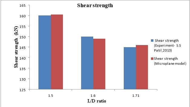
Fig. 5.27: Graphical representation of shear strength obtained for l/D ratios 1.5, 1.6, 1.71 with that of experiment

From Table 5.4, the average percentage variation of shear strength from that of experiment is only 0.55%. Therefore, further parametric study on shear strength was conducted using microplane model for different longitudinal reinforcement ratios, 0.5, 1, 1.5 and 2%. For the parametric study, 16 deep beams were modelled using microplane. The result for parametric study has been tabulated as shown in Table 5.5.

Table 5.5: Shear strength for different L/D ratios and longitudinal reinforcement ratios

L/D	SHEAR STRENGTH (kN)
	Pt = 0.5%	Pt = 1%	Pt = 1.5%	Pt = 2%
1.5	163.5	174	177	182.5
1.6	155	165	170	175
1.71	148	156	163	168

 

 

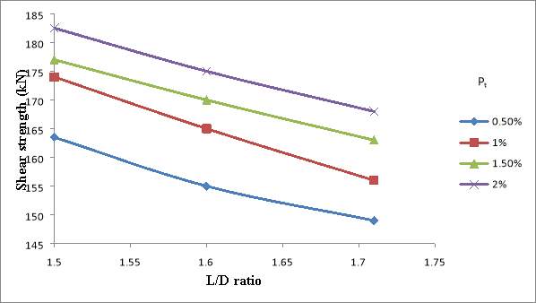
Fig. 5.28: Graphical representation of the effect of different reinforcement ratio on the shear strength

From Fig 5.28, it is observed that the predicted shear strength of reinforced concrete deep beams decreases with increase in L/D ratio from 1.5 to 1.71 for the different longitudinal reinforcement ratios considered. In other words, as shear span to depth ratio increased from 0.5 to 0.57, shear strength decreases.

Also, it is obvious from Fig. 5.28 that shear strength increases with the increase in longitudinal reinforcement ratio. For beams with L/D ratio 1.5, increase in reinforcement ratio resulted in 11.6 % increase of shear strength. For beams with L/D ratio 1.6, increase in reinforcement ratio resulted in 12.9 % increase of shear strength. And beams with L/D ratio 1.71, showed 13.5 % increase in shear strength with increase in longitudinal reinforcement ratio.

Similarly, a decrease of 10.47 %, 11.5 %, 8.5 % and 8.6 % can be seen in the shear strength by increasing the L/D ratio from 1.5 to 1.71, for different longitudinal reinforcement ratios of 0.5 %, 1 %, 1.5% and 2% respectively.

 

 

 

 

 

 

 

 

 

 

 

 

CHAPTER 6

RESULTS AND DISCUSSION

1. Microplane modelling has been successfully used in ANSYS finite element programme for analysing RC beams.
2. Analysis using microplane model for concrete is giving the closest result to that of experiment towards the ultimate load (only 0.14%variation with that of experiment).
3. Microplane model when used for both concrete and steel showed better simulation in the initial region ie, it obtained an average variation of only 9.94% with experiment.
4. For the parametric study and crack simulation in deep beams, microplane model has been used only for concrete

From the study on deep beams, it was seen that:

1. Using microplane model crack pattern has been very well simulated for deep beams. Also, loads at first, second and third crack were obtained.
2. As L/D ratio increased from 1.5 to 1.71, load carrying capacity decreased by 9.5%.
3. Increase in reinforcement ratio showed an average increase in shear strength by 12.67 %.
4. Increase in L/D ratio showed an average decrease in shear strength by 9.76 %.

CHAPTER 7

CONCLUSIONS

The main objective of the project was to use microplane model in the finite element software ANSYS and to study the flexural behaviour of RC beams.  Initially a literature study has been conducted on microplane modelling. Then validation was done by modelling and analysing a simply supported RC beam in ANSYS. After that microplane model has been used for RC beam and then compared with different combinations of material models in ANSYS as well as with that of experiment. Microplane model seemed to provide comparable results with that of experiment. Especially microplane model when used for used for concrete gave a closer simulation to that of experiment towards failure load. Therefore, microplane model was used only for concrete for the study of deep beams.

7.1 CONCLUSIONS

• Microplane model is good in simulating concrete behaviour.
• Crack pattern is very well simulated using microplane model unlike other material models available in ANSYS.
• Once microplane model is implemented for conducting a study in structural members, analysis time can be considerably reduced.

7.2 RECOMMENDATIONS

Microplane models can be used for studies on concrete, as it very well simulates flexural behaviour as well as cracking patterns.

7.3 FUTURE SCOPE

• A deep study of microplane parameters for steel can be done, which may result in a more accurate prediction of structural behaviour.
• Studies can be conducted for structural elements other than beam and also for other complex analysis like seismic, thermal etc.

 

REFERENCES

1. ANSYS, ANSYS 15.0 Manual Set, ANSYS Inc., South point, 275 Technology Drive, Canonsburg, PA 15317, USA
2. Beleandez et al., (2003) Numerical and Experimental Analysis of a Cantilever Beam: a Laboratory Project to Introduce Geometric Nonlinearity in Mechanics of Materials, International Journal of Engineering Education, volume 19, September, 2003
3. Hayder Qais Majeed, (2012) Nonlinear Finite Element Analysis of Steel Fiber Reinforced Concrete Deep Beams With and Without Opening, Journal of Engineering, volume 18, December,2012
4. Honggun Park and Hakjun Kim, (2003) Microplane Model for Reinforced-Concrete Planar Members in Tension-Compression, ASCE Journal of Structural Engineering, Volume 129, March, 2003
5. Iulia C. Mihai, (2012) Micromechanical constitutive models for cementitious composite materials, Cardiff University, January 2012
6. Josko Ozbolt, Zdenko Tonkovic, Luka Lackovic, (2015), Microplane Model for Steel and Application on Static and Dynamic Fracture, ASCE Journal of Engineering Mechanics, September, 2016
7. Maurizio et.al, (2005) Shear Resistance of FRP RC Beams: Experimental Study, ASCE Journal of Composites for Construction, December, 2006
8. Michael Leukart, Ekkehard Ramm, (2006) Identification and Interpretation of Microplane Material Laws, ASCE Journal of Engineering Mechanics, volume 132, March, 2006
9. Moufaq Noman Mahmoud, (2007) Design and Numerical Analysis of Reinforced Concrete Deep Beams, Delft University of Technology, October, 2007
10. N Subramanian, (2010), Limiting reinforcement ratios for RC flexural members, The Indian Concrete Journal, September 2010
11. P. Bazant, D. Adley, Carol, Milan Jirasek, Caner, (2000) Large-Strain Generalization of Microplane Model for Concrete and Application, ASCE Journal of Engineering Mechanics, volume 126, September, 2000
12. P.Bazant, D.Adley, Carol, Milan Jirasek, Caner, (2000) Microplane Model M4 for Concrete I: Formulation with Work-Conjugate Deviatoric Stress, ASCE Journal of Engineering Mechanics, volume 126, September, 2000
13. P. Bazant, Ferhun C, Caner, (2000) Microplane Model M4 for Concrete. II: Algorithm and Calibration, ASCE Journal of Engineering Mechanics, volume 126, September, 2000
14. P.Bazant, Josko Ozbolt, (1992) Compression Failure of Quasi brittle Material: Nonlocal Microplane Model, ASCE Journal of Engineering Mechanics, volume 118, March, 1992
15. S. Ismail, Maurizio Guadagnini, Kypros Pilakoutas, (2016) Numerical Investigation of the Shear Strength of RC Deep Beams Using the Microplane Model, ASCE Journal of Structural Engineering, April, 2016
16. Saket et al., (2013) Estimation of Error in Deflection of a Simply Supported Beam, International Journal of Civil, Structural, Environmental and Infrastructure Engineering Research and Development, volume 3, August, 2013
17. Sequirant S.J, Brice R, Khaleghi,(2010) B., A comparison of existing and proposed minimum flexural reinforcement requirements for reinforced concrete members, Structural Engineering and Design, July 2010, Vol. 11,No. 6, pp. 26-30.
18. Sonia et al., (2004)Modelling the Nonlinear Behaviour of RC Beams with Moderate Shear Span and Without Stirrups using Ansys, University of Architecture,2004
19.  S. S. Patil et al., (2013) Experimental and Analytical Study on Reinforced Concrete Deep Beam, International Journal of Modern Engineering Research, volume 3, February, 2013
20. Tomaz Ulaga (2000) International PhD Symposium in Civil Engineering, Vienna, October 5-7, 2000
21. Viradiya et al., (2015) Comparative Study of Experimental and Analytical Behaviour of Cracking and Deflection of FRP Strengthened RC Beams, International Journal of Advance Engineering and Research Development, volume 2, May, 2015
22. Weiman E (2011) Principles of multi scale modelling, Princeton University, June, 2010
23. Zhou and Cheng (2015) A coupled plastic damage model for concrete considering the effect of damage on plastic flow, Mathematical Problems in Engineering, January, 2015