Quantitative Project Risk Analysis for Construction Project: Methodology

Chapter 3 – Methodology

3.1 Introduction

In this chapter, the methodology employed for the quantitative risk analysis that follows in Chapter 4 is explained. The PERT method and the capabilities of the @Risk® software are outlined. The need for a preliminary sensitivity analysis is underlined, to set the scene for the main part of the methodology. In Section 3.5, a thorough distribution description takes place as generated in @Risk, and the various types of probabilistic tools are pointed out. In the final section, a scheduling methodology selected during the literature research is employed. The purpose of this novel probabilistic method is to overcome significant claimed limitations encountered in PERT and MCS, as stated in Section 2.3.

3.2 Programme Evaluation and Review Technique

In this section, the PERT method is outlined, based on the lectures for the module “Lifecycle Engineering” [18].

The PERT method analyses the various paths identified in project networks. The standard method uses the approximate Beta Distribution to account for the activity time estimates and thus calculates the overall project completion time.

The approximate Beta Distribution requires three input parameters called activity time estimates, which are user-defined and needed to compute the activity expected mean time (μ) and variance (σ²). The approximate formulas for the activity expected mean time and variance are:

μ=a+4m+b6

(1)

σ2=(b-a6)2

(2)

where a is the optimistic activity time estimate, b is the pessimistic estimate, and m is the most likely estimate.

After having defined the activity time estimates, the user should perform the Critical Path Method to identify the critical path. By aggregating the expected durations of the activities, the critical path indicates the expected mean duration for the overall project network. Then, the user should calculate the corresponding standard deviation (σ) by simply adding the variances of the critical activities and taking the square root of the sum. This process assumes independence amongst these activities.

At this point, the following note is appropriate to be made. In a strictly mathematical way of thinking, the process of adding the variances of the critical path activities could be deemed as erroneous. More specifically, this quantitative procedure does not account for the various combinations of the variance amongst these activities and arbitrarily adds only the positive value. That way, uncertainty is inserted deliberately in the whole process. This procedure has been described as a limitation of the PERT method, as stated by Trietsch and Baker [17].

As a final step of the PERT method, the user has to determine the Z-value, as shown below:

Z=T-μpathσpath

(3)

where T is the target completion time, μ_path is the expected duration of the project, and σ_path is the critical path standard deviation.

The Z-value is computed so that the user can calculate the overall completion probability by using the cumulative standard Normal Distribution Table. Therefore, the overall completion probability derived by the PERT method is given as follows:

Pt≤T=Φ[Ζ]

(4)

where Φ is the cumulative density function of the Normal Distribution and Z is the value fed into the Standard Normal Table.

Therefore, the overall completion probability, as shown in equation (4), is the resulting outcome of the PERT method.

3.3 The @Risk Software

The importance of the Monte Carlo Simulation in the field of probabilistic project network analysis was identified from the very beginning. As stated in Section 1.1, the MCS is a simulation technique that can be used to compute the overall completion probability, after having simulated numerous times the potential outcomes of the specified distributions assigned to project activities. Hence, the importance of the MCS stems from the fact that it can account for all the scenarios and bind them all in one outcome.

@Risk is a computer-software that incorporates all the features to produce complete MCSs for projects. It is an add-on to the Microsoft Excel and relies on project networks created in MS Project. The interface of the software may seem strange at first and difficult to familiarise with. However, Palisade [19] offers extensive instructions and tutorials, which facilitate the entire process. A summary of how to use the software is given below.

Practitioners of @Risk are required to import project networks from MS Project and link them directly with a new Excel Spreadsheet. The software prompts the user to perform a “schedule audit”, to avoid any unlinked activities or gaps in the network before starting the modelling process.  Also, the number of iterations has to be set. More specifically, as the number of iterations grows, the results should converge to a specific number, and thus the user will eliminate errors as much as possible.

In the second stage of the modelling process, the user has to define the overall uncertainty of the network. Hence, probabilistic distributions from a wide range can be selected and assigned to virtually any input variable of the imported project network. In this particular project that deals with time risk management, the input variables are the activity time estimates of the project. Furthermore, aside from the numerous types of distributions, the software offers a broad selection of built-in parameters as well. In other words, the user can alter the parameters of the probabilistic distributions, to model the response of the activities more accurately. Thus, @Risk gives its users unlimited capabilities to modelling project networks precisely.

After having defined all the input variables of the @Risk model, the user should be ready to run the simulation. As stated by Palisade [19] “the software selects random values from the specified distributions of the input variables, places them in the created model and each time keeps the generated result”. As the @Risk software performs MCSs, it recalculates the model iteratively, meaning as many times as the user-defined iteration number. Therefore, the resulting outcome of the simulation is a precise approximation of the overall completion probability. Thus, the user has all the relevant output data to interpret the viability of the schedule and potentially move onto performing any changes on the project network.

At this point, it was deemed appropriate to set the scene for what will follow next. The remaining Sections of the Methodology Chapter reflect various techniques equipped in the @Risk simulations. As previously stated in Section 1.3, two residential projects were employed, in which the networks and activity time estimates were constructed heuristically by the author’s work experience. The details of these projects are outlined in Section 4.2. Therefore, everything that follows will be applied to both project networks.

3.4 Sensitivity Analysis

As described in Section 3.3, @Risk runs simulations iteratively. This feature allows the software to account for all the possible outcomes numerous times. As such, each analysis converges towards a prevailing overall result. The predefined number of iterations is set to be either 100; 1,000; 5,000; 10,000; 50,000; or 100,000. The user though may select virtually any number of iterations for the MCSs.

Having that in mind, the author decided to conduct a sensitivity analysis on both construction projects, to determine whether there is any difference attributed to the user-specified number of iterations, or not. Hence, a comparison is conducted among the results generated by 1,000, 10,000 and 100,000 iterations. That way, an accurate decision would be made regarding the most time-efficient number to be used in the core part of the analysis.

3.5 Selection of Activity Duration Distributions

As presented in the literature review chapter, two views were identified regarding the selection of activity duration distributions and the role they play in construction project networks. On the one hand, the view supported by Mohan et al. [1]; Hahn [2]; and Gładysz et al., [15] advocates that the approximate Beta Distribution used in the standard PERT method does not account precisely for the inherent uncertainty of construction projects, as it produces optimistic results that lie far from reality.

On the other hand, Hajdu and Bokor [16] conducted an extensive analysis which shows that the only thing that matters, when it comes to precise modelling of construction project networks, is the accuracy of the activity time estimates fed into the model. Thus, they propose the view that the various types of activity duration distributions used in project networks play a minor role in the overall precision of the model. To strengthen their view, Hajdu and Bokor performed a direct comparison amongst six duration distributions. The resulting outcome of the analysis shows that indeed the six activity duration distributions produce different results. However, they suggest that the scientific community should shift towards the accurate modelling of activity time estimates, as this may affect the resulting outcomes considerably.

Given the insights from Section 2.4, it was decided to move towards a direct comparison amongst four different activity duration distributions applied to two real-world construction projects. In the sections that follow, the probabilistic distributions and the reasons for which they were specifically chosen for the analysis are presented.

3.5.1 Pert Distribution

As it has already been discussed, the PERT method uses the approximate Beta Distribution for the activity durations. In other words, it uses the formulas (1) and (2), as shown in Section 3.2. @Risk models this approximate Beta Distribution with the so-called Pert Distribution. The latter requires the familiar three-point estimates (optimistic, most likely and pessimistic) as input variables, to produce the PDF.

The characteristic of the Pert (Beta) Distribution is that it follows a somewhat bell-shaped function. Consequently, it produces a high probability measure around the most likely estimate while having relatively low probability measures towards the extreme events (optimistic and pessimistic). In Fig. 3.1 below, a symmetrical activity example is shown.

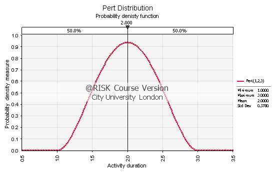
Fig. 3.1: PDF of the Pert Distribution with activity time estimates a=1, m=2 and b=3

3.5.2 Triangular Distribution

Another widely used distribution by Project Managers that uses three-point estimates in @Risk is the Triangular Distribution. The following graph (Fig. 3.2) illustrates the PDF with the same input data as Pert’s graph above.

The prevalent characteristics of the Triangular Distribution are that firstly, it produces a slightly higher probability measure around the most likely activity time estimate, compared to Pert. Secondly and most importantly, it has fatter-tails towards the extreme events, meaning that it takes into consideration the optimistic and pessimistic time estimates to a greater extent than Pert. Besides, it can be seen directly in the illustrated examples that the Triangular Distribution gives out a higher standard deviation value compared to Pert. Therefore, it can be deduced that the Triangular Distribution may produce more realistic outcomes than Pert does, as it models the behaviour of extreme events more precisely, as proposed by Schatteman et al. [12].

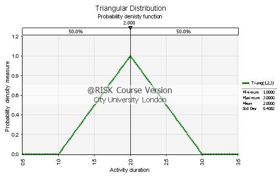
Fig. 3.2: PDF of the Triangular Distribution with activity time estimates a=1, m=2 and b=3

3.5.3 Uniform Distribution

The Uniform Distribution differs from the other three because it does not demand the same three-point estimates to be modelled. Conversely, @Risk requires a lower and an upper limit, so that the interval of the Uniform Distribution would be defined. Hence, the optimistic and pessimistic activity time estimates could be used to represent these limits. An example of the Uniform Distribution PDF can be seen below in Fig. 3.3.

The most important characteristic of the Uniform Distribution is that all the events within the specified interval have the same occurrence probability. In other words, the Uniform Distribution could be used to model events that happen equally likely within the given duration interval. Hence, the reason for which the Uniform was selected, was that it could potentially produce a more pessimistic model compared to the other three distributions.

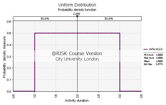
Fig. 3.3: PDF of the Uniform Distribution with time interval a=1 and b=3

3.5.4 Lognormal Distribution

Finally, the Lognormal Distribution was selected, as the final probabilistic input to be analysed. More specifically, numerous researchers, such as Triesch and Baker [17] and Mohan et al. [1], have indicated that the Lognormal is an appropriate distribution for probabilistic scheduling of construction projects.

Similarly, with the Uniform, the Lognormal Distribution requires only two parameters to be modelled. In this case, the mean (μ) and the standard deviation (σ) are needed to produce the PDF in @Risk. For comparative reasons, it was decided to feed the two parameters of mean and variance, as generated by the PERT method, into the interface of @Risk. Therefore, the resulting Lognormal PDF, shown in Fig. 3.4 below, would follow PERT’s estimates closely and would be easy to model.

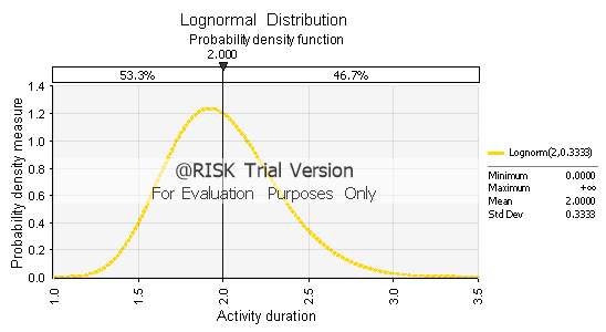
Fig. 3.4: PDF of the Lognormal Distribution with μ=2 and σ=0.3333

3.5.5 Distribution Comparison

After having declared the four types of probabilistic distributions to be used in the analysis that follows, it was decided to set out a direct comparison amongst them, to draw meaningful conclusions.

In Fig. 3.5 in page 25, the four symmetrical distributions are illustrated together using an activity duration interval between 1 and 3 days. It is apparent that the Lognormal has the lowest standard deviation value, whereas the Uniform has the highest amongst the four. Therefore, it can be implied that the former would produce more optimistic results, the latter more pessimistic and Pert and Triangular would fall in between the two.

In Fig. 3.6 in page 26, a similar fitting of the four distributions is depicted, though the pessimistic time estimate is set to be equal to 5 days. Therefore, the Pert, Triangular and Lognormal distributions follow an asymmetrical shape and their behaviour becomes apparent. Pert has a mean value of 2.333, whereas the Triangular has a slightly higher at 2.667, while the latter generates a considerably higher standard deviation value 0.8498 compared to 0.7127. The Uniform Distribution produces the largest mean and standard deviation, with values that reach 3 and 1.1547 days respectively.

The values given above and seen in the two figures that follow could be justified by the shape of the generated probabilistic curves. The Pert Distribution has a steep increase in the optimistic time estimate, has a peak around the most likely one and follows a significant fall towards the pessimistic area. On the contrary, the Triangular distribution follows a smoother incline, has a lower peak on the most likely area, and finally has a fatter tail towards its end. Therefore, it can be induced that the Triangular would produce more stochastically pessimistic results than Pert.

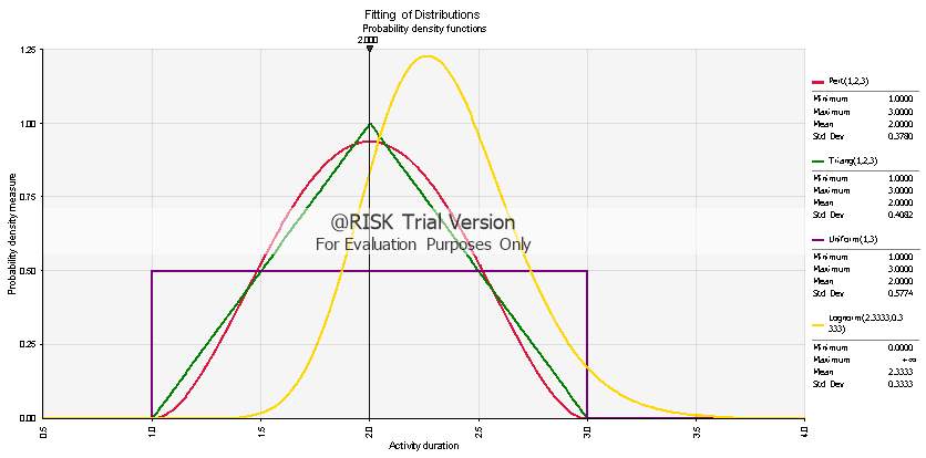
Fig. 3.5: Symmetrical activity distribution fitting for Pert, Triangular, Uniform and Lognormal distributions within a 1 to 3 time-unit interval

 

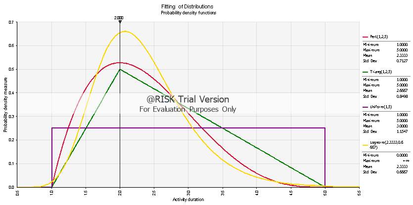
Fig. 3.6: Asymmetrical activity distribution fitting for Pert, Triangular, Uniform and Lognormal distributions within a 1 to 5 time-unit interval

3.6 Fast and Accurate Risk Evaluation (FARE) Technique [4]

Aside from the PERT method and the Monte Carlo Simulation, over the years, numerous novel scheduling tools have emerged in the scientific community of project risk analysis. As identified in Section 2.3, a fairly interesting probabilistic scheduling methodology is the one described by Jun and El-Rayes [4], called Fast and Accurate Risk Evaluation (FARE) technique.

The FARE Technique is a simplification of the usual network analysis in which large project networks are reduced by removing paths that could be represented by others. Essentially, this is achieved by two criteria. The first criterion is the Upper Probability Bound (UP), in which paths that have very high completion probabilities, greater than the UP value, could be represented by other paths on the network. The second criterion corresponds to the inherent correlation Upper Correlation Bound, (UC) amongst project paths. More specifically, in complex projects where the paths are contingent to each other due to sharing of common activities, highly correlated paths could be neglected. Again, the paths that generate a correlation value higher than the user-defined UC threshold should be removed from the project network. Therefore, the FARE technique is able to reduce the complexity of the project networks by using these two criteria.

As far as the creation of the FARE technique is concerned, the authors based themselves on three different scheduling components; the standard PERT method (described in Section 3.2), the multivariate normal integral method, which is the basis of the MCS, and the use of an approximation method on large-scale networks. The latter deals with the identification of the representative paths, or in other words, with those paths that are used to represent the ones that need to be removed. This approximation method is computer-based and some of its key points are illustrated in Appendix A. However, a brief description of FARE technique’s algorithm is outlined below.

The technique consists of three main phases of several steps. In “phase 1”, the user of the technique specifies the values for the two criteria, UP and UC. Also, redundant links that create parallel paths with a higher probability of completion should be deleted from the project network. Next, the user moves onto “phase 2” which deals with the removal of high-probability paths. This phase constitutes of three steps, as follows.

In the first step, the user changes the UP into an equivalent lower bound for mean path duration (LM). In the second step, the longest path duration search (LPDS) algorithm is employed, to determine the longest mean path duration (LD_n) and the largest variance (LV) for every resulting combination of paths. Note that these two values correspond to the entire project network and are fed into the following step.

The third and final step analyses the representative paths by relying on the fast representative path search (FRPS) algorithm. The latter guides the user through the analysis process to determine which paths should be analysed or removed directly. The LM value is used as a threshold and is compared against the expected mean duration of the path at hand. If the former is higher than the latter, the path is removed from the project network, and the node at which the path starts off should not be analysed again. Otherwise, the path is kept as a representative path. The flowcharts of the two algorithms are given in Appendix A.

As a final third phase of the method, the user proceeds with the removal of highly correlated paths. Correlations amongst paths should be computed at first, to determine which paths could be represented and thus be removed from the network. The authors relied on the original method devised by Ang et al. [20] with a small, but considerable alteration. They suggested that the user should sort the resulting correlation table in ascending order of the path probability of completion. Therefore, the user could select the most appropriate representative paths.

Hence, users of FARE can produce simplified project networks and avoid potentially lengthy simulations, without compromising in accuracy compared to the MCS results. For this reason, in this dissertation it was decided to implement an approximation of the FARE Technique (FARETA), due to non-availability of the appropriate software, in order to test the reliability of the proposed method.

3.6.1 FARE Technique Approximation

Based on the methodology illustrated by Jun and El-Rayes [4], the author proceeded to the application of a simplified approximation technique, to achieve the desired network path reduction. The methodology at hand was applied to both construction projects. Further, the results of FARETA are compared against those generated by a full MCS using the Pert Distribution.

The main limitations that led to the simplification were firstly due to the non-availability of an appropriate scheduling interface, to simulate the original technique and secondly due to the complexity of the two newly-developed algorithms. MS Project does not enable its users to isolate individual network paths. Consequently, it was not feasible to proceed with the application of the LPDS and FRPS algorithms, and their application has to be done manually. Hence, the approximation was deemed essential so that the analysis could be applied effectively to both construction project networks. This approximation is illustrated below in the following eight steps.

• Step 1: Setting of the upper probability bound (UP) value.
• Step 2: Setting of the upper correlation bound (UC) value and calculation of the path correlation using the formulas below.

ρk,l=Covk,lσkσl

(5)

Covk,l=∑i=1nak,nal,nσn2

(6)

where,

ρk,lis the correlation between paths

kand

l;

Covk,lis the covariance between paths

kand

l; and

ak,n=1if activity

nis on path

k, otherwise

ak,n=0.

• Step 3: Application of PERT analysis (as illustrated in Section 3.2) on every single path to determine the mean, standard deviation and probability completion time (substitute of the LPDS algorithm).
• Step 4: Formation of a table (as shown in Table 3.1 below) that includes the mean, standard deviation, probability of completion and correlation amongst paths, as shown below, and sort it in ascending order with regards to the probability measure.

Table 3.1: Correlation analysis results

	Mean (μ)	St. Dev.(σ)	Probability (%)	ρ1,n	ρi,n	ρk,n
Path 1
Path i
Path n

• Step 5: Indicate the representative paths of the project network by comparing the probability of completion with the UP value and the resulting correlation value with the specified UC. Remove any paths whose P(t≤T) is greater than UP (substitute of the FRPS algorithm).
• Step 6: Remove any paths in which ρ is higher than UC as they can be represented by other paths with the same value of ρ and a lower UP measure.
• Step 7: Update the MS Project network and run an MCS using @Risk, to calculate the overall completion probability, using the Pert Distribution.
• Step 8: Compare the results with those produced by the full MCS using the original project network and specify the margin of error.

At this point, it is suggested that the eight steps shown above would approximate the original FARE Technique close enough. Hence, any distortions to the resulting outcomes could be avoided successfully.

As a last step of the FARETA analysis, it was decided to perform a sensitivity analysis between 10,000 and 100,000 iterations, to determine whether there is a significant change in the simulation duration, or not. That way, the initially proposed objective by Jun and El-Rayes [4] regarding the reduction of simulation duration could be validated as such.

In Chapter 4, the results of the conducted quantitative risk analysis on the two construction projects are extended in great detail.

Input distributions may be correlated with one another, individually or in a time series. Correlations are quickly defined in matrices that pop up over Excel, and a Correlated Time Series can be added in a single click. A Correlated Time Series is created from a multi-period range that contains a set of similar distributions in each time period.