Statistical Process Control and Engineering Process Control
Info: 5499 words (22 pages) Example Dissertation Proposal
Published: 24th Jan 2022
Tagged: EngineeringStatistics
CHAPTER ONE - INTRODUCTION
1.1 Research Background
Chemical industry has employ multiple method of process control. Process control is important to maintain a specific result and to ensure the obtained product is within the set point. This will determine the value of the product and can either increase or decrease it. This make the process control as an important aspect to be considered during any chemical process and can influence the success or the failure of the process. Generally, two of the main process control widely used in industries are the Statistical Process Control (SPC) and the Engineering Process Control (EPC). SPC is standard methodology for measuring and controlling quality during the manufacturing process. It is a fairly simple process thus will not need a high cost to install.
Basically, SPC will measure the result obtained with the set point and present it as data, usually in the form of graph. By the graph, operator can determine whether the process is following the set point. In case of any deviation from the desired set point, the operator need to adjust it manually the manipulated variable and correct the deviation back to the desired set point. In general, SPC act as a visual aid to help the operator in maintaining the process control. On the other hand, Engineering Process Control (EPC) is a collection of techniques to manipulate the adjustable variables of the process to keep the output quality such as Feedback control process. EPC can collect data from the instrument, compare it to the set point and send signal for correction action. This mean that, EPC can automatically control the process to maintain it at the desired set point.
1.2 Objective
- To integrate both Statistical Process Control and Engineering Process Control for batch process control to detect possible variation as early as possible.
- To develop a methodology that integrate both Statistical Process Control and Engineering Process Control for batch process.
1.3 Problem Statement
For batch process, the variation or faults usually different from batch-to-batch that causes by several process variables. If the variation is not detected earlier, it is hard to maintain the quality of the end product between batches. This can cause the whole batch to fall below the requirement set point and would be a loss to the company. A better control process is needed that can predict the outcome of each batch process based on the disturbance and can automatically act accordingly to reduce the discrepancy.
1.4 Scope of Research
This research main focuses is on the implementation of both EPC and SPC for a batch process. The tuning methods used are Ziegler-Nichols (Z-N), Direct Synthesis (DS), and Internal Model Control (IMC). For the mathematical model used for the batch process will be obtained from past literature and re-constructed using SIMULINK MATLAB. For the statistical analyzation, MINITAB will be used to analyse the process capability and stability. At the end of this study, it is expected that integrating both process control can increase the efficiency and the capability of the batch process.
1.5 Significance of Study
Batch process is one of the process used in the industry to produces many type of chemical. Among the chemical that rely on batch process to be produces are pharmaceutical product, paints and adhesives. There is always desire to increase the efficiency and capability of the batch process. This will reduce the cost and loses for the affected industry. SPC and EPC has been research regularly as a method for process improvement and quality control. Recent publications have also reported that integration of SPC and EPC would produce an increase in performance compared when only used one process control only. This has increase interest and many have publish a study on integration of SPC and EPC. However, most of the study focus on continuous system. The integration of SPC and EPC for a batch process is not yet fully explored. This study hope to explore on this and come up with useful information and finding. Through the information and finding, it is hope to bring benefit to the chemical manufacturing industries and to provide needed exposure for future research in this field.
CHAPTER TWO - LITERATURE REVIEW
2.1 STATISTICAL PROCESS CONTROL
Statistical process control (SPC) was first developed by Dr. Walter A. Shewhart in 1920s as a tool to monitor the quality and the variability of process. SPC is useful as it display the process in a binary view of whether the process is in control or out of control. Using SPC, ones can figure out easily when the process is not conforming to the required process standard and corrective action can be taken. SPC do this by the help of statistical tools, control charts (Škulj et al., 2013). Control chart consist of three important part, the mean value or the centreline, the Upper Control Limit (UCL) and the Lower Control Limit (LCL) as shown in figure below:
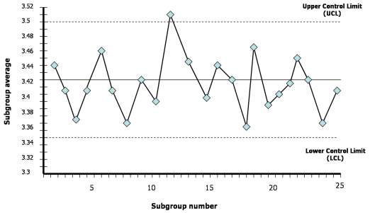
Figure 2.1 Basis of a control charts.
From figure 2.1, the UCL and LCL act as the boundary of the process line which as long as it does not go beyond the UCL and LCL, the process is considered successful. Whenever the process is detected to deviate above the UCL or below LCL, it signifies that the process is out of control and needed a correction action immediately. Subgroups can be defined as a collection of homogeneous data. Homogenous data means that the data is made up of things that are similar to each other.
For every sample, several reading is needed to ensure accurate data collection and this group of readings is considered as subgroup. For example, a subgroup sample size of 5 means that there are 5 reading for every point at a time. Different subgroups will determine the type of control charts suitable to be used. Throughout the year, many type of control charts are developed. Each with their own formulae for the mean, UCL and LCL. Different type of control chart have their own purpose or specialty and can sometimes use together with another control chart. This is important to provide both qualitative and quantitative analysis of the process (Azizi, 2015). Among the control chart commonly used are the X-bar (X̅) chart, Range (R) chart, Individual (I) chart, Moving Range (MR) chart, Cumulative Sum (CUSUM) chart, and Exponentially Weighted Moving Average (EWMA) chart.
2.1.1 X̅ Chart
X̅ chart is also known as the average chart. This is because it utilised the average or the mean value of each sample to produce the chart. It is commonly used for monitoring the quality of a product within a subgroup. X̅ chart is useful because it can be used to measure many type of qualitative parameters such as temperature, height, weight, flowrate and many more. However, in order for it to get enough information, it should be used when there are more than 10 samples available. Usually, this control chart is used together with the other types of control charts such as the R chart (Montgomery, 2009). To calculate the mean value, the following formula is used:
| X̅=∑i=1nXinX̅=X1+X2+X3……Xnn | (2.2.1) |
Where: X̅=mean valueXi=observation temperature, height, etc. i=1,2,…,nn=number of observation The centreline and control limit are obtained using the equation:
| Centreline, X̅̅=∑i=1kX̅ik | (2.2) |
| UCL for X̅ chart =X̅̅+A2R̅ | (2.3) |
| LCL for X̅ chart=X̅̅-A2R̅ | (2.4) |
Where: X̅̅=centreline of the chartR̅=average of range i=1,2,…,kk=number of subgroupA2=control chart constant from Table 2.1 Table 2.1 Constant values for X̅ and R charts.
| Subgroup Size | A2 | d2 | D3 | D4 |
| 2 | 1.880 | 1.128 | 0 | 3.268 |
| 3 | 1.023 | 1.693 | 0 | 2.574 |
| 4 | 0.729 | 2.059 | 0 | 2.282 |
| 5 | 0.577 | 2.326 | 0 | 2.114 |
| 6 | 0.483 | 2.534 | 0 | 2.004 |
| 7 | 0.419 | 2.704 | 0.076 | 1.924 |
| 8 | 0.373 | 2.847 | 0.136 | 1.864 |
| 9 | 0.337 | 2.97 | 0.184 | 1.816 |
| 10 | 0.308 | 3.078 | 0.223 | 1.777 |
Source: (Hossain et al., 1996) From the formula, the X̅ Chart can be plotted. Figure 2.2 below shows an example of X̅ Chart with one point outside of the upper limit:
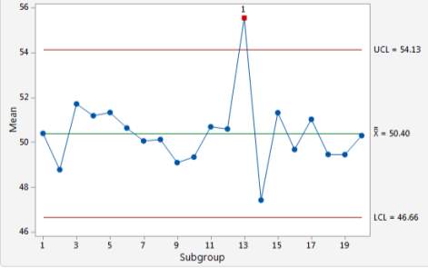
Figure 2.2 Example of an X-bar Chart
2.1.2 R Chart
R chart or also known as range chart is used to measure the variation of a sample within a subgroup. To get the variance, the highest value of the subgroup is subtracted with the lowest values. This is what it mean by range. The range is then inserted into the equation to calculate the centreline, UCL and LCL to plot the R chart.
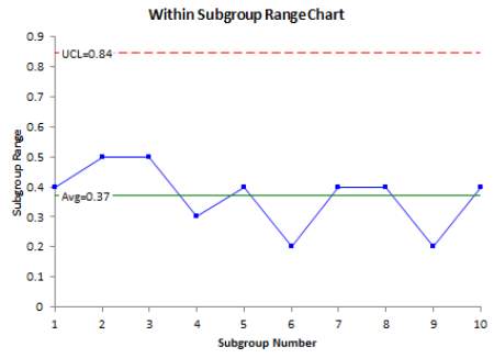
Figure 2.3 Example of R Chart To plot the R Chart, the following equation are used:
| R=Xmax-Xmin | (2.5) |
| Centreline, R̅=∑i=1kRik | (2.6) |
| UCL for R Chart=D4R̅ | (2.7) |
| LCL for R Chart=D3R̅ | (2.8) |
Where: R̅=average of range i=1,2,…,kk=number of subgroupD3 D4=control chart constant from Table 2.1
2.1.3 I Chart
The I chart or individual chart is basically the same as X̅ chart. However, I chart is used when it is impractical to collect a multiple sample (Montgomery, 2009). That mean I chart is more suitable to be used when there are a small subgroup size. Larger sample size is good for sensitive chart, but smaller subgroup size may be necessary for a very slow processes or it is very expensive to obtain measurement.
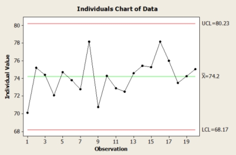
Figure 2.4 Example of I Chart The control limit for the I chart is calculated using the following equation:
| Moving Range, MR=|Xi-Xi-1| | (2.9) |
| MR̅=X1-X2+X2-X3……|Xn-Xn-1|n-1 | (2.10) |
| Centreline, X̅=∑i=1kX̅ik | (2.11) |
| UCL for I Chart=X̅+3MR̅d2 | (2.12) |
| LCL for I Chart=X̅-3MR̅d2 | (2.13) |
Where: MR̅=average of moving range i=1,2,…,kk=number of subgroupn=subgroup sized2=control chart constant from Table 2.1
2.1.4 MR Chart
MR chart, or also known as moving range chart is used to monitor variation within the sample by calculating the difference between two consecutive data. In practice, it is usually combined with I chart to become an I-MR chart where the I chart helps assess the process centre and the MR chart plots the process variation.
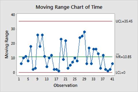
Figure 2.5 Example of a Moving Range Chart
| Centreline, MR̅=X1-X2+X2-X3……|Xn-Xn-1|n-1 | (2.14) |
| UCL for MR Chart=D4MR̅ | (2.15) |
| LCL for MR Chart=D3MR̅ | (2.16) |
Where: MR̅=average of moving rangen=subgroup sizeD3 D4=control chart constant from Table 2.1
2.1.5 EWMA Chart
The EWMA control chart is typically used for an individual observation. This mean that it is used when there is only individual sample of subgroups. EWMA have the performance approximately equivalent to CUSUM control chart although it is easier to set up and operate compared to CUSUM chart (Aljebory et al., 2014). To calculate the EWMA, it is important to decide on a weighting factor, λ. This is used to determine the weight given to previous data.
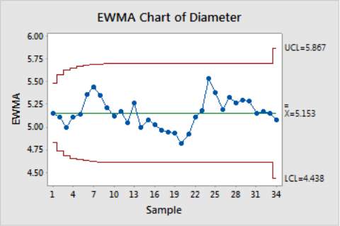
Figure 2.6 Example of EWMA Chart The equation needed for EWMA Chart are as follow:
| Zt=λXt+(1+λ)Zt-1 | (2.17) |
Where: Zt=EWMA at the time tZt-1=EWMA at the time (t-1)Xt=sample result at time tλ=the weighting factor (0
| Centreline=μo | (2.18) |
| UCLt for EWMA Chart=μo+3σλ(2-λ)[1-(1-λ)2t] | (2.19) |
| LCLt for EWMA Chart=μo-3σλ(2-λ)[1-(1-λ)2t] | (2.20) |
Where: μo=the control targetσ=the standard deviationλ=the weighting factor (0
2.1.6 Process Capability Analysis
Process capability analysis is used to determine the quality and efficiency of a process. Capability studies are usually used to assist during the stages of product design, such as to deciding the acceptable norms, selecting process and operators (Mahesh et al., 2010). Process capability analysis use the six- sigma (6σ) spread as a way to measure the process capability. It is done by comparing between the difference of Upper Specification Limit (USL) and the Lower Specification Limit (LSL). Not to be confused with control chart limits, because control chart limits is based on estimate of variation from the given process itself while specification limits are typically derived by user (engineer, manufacturer, etc) itself. The difference is used to compare with the 6σ and several possibility may occur. The possible scenarios and the respective meaning are tabulated below for clearer understanding: Table 2.2 Comparison of Process Capability with its explanation.
| Scenarios | Explanation |
| 6σ > (USL – LSL) | The process is not capable of achieving the specifications. |
| 6σ = (USL – LSL) | The process is said to be able to meet the exact specifications. |
| 6σ | The process is capable of meeting the specifications. |
A convenient way of expressing the capability of the process is by using process capability indices (PCI) denoted as Cp, and Cpk. Cp is known as the capability index. It is used to express how well the data fits between the USL and LSL. Cpk is the centering capability index. Cpk compares both the spread of the process and the location of the mean relative to the specifications (Pearn et al., 1998). The formula used to determine the Cp and Cpk are listed below:
| Cp=USL-LSL6σ | (2.21) |
| Cpk=min USL-X̅3σ,X̅-LSL3σ | (2.22) |
Where: X̅=meanσ=standard deviation From the value of Capability index Cp and Cpk calculated, the estimation of the process can be estimated as shown in the table 2.3: Table 2.3 Estimations of Process based on Cp and Cpk (Johnson et al., 2001)
| Capability index | Estimation of the Process |
| Cp | The process is not capable of achieving the specifications. |
| Cp ≥ 1.33 | The process is satisfactory enough |
| Cpk = Cp | The process is placed exactly at the centre of the specification limits |
| Cpk | The Process is not capable of achieving the specification |
| Cpk > 1.33 | The process is capable |
When using process capability index, several factors should be considered. This is because it usually depend on the sample size as it can affect the value of Cpk. Larger sample size is recommended for a better result. Furthermore, it is only applicable when the process is normally distributed. According to (Mahesh et al., 2010), using it on a process that is not normally distributed may often lead to inaccurate results. The process capability is expressed using the process capability chart. From the capability chart, the process can be observed whether I falls within or exceed the specification limits. Depending on several criteria, the process ability could be determined. The criteria are the process data is stable and in control, the data are normally distributed and the specification limits fall on either side of the centreline (Montgomery, 2009). Figure 2.7 show an example of process capability chart where the graph distribution is within the USL and LSL.
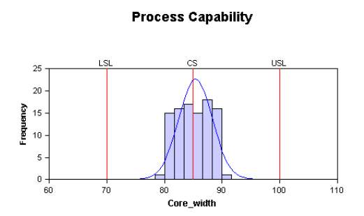
Figure 2.7 Example of Process Capability Chart.
2.2 ENGINEERING PROCESS CONTROL
Engineering Process Control (EPC) or also known as automatic process control is a popular technique used for process optimization and improvement. It describes the manufacturing process as an input-output system where the input variables can be manipulated to counteract disturbances (Aljebory et al., 2014). This is achieved through controller actions which carry out continuous adjustments to the manipulated variable. The output process is used as the final product measurements. There are various types of controller for EPC, such as PID, fuzzy logic, ANN, etc. Among them, PID controller are the most popular and usually used in industry. This is because PIC controller has a simples design, cost effective and provide satisfactory performance.
The notations P, I and D for a PID controller are representative of its variables which are the process gain (Kc), time integral (τI) and derivative time (τD). Each variable is responsible in governing the stability and response of the process. There are many methods the PID controller can be configured. For example, feedback system, feedforward system and internal model control system. Among them, feedback is the simplest control strategy and widely used. Each of these methods possess their own advantages and disadvantages.
2.2.1 Feedback Control System
Feedback system operate in a closed loop manner where a controller is actively making adjustments to the process variable. The term “feedback” was derived from the condition whereby the controlled variable is measured and fed back to the controller and thus will adjust the output accordingly. According to (Smith et al., 1987), the output value is compared against the input whereby any error between the two will be compensated by adjusting the manipulated variable. The advantages of feedback control is it has a simple design thus it is easy to tune, especially for fast and short dead time processes. Due to this, feedback controller is commonly used in oil refining, chemical processing and many more. However, feedback controller also have its disadvantages, such as it can only take any corrective action once the process deviate from the set point. This is sometimes unwanted because it effect the product quantity as material defect and long recovery time. Another disadvantages of EPC is it does not remove the root cause but just simply adjusting to it continuously.
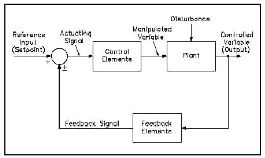
Figure 2.8 Block Diagram of Feedback Control System
2.2.2 Internal Model Control System
Internal Model Control (IMC) system are example of PID controller that been gaining popularity recently. IMC method is to achieve a fast and accurate set point tracking by removing the effect of disturbance as effectively as possible (Korsane et al., 2014). An advantage of IMC method is that it allows uncertainty and trade-offs between performance and robustness to be considered in a systematic approach (Smith et al., 1987).
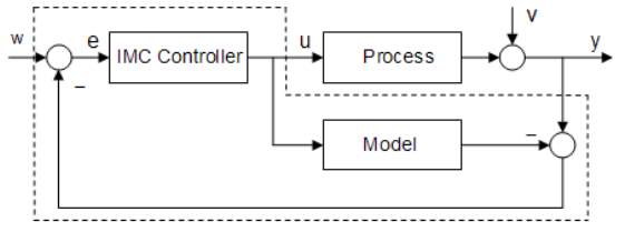
Figure 2.9 Block Diagram of Internal Model Controller.
2.3 BATCH PROCESS
Batch process in chemical industries is a process that depend the amount of time that produced products by bulk and not in continuous (Vinson, 2008). The batch process involves charging the feed into the reactors or vessel, processing them under controlled conditions, before discharging them as final product. The process is considered a success if only the values of the process variables remain within the acceptable limits and resulting with a high-quality product while following the recipe prescribed for the respective processes (Mears et al., 2017).
Example of chemical process that utilised batch process are the production of polymers, pharmaceutical and food manufactures, semi-conductor industries, biochemical reactors and many more. Batch processes may seem simple at first, however, managing the product quality monitoring and production scheduling and organization make it quite a complicated process (Wu et al., 2017). Moreover, batch process is usually not entirely automated and require intervention by the process operator in order to ensure the quality of the end product and to avoid of an out of spec product. Hachicha (2012) stated that most batch processes run in an open-loop fashion, because of the lack of on-line information and need to be obtained off-line from laboratory assays of few product samples.
In the process control field, there is a need for innovative monitoring and control techniques of the batch process operations. This is because batch and semi-batch processes play a significant role in the production of high value added materials and product (Hachicha, 2012). Furthermore, consumer pressure has resulted in a greater emphasis on product quality (Lennox et al., 2000). According to Wang et al. (2017), a primary challenge for batch process monitoring techniques is to define which is the “normal” operation from which operating cycles that are evaluated and can be identified as successful or failed. A quality control strategy for a batch process often reduces to the on-line control of the trajectories of the key process variables. This is because it may be difficult to detect quality shifts and to counteract it if there are no on-line or real time information.
With the real time information, it is possible to perform the intervention midcourse of the batch process to compensate for the change detected. In recent years, there are high focus on this area, namely Multivariate statistical process control (MSPC). MSPC is different to traditional SPC where it identifies all of the critical variables and underlying patterns in a data set while SPC relies on data such as mean, median, standard deviation, etc., (Duran-Villalobos et al., 2016). MSPC show all process variables, including relationships which cannot be detected with traditional SPC.
This removes the need for control charts for every individual variable because traditional SPC approaches involve plotting trends of important quality parameters and ensuring that these trends do not violate the pre-set control limits. Example of MSPC technique widely applied are, multi-way principal component analysis, multi-way partial least squares, and model predictive controllers (Hachicha, 2012).
2.4 INTEGRATED SPC/EPC
SPC and EPC originate from different industries and have been developed independently in the past. Nowadays, SPC and EPC are widely practiced in manufacturing industry to control a process. Both while act as a control process, have a very different approach, where SPC monitors the process and identify the assignable causes while EPC optimizes the process by manipulation the process variable to compensate the effect of disturbance (Montgomery, 2009). According to (Hachicha, 2012), SPC should not be used to adjust dynamic process and EPC cannot be used to detect assignable causes.
Although both methods are satisfactory process control, it is evidence that both can be considered as two complementary strategies for process control. This is because SPC is able to monitor the process but cannot adjust it automatically while EPC could continuously and automatically adjust the process but cannot determine the root cause or removing it (Montgomery, 2009). It makes sense that by integrating both EPC and SPC would result with a better control system where the SPC would monitor the process and determine the assignable causes, and EPC will automatically corrected it. According to (Hachicha, 2012), integration of EPC/SPC can be done by three method, algorithmic SPC, Active SPC and Run-to-Run. Based on this three method, Run-to-Run is seemed as the most suitable to be used in batch process.
2.4.1 RUN-TO-RUN
Run-to-Run, or also known as Run-By-Run process control techniques have been developed and applied mostly to semiconductor manufacturing processes. Semiconductor product is usually a wafer and each run could consist of a batch of wafer undergoing the same process conditions. Run-to-Run control system operate such as that a control action or change in process parameter can only be implemented between runs instead of during a run (Hachicha, 2012). In this process control, SPC act as a monitoring tools using the suitable control charts detecting the need for Run-to-Run control action. Meanwhile, EPC will perform the adjustment needed to the inputs or initial conditions between run.
CHAPTER THREE - METHODOLOGY
3.1 Overview
This study was carried out in two phases, namely the off-line monitoring phase and the on-line measuring and detecting phase. The offline detecting phase is consist mainly of collecting data. A collection for the past successful batch process is done in this part and the process key monitoring variables will be selected. From the data collected, the control limits for each selected key variables (SPC) and the control adjustments of the process (EPC) is determined using Minitab. The on-line measuring and detecting phase is where the model of the integrated SPC and EPC is run using SIMULINK MATLAB R2015a. Here, fault detection and diagnosis of the SPC/EPC integration will be done. After that, the process will be evaluated again using Minitab whether the key variables is within the SPC limits. The process will be modify based on the SPC/EPC integration if the process is not within the SPC limits. Figure 3.1 will show the process flow of the SPC and EPC integration proposed.
3.2 Process Flow
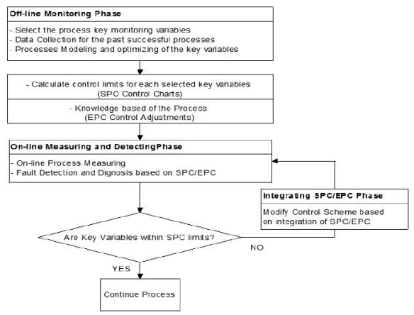
Figure 3.1 Flowchart for the proposed SPC/EPC integration approach Source: (Aljebory et al., 2014).
REFERENCES
Aljebory, K. M., & Alshebeb, M. (2014). Quality Improvement ( A Case Study : Chemical Industry - National Chlorine Industries ). Jordan Journal of Mechanical and Industrial Engineering, 8(4), 243–256. Azizi, A. (2015).
Evaluation Improvement of Production Productivity Performance using Statistical Process Control, Overall Equipment Efficiency, and Autonomous Maintenance. Procedia Manufacturing, 2(February), 186–190.
Duran-Villalobos, C. A., Lennox, B., & Lauri, D. (2016). Multivariate batch to batch optimisation of fermentation processes incorporating validity constraints. Journal of Process Control, 46, 34–42.
Hachicha, W. (2012). Batch processes monitoring based on statistical and engineering process control integration: case of alkyd polymerisation reactor. International Journal of Automation and Control, 6(3/4), 291.
Hossain, a., Choudhury, Z. a., & Suyut, S. (1996). Statistical process control of an industrial process in real time. IEEE Transactions on Industry Applications, 32(2), 243–249.
Johnson, D. W., Jeffries, A., Minsek, D. W., & Hurditch, R. J. (2001). Improving the process capability of SU-8, part II. Journal of Photopolymer Science and Technology, 14(5), 689–694.
Korsane, D. T., Yadav, V., & Raut, K. H. (2014). PID Tuning Rules for First Order plus Time Delay System. International Journal Of Innovative Research In Electrical, Electronics, Instrumentation And Control Engineering, 2(1), 582–586.
Lennox, B., Hiden, H. G., Montague, G. A., Kornfeld, G., & Goulding, P. R. (2000). Application of multivariate statistical process control to batch operations. Computers & Chemical Engineering, 24(2–7), 291–296.
Mahesh, B. P., & Prabhuswamy, M. S. (2010). PROCESS VARIABILITY REDUCTION THROUGH STATISTICAL PROCESS CONTROL FOR QUALITY 1 . 4 Process Capability Indices. International Journal for Quality Research, 4(3), 193–203.
Mears, L., Stocks, S. M., Sin, G., & Gernaey, K. V. (2017). A review of control strategies for manipulating the feed rate in fed-batch fermentation processes. Journal of Biotechnology, 245, 34–46.
Montgomery, D. (2009). Introduction to statistical quality control. John Wiley & Sons Inc. Pearn, W. L., & Chen, K. S. (1998).
New generalization of process capability index Cpk. Journal of Applied Statistics, 25(6), 801–810.
Škulj, G., Vrabič, R., Butala, P., & Sluga, A. (2013). Statistical process control as a service: An industrial case study. Procedia CIRP, 7, 401–406.
Smith, C. A., & Corripio, A. B. (1987). Principles and practice of automatic process control. Automatica, 23(3), 414.
Vinson, J. (2008). The Value of Batch Process Design in a Chemical Engineering Education, 1–8.
Wang, R., Edgar, T. F., Baldea, M., Nixon, M., Wojsznis, W., & Dunia, R. (2017). A geometric method for batch data visualization, process monitoring and fault detection. Journal of Process Control.
Wu, S., Jin, Q., Zhang, R., Zhang, J., & Gao, F. (2017). Improved design of constrained model predictive tracking control for batch processes against unknown uncertainties. ISA Transactions, 69, 273–280.
Cite This Work
To export a reference to this article please select a referencing stye below:
Related Services
View all


Related Content
All TagsContent relating to: "Statistics"
Statistics is a branch of applied mathematics concerned with the collection and analysis of numerical data. The term statistics is also used to describe the facts that are obtained from the collection and analysis of that data.
Related Articles

DMCA / Removal Request
If you are the original writer of this dissertation proposal and no longer wish to have your work published on the UKDiss.com website then please: