Monte-Carlo Methods for Option Pricing

Abstract

This thesis presents a review of above mentioned Monte Carlo based algorithms for pricing American options and provides implementations with simple examples of American put options.

The purpose of the study is to test the effectiveness of these techniques and the dependencies on various simulation parameters. 

Many problems in mathematical finance entail the computation of a particular integral. In many cases these integrals can be valued analytically, and in still more cases they can be valued using numerical integration, or computed using a partial differential equation (PDE). The famous Black-Scholes model, for instance, provides explicit closed form solutions for the values of certain (European style) call and put options. However when the number of dimensions in the problem is large, PDEs and numerical integrals become intractable, the formulas exhibiting them are complicated and difficult to evaluate accurately by conventional methods. In these cases, Monte Carlo methods often give better results, because they have proved to be valuable and flexible computational tools to calculate the value of options with multiple sources of uncertainty or with complicated features.

A number of Monte Carlo simulation-based approaches have been proposed within the past decade to address the problem of pricing American-style derivatives. The purpose of this paper is to discuss some of the recent applications of Monte Carlo methods to American option pricing problems. Our results suggest that the Least Squares Monte Carlo method is more suitable for problems in higher dimensions than other comparable Monte Carlo methods.

In finance, derivatives are contracts between two parties whose value is dependent upon a single or a group of underlying assets. They can be used, in the right circumstances, to hedge risk, generate profit and provide leverage for the holder. Derivatives played a key role in the 2007-2009 financial crisis, inherently pricing these derivatives accurately is imperative. Pricing derivatives is an interesting area of research in financial mathematics. In recent years, much research has been done in order to be able to accurately and efficiently price increasingly complicated contracts.

In this project, we look at one of the more popular classes of derivatives, Options. The project outlines a number of different methods which have been developed to price standard and more complicated options. Particular focus is put on the Monte-Carlo method and its efficiency in its approximation. Using examples, we investigate how to option price is dependent on certain variables in the underlying asset. We discuss the drawbacks these methods possess, study the error in the methods and consider variance reduction techniques in order to improve the methods.

 

 

 

 

 

 

 

 

 

 

Contents

 

1 Introduction                                                                           p
1.1 Options                                                         p
1.2 The Black–Scholes Model                                  p
1.3 Monte-Carlo Methods                                                  p
1.4 Monte-Carlo Methods                                                  p
1.4 Monte-Carlo Methods                                                  p

2 Pricing European Options                                             p
2.1 ………………………………………………    p
2.2  ………………………………………………                                p
2.3  ………………………………………………                                p
2.4  ………………………………………………       p

 

3  Monte Carlo methods                                                 p
3.1 ………………………………………………      p
3.2 ………………………………………………      p
3.3 ………………………………………………      p

 

4 A Numerical Example and Results of LSM                              p        4.1               ………………………………………………                                             p
4.2  ………………………………………………      p
4.3  ………………………………………………      p
4.4  ………………………………………………      p
4.5  ………………………………………………      p

 

 Conclusion                                                            p

 Acknowledgements                                                       p

 References                                                               p

 Appendix  Matlab codes   

 

 

 

Chapter 1

 

Introduction

 

1.1 Background

Financial Options

An option is a contract which gives the holder the right but not the obligation to buy or sell one share of an asset at an agreed price, called the exercise price (denoted by E) at an agreed time, called expiry (denoted by T). There are two types the option can take: A call option, or a put option. A call option gives the holder the right to buy the stock at the agreed, whereas a put option gives the holder the right to sell.

There are different styles an option can take and therefore different ways of pricing them. The most common are European and American options. European options allow the holder to exercise only at expiration. In contrast to this American options allows the holder to exercise at any timebefore expiration. Both European and American options are commonly referred to as Vanilla options. There also exist variations of the above styles In terms of what dates they can be exercised, what price they can be exercised at and how payoff function is calculated? These are referred to as Exotics options. Examples of these include Bermudan, Asian, Barrier, Binary, Digital and many more. The aim of this project is to outline the different types of options, investigate how the Monte-Carlo can be used to price a number of these and to look at how American options can be priced using the Longstaff-Schwarz method.

Asset pricing model

Before proposing a suitable asset pricing model, it is important to first understand what a stochastic process is. Stochastic processes can be classified into discrete time or continuous time processes.

A discrete time stochastic process is a sequence of random variables

X0,X1,…,XNwhich are observations of some random system at certain points in time

t=0,1,…,N.

A continuous time stochastic process is a set of random variables

Xtt>0, which are observations of some random system at any time

t>0.t∈R

A Markov process is a type of stochastic process which the future evolution of the process after time m, depends only on the observation at time m and is independent of any observation before this time. That is (in discrete time):

PXm+1=xm+1,…,Xn=xnX0=x0,…,Xm=xm=PXm+1=xm+1,…,Xn=xnXm=xm

In the construction of the asset price model, we assume that stock prices follow a stochastic process, more specifically a Markov process.

Assuming the efficient market hypothesis, that prices adjust instantaneously to new information about the market, we can model the asset price as a Markov process in the sense that future evolutions of the stock price are independent previous stock prices.

Attempting to model the asset price as a random walk, yield two potential problems. Firstly, the is nothing to stop the random walk taking negative values, something which would not happen in the real world since when the stock price reaches 0, it will remain 0 indefinitely. Secondly, the size of the change will be proportional to the price since larger prices would mean a larger change than at a small price. Therefore, it is reasonable to assume that it is the return of the asset that acts as a random walk rather than the price itself.

Letting

δtbe a small increment of time,

Si=Siδtbe the asset price at time

iδt,

μbe the expected value of the return on the asset per unit of time and

σbe the variance of the asset price per unit of time. Then over

δtthe expected return on the asset price is therefore

μδt. We set

T=Nδt, hence

SThappens at the

Nth time step. The variance of the return at this step should be N times that over a single time-step, so we expect the variance for one time-step to be proportional to

δt. The random component in the return over one time-step should then be proportional to

δt.

Using these facts we arrive at our model for the discrete time price of an asset.

Sn+1-SnSn=μδt+σ δt Yn+1

Where

Yiare i.i.d. random variables which take values ±1 with probability ½.

1.2 Methods of pricing options

Black-Scholes Method

Two notions which are important to understanding the derivation of the Black-Scholes formula are that of Brownian motion and Itô’s lemma.

A Brownian motion is a continuous time stochastic process which the following are true:

1. there is a constant σ > 0 such that, for any real numbers

   s,

   t ≥ 0, the random variable

   Wt+s-Wthas normal distribution

   N0,σ2t;

2. given any sequence of times

   0≤t0≤…≤tn, the random variables

   Wtr-Wtr-1, for  1 ≤ r ≤ n, are independent;

3. W0=0;
4. Wtis a continuous function of t with probability 1 (i.e. in almost all possible paths).

To simulate Brownian motion in MATLAB, we use an approximation in discrete time. If we fix a small time step

δt, then our approximation for

Wnδtis:

S0=0;     Sn=Sn-1+σδtξn      for  n ≥1

where the

ξiare i.i.d. random variables from a standard normal distribution

N0,1.

Itô’s lemma is an identity used in Itô calculus to find the differential of a time-dependent function of a stochastic process.

Itô’s Lemma: Let

Xt=ft,Wtbe a stochastic process, then

dXt=∂f∂t+12∂2f∂Wt2dt+∂f∂WtdWt

Recall our equation for the discrete-time asset pricing model. For the derivation of the Black-Scholes model, we must consider the continuous-time version of this model. To do this we just replace

δtYn+1by increments of a standard Brownian motion

Wtt>0and let

δt→0, resulting in the following equation:

dSt=Stμdt+StσdWt

.

Using Itô’s lemma it can be shown that the solution to

dSt=Stμdt+StσdWtis:

St=S0eμ-σ22t+σWt

.

To derive the famous Black-Scholes equation we consider an option with a payoff at expiry equal to

VT,ST, with underlying asset St following equation 1.4.

Consider a portfolio P consisting of Buying one unit of the option and short selling a units of asset St. This value of this portfolio at t being:

Πt=Vt,St-aSt

Over a small time period

δt,

dΠt=dVt-adSt

Using Itô’s lemma it can be shown that:

dVt=∂V∂t+μSt∂V∂St+12σ2St2∂2V∂St2dt+σSt∂V∂StdWt

Combining these two equations we get:

dΠt=∂V∂t+μSt∂V∂St+12σ2St2∂2V∂St2-aμStdt+σSt∂V∂St-aσStdWt

For the portfolio to be hedged we want to eliminate the random component. Therefore, the coefficient of

dWt= 0

⇒a=∂V∂St

and the amount of underlying asset which must always be held is

: -∂V∂St.

⇒dΠt=∂V∂t+12σ2St2∂2V∂St2dt

.

Again, we know that there is no risk in the portfolio and there are no arbitrage opportunities, therefore, the return made by the portfolio must be equal to the risk-free rate.

⇒dΠt =rΠtdt

This is equivalent to:

∂V∂t+12σ2St2∂2V∂St2dt=Vt-St∂V∂Stdt

Drop the subscript t and we arrive at the famous Black Scholes equation:

∂V∂t+12σ2S2∂2V∂S2+rs∂V∂S-rV=0

The model is based on a number of assumptions that don’t hold up in the real world but this partial differential equation governs the evolution of the exact price of a European call or put option. Together with suitable boundary conditions this equation can be transformed into the heat equations by applying several transformations.

The formula is then in a form ready to be solved, the solution then is:

Vt,S=SNd1-Ee-rT-tNd2

With

d1=logSE+r+12σ2T-tσT-t

and

d2=d1-σT-t

Limitation of the Black-Scholes Model

It is crucial to keep in mind that this model assumes that the risk-free rate and

volatility are assumed to be constant over the option`s life-span. This assumption is very

unlikely to be encountered in option trading. Furthermore, the other major assumption is

that the option can only be exercised at the maturity, but not all options have the same

maturity date. In fact, this model loses its magic when dealing with vanilla options:

American options, since they can be exercised anytime during their lifetime. It is possible

to evaluate European option using the Black-Scholes-Merton model because European

options can be exercised only at the end of their lives. In contrast, the Black-Sholes

Merton model fails in the process of valuation American options because American

options have a more flexible exercise rule and can be exercised at any time before the

expiration date.

 

One-Step binomial method

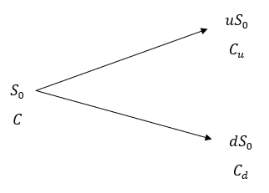A favoured method for the valuation of options is the Binomial method. It is based on the assumption that the stock price is modelled by a random walk throughout the lifetime of the option. At each time step

δtthe stock price would have even risen by a certain amount, we can denote this as

uS0or fallen to a certain amount, denoted by

dS0(illustrated in the figure below).

By setting C equal to the option price and using the assumption that no arbitrage opportunities exist we can construct a portfolio such that we know the value of the portfolio at time T. Since there is no risk in this portfolio the return is equal to the risk-free rate.

Consider a portfolio consisting of buying

xshares and short selling 1 option. The idea is to find

xsuch that the value of the portfolio is the same if the stock price increase or decreases. This is called hedging.

We set

Cuand

Cdequal to the payoff from the option if the stock price increases or decreases respectively.

If the stock price increases the value of the option is
S0ux-Cu

If the stock price decreases the value of the option is

S0dx-Cd

Setting these two equations equal to each other and we arrive at

x=Cu-CdS0u-S0d

We know that there is no risk in the portfolio and there are no arbitrage opportunities, therefore, the return made by the portfolio must be equal to the risk-free rate.

Let

rbe equal to the risk-free rate, then the present value of the portfolio is

S0ux-Cue-rT

The cost of setting up the portfolio is

S0x-C

Setting these two equations equal yields

C=S0x1-ue-rt+Cue-rt

Substituting in equation (1.7) we obtain the following result

C=p*Cu+1-p*Cdert

Where

p*=ert-du-d

p*

is called the risk-neutral probability and equations (1.8) and (1.9) form the basis of how to price options using the Binomial method for a single time step and a higher number of timesteps.

The binomial method approximation converges to the Black-Scholes value as the number of time steps, N, tends to infinity, see the general theory in Kwok (1998), Clewlow and Strickland (1998), Lyuu (2002) and Higham (2004). However, it is widely reported that the convergence is not monotone and the sawtooth pattern in the sequence of approximations makes the binomial approximation less attractive.

Monte-Carlo Methods

There is no hard and fast definition of Monte-Carlo Simulation, but in general, it is usually the process of repeating randomly generated samples and then performing some statistical analysis on these samples.

This method has been used in a number of industries such as finance, engineering, supply chain, and science. In finance, its main use is to find the expected value of a function

fx, from a distribution density

ξxover

x∈R.

Eξfx=∫fxξxdx = u

Generally, the above integral is approximated by:

1. Sampling an element

   xifrom the distribution density

   ξx

2. Simulate function

   fxiby putting in your element from

   ξx

3. Repeat steps 1 and 2 M times (where N is desired number of iterations)
4. Calculate mean of the values of this function

   fx

   (1.10)

Efx̂=1N∑i=1Nfxi=û

A key theorem upholding the validity of the Monte-Carlo method is Kolmogorovs’ Strong Law of Large Numbers.

Definition: Let

X1,X2,…be a sequence of random variables, and

Xis a random variable then we say

Xn→Xalmost surely as

n →∞if

P{ω∈Ω :XNω→Xω}=PXn→X=1

We say that say that

Xnconverges to

Xin probability if for any

ϵ>0we have

limn→∞⁡P{ω∈Ω :Xnω-Xω≤ϵ}=1

Kolmogorovs’ Strong Law of Large Numbers: Let

{Xi}i=1∞be a sequence of independent identically distributed (I.I.D) random variables with expectation

EXi=μand Var

Xi< ∞. Then for all

ϵ>0we have, as

n →∞

1n∑i=1nXi→X       (a.s.)

Error in the Monte-Carlo method

The error estimate in the Monte-Carlo method is given by the standard deviation of the average of all the simulations.  This is given by:

s2=1n-1∑i=1nfxi-û2

The central limit theorem ensures that the distribution of

û-usnfollows the standard normal distribution for large n.

Hence,

Pû-z1-α2sn<u<û+z1-α2sn≈1-α

To investigate the accuracy of how well u approximates

ûwe first need to take the expectation of

û-u:

Eû-u=Eû-u

=E1N∑i=1Nfxi-u

=1N∑i=1NEfxi-u

Since

ûIID  it has its own mean and variance,

Efxi=u. There the method is unbiased.

Next, we look at the variance of

û-u:

Varû-u=Varû-Varu

=Var(û)                 since

Varu = 0

=Var1N∑i=1Nfxi

=1N2 Var∑i=1Nfxi

Since

fxiare independent:

=1N2Ns2=s2N

where

sis the standard error in the estimate. Therefore, error scales as

ON.

1.3 Variance Reduction Techniques

The smaller the variance between the number of simulations the smaller the standard error is and therefore the more accurate the answer. A number of techniques have been developed in order to reduce the variance of the method and therefore the number of simulations it takes to achieve the same level of accuracy. In this project, I look at two of these methods in detail.

Antithetic Variable Technique

A standard property of the Gaussian distribution is that given an evaluation of a Gaussian variate

zigiven by

vi=vzi,then we also have

vî=v-zi. If we view

viand

vînot as individual samples, but taking

vî=12vzi+v-zias an individual sample then with one evaluation of

vîrequires 1 gaussian drawn generation but two calculations.

This technique results in a reduction in variance if

V12vi+vî<12Vvi

Or equivalently

Covvi,vî<0

This is the case when

vzis monotonic.

The resulting Monte-Carlo method is as follows;

û=1N∑i=1Nfxi+f-xi2

Control Variate Technique

In the case where a solution can be found analytically, we are able to use the Control Variate technique.

Say you want to find

EX=1N∑i=1Nfxi

given that we already know

EY≔ y

where

Xand

Yare in some way correlated.

We say Y is the control variate.

Therefore, we can define some new random variable Z as

Z=X+βY-EY

Applying the expectation to both sides yields

EZ=EX+βEY-EY=EX

Now, applying the Monte-Carlo method to Z yields the following

VarZ=VarX+βY=VarX+2βCovX,Y+β2VarY

Choosing the value of

βwhich minimizes the variance gives

βmin=-CovX,YVarY

Hence

VarZ=VarX-Cov2X,YVarY

Therefore, there is a reduction of variance if

CovX,Y≠0.

Typically, we do not know the covariance between variables X and Y, this can be however estimated in the Monte-Carlo Method itself.

 

 

 

 

 

 

 

Chapter 2

 

Monte-Carlo methods for option pricing

 

The most common use of Monte-Carlo methods in finance is undoubtedly in the pricing of options. Typically, the outline of this method is as follows:

1. Sample random path for

   Stin a risk-neutral world.

2. Calculate payoff function

   Vt,ST

3. Repeat steps 1 and 2 M times
4. Calculate mean to get the expected value of the payoff
5. Discount the expected payoff at the risk-free rate to get the risk-neutral price of the option.

The price evolution paths over time period T are calculated in the same way as before, setting by:

dSt=Stμdt+StσdWt

.

⇒St=S0e μ-σ22t+σWt

In a risk-neutral, the drift parameter

μnow becomes

r. With the approximation of

Wtthe equation becomes:

St=S0er-σ22t+σ normrnd0,1T

The main benefits of this approach are that the method’s ability to value options with a non-standard payoff. In particular, this method can be adapted to price options where early exercise is available, such as in American options. The downside to this approach is that process of simulating for large M is computationally demanding. In an industry such as finance when every millisecond counts for generating profits, it’s imperative to make these algorithms work as efficiently as possible.

2.1 Monte-Carlo Method for European Call

The European option is perhaps the simplest of all types of options to understand. The payoff function of a European call is simply given by:

Payoff=maxST-K,0

This ease of valuing this option comes from the fact that the option is restricted to being exercised at the end of the contract, T.

A number of models have been proposed to accurately price the European option, the most notable being the Black-Scholes methodology. This model, as previously discussed has the ability to give the exact value of the option price with exceptional speed.

The following section will investigate how the Monte-Carlo method is used to price European options and how this price is affected by a change in the number of iterations and share prices variables. It will also compare the Monte-Carlo method and the 1 step binomial method with the exact value of the option using the Black-Scholes formula.

To begin my investigation, I designed Monte_Carlo_European_Call.m which along with all other codes, can be found in the appendix. To ensure the code was giving me the correct output from the Black-Scholes formula I used the same inputs that are used in (Higham, 2004). Keeping all variables fixed and Increasing the number of iterations in the Monte-Carlo method yielded the following graphs. Together they show how the option price converges to the exact value given by the Black-Scholes formula as the number of iterations increase. I chose the value of

M=10,000as the number of iterations since this ran for a total 56.528 seconds and gives us a sufficiently accurate approximation, increasing

Mto 100,000 would have been better if I was working on a higher performance computer.

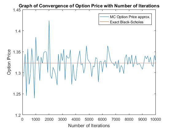
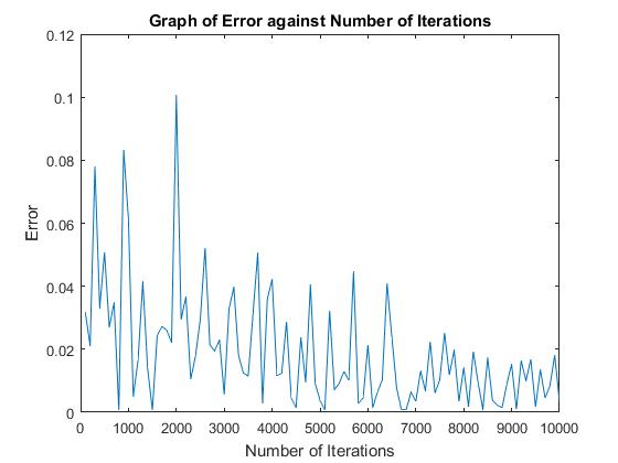
Figure 1       Figure 2

Figure 1 shows how as we increase the number of iterations from 100 to 10,000 the approximation of the option price, given by the Monte-Carlo method approaches the true option price, given by the Black-Scholes method. The deviation of the approximation from the constant value of 1.3231 gets smaller and smaller. Figure 2 shows a similar result as the number of iterations increases the absolute error of the approximation tends to 0.

If  Figure 2 is adapted so that it instead of plotting the error against the number of iteration we now plot the log of both of these quantities we obtain Figure 3.

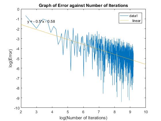
Figure 3

Using MATLAB’s data fitting tool, it is shown that the error scales as what we would expect from the Monte-Carlo method. Earlier it was proved that the error of the Monte-Carlo method scales of

O1M, as we have a gradient of -0.53 fitted to figure 3 the simulations agree with proof.

The following set of graphs outline the option price changes when all parameters are kept the same bar one.

From figure 4 we can see increasing the share price leads to a higher value for the option, intuitively this makes sense since the higher the stock price, the more likely you will be to exercise the option at expiry.  Increasing the stock price had little effect on the relative error in the model. Figure 5 shows a similar relation to figure 4. Increasing the exercise price leads to a fall in the option price since we are less likely to exercise the option at expiry. Like figure 4 this had little effect on the relative error apart from the trivial case when we are close to boundary

Option Price =0.

Figure 6 shows how the option price changes when the interest rate is increased. Increasing the interest rate

rincreases the option price this is because as interest rates rise, the opportunity cost of buying the stocks increases since investors are lose out money they would get from the T-bills interest. Therefore, call options become more valuable. Again, there is no notable effect on the relative error of the Monte-Carlo Method.

Increasing volatility also increases option price, as shown in figure 7. This is because when volatility is high the likelihood of extreme value is increased, the share price is bounded at 0 and therefore that is the lowest extreme, but there is no cap to the share price when there are high extreme values and therefore the likelihood of a higher payoff is increased, consequently the price of the option will increase. The relative error increases dramatically when volatility is large.

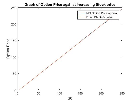
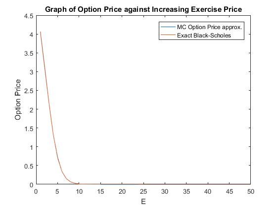
Figure 4      Figure 5

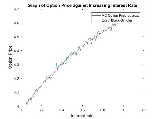
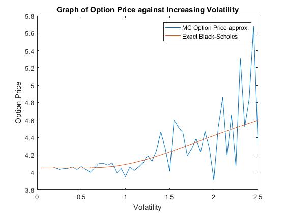
Figure 6                     Figure 7

 

 

 

 

 

 

 

 

 

 

 

 

Variance Reduction: Monte-Carlo Method for European Call

S0=5,  E=4,  r=0.05,  σ=0.3,  T=1,  Black-Scholes Solution= 1.3231

Table 1

M		Crude Arithmetic Monte-Carlo	Antithetic Monte-Carlo
10,000	Option Price	1.3247	1.3263
	Standard Error	1.3707	0.5206
	Confidence Interval	1.2979 – 1.3516	1.3161 – 1.3366
	Time (s)	0.042	0.054
100,000	Option Price	1.3206	1.3220
	Standard Error	1.3833	0.5136
	Confidence Interval	1.3120 – 1.3292	1.3188 – 1.3252
	Time (s)	0.188	0.183

From Table 1 we can see that even with 100,000 simulations the crude Monte-Carlo method confidence intervals are too large and do not give us the required accuracy of 2 decimal places. The Antithetic Monte-Carlo method greatly reduces the standard error in the method and therefore the variance. The level of accuracy given by the Antithetic Monte-Carlo from 10,000 simulations is close to the level given by that of the crude Monte-Carlo method with 100,000 simulations at a fraction of computational time. The time required to complete 100,000 simulations for both methods is the same, whereas the Antithetic version achieves this with a lower standard error and is accurate to the required 2 decimal places. Since the European Call option can be modelled by the Monte-Carlo method, it has no practical use since a quicker, exact method exists.

 

 

 

 

 

 

 

 

 

Comparison with the Binomial Method

Running Binomial.m with the same input as the ones used in the above Black-Scholes and Monte-Carlo method shows how the binomial method converges to the exact Black-Scholes solution and the number of time times increases (shown in figure 8). The output shown in figure 9 shows that the error scales as 1/N which agrees with the value given in the literature. (CHANG, 2007)

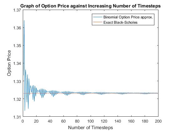
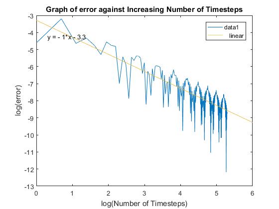
Figure 8      Figure 9

When comparing the Black-Scholes, the Binomial and the Monte-Carlo methods there is a big discrepancy between the efficiency of the three models. The most efficient as expected is the Black-Scholes formula since this is simply the closed form solution and direct computation. This process was exact and took 0.002 seconds to generate the answer. The binomial was next, taking 0.009 seconds to reach an approximation which is exact to 3 d.p. using a total of 124 time steps. The binomial model does not have a closed form solution (Georgiadis, 2011). To reach the same level of accuracy as the binomial method the Monte-Carlo method must have a number of 10,000 simulations, taking a total of 22.301 seconds to run. Even at this number, the solution isn’t always accurate to 3 d.p.

This is a perfect example of where the Monte-Carlo method can be useless in the real world, the method is hugely computationally demanding and should only be used when necessary.

2.2 Monte- Carlo Method for Asian Options

An Asian option is a type of an Exotic option whose payoff depends on the average price of the underlying asset over the lifetime of the contract. This payoff function generally takes the form:

Payoff=maxA0,T-E,0

Where

A0,Tis the average price over the lifetime of the contract.

This average can be one of two types, arithmetic or geometric average. The arithmetic average is given by:

A0,T=1N∑t=1NSt

The geometric average is given by:

A0,T=∏t=1NSt1N

This averaging helps to lower the volatility of the option and as a result the option price tends to be cheaper than that of the European or American options.

The valuation of the Asian option proves to be more difficult than in the case of European. For the arithmetic average there does not exist a closed form analytic solution, therefore numerical methods must be applied to approximate a solution. A closed for solution does exist however for the geometric average.

A number of researchers have proposed methods to approximate the solution to the problem. The standard binomial method is not suitable in the valuation of arithmetic Asian options since the number of paths which must be averaged grows exponentially with the number of time steps. It would simply take too long to reach a good approximation. (John C Hull, 1993), (Levy, 1992), (Willmott, 1998) and others outline various methods to price Asian options. This paper investigates on the how the Monte-Carlo method is used to generate an approximation.

Closed Form Solution of the Geometric Average Asian Option

The payoff geometric average is given by: (…) , where

{ti}i=1nare such that

ti=iΔtand

nΔt =T.

Writing

∏i=1nSti=StnStn-1Stn-1Stn-22Stn-2Stn-33 .  .  .  St3St2n-2St2St1n-1St1St0nS0n

And using the fact that

If

X1∼Nμ1,σ12and

X2∼Nμ2,σ22then

X1 +X2∼Nμ1+μ2,σ12+σ22.

It can be shown that

log∏i=1nSti1n1S0=Nr-σ22n+12nT,σ2n+12n+16n2T

Furthermore, under a risk-neutral setting the price of Asian call option is the same as the price of the European call when volatility of European option’s underlying stock

σ̂satisfies:

σ̂2=σ2n+12n+16n2

And drift

μ̂given by

μ̂=12σ̂2r-σ22n+12n

The closed form geometric Asian option price is given by the following:

VT,S0=e-rTS0eμ̂TNd1̂-ENd2̂

Where

d1̂=logS0E+μ̂+12σ̂2Tσ̂T

d2̂= d1̂ – σ̂T

This project looks at how the Monte-Carlo method can be used to price both arithmetic and geometric average Asian option. I investigate how the option varies when the underlying assets variables is increased. Additionally, how the error of the geometric Asian option converges to 0 as the number of Monte-Carlo simulations and number of time-steps increase.

I start off by looking at the geometric Asian option. I use the same inputs as before and set the number of time-steps to 10. To ensure the code was running correctly, I set the volatility of the underlying asset to zero, which makes the share price deterministic, this gives a standard error of 0 and the approximation is equal to the exact value. Here the number of time-steps refer to the number of time period that are being averaged over.

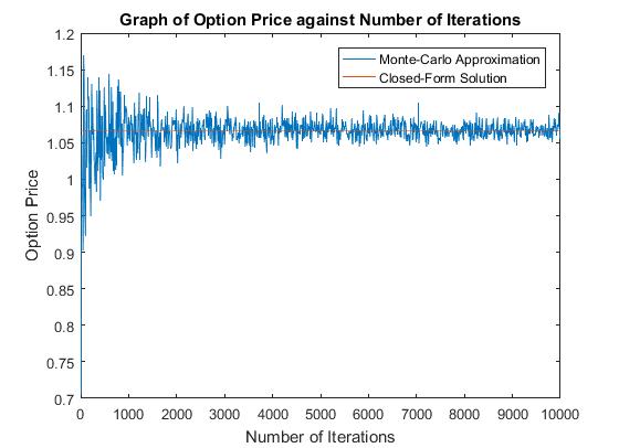
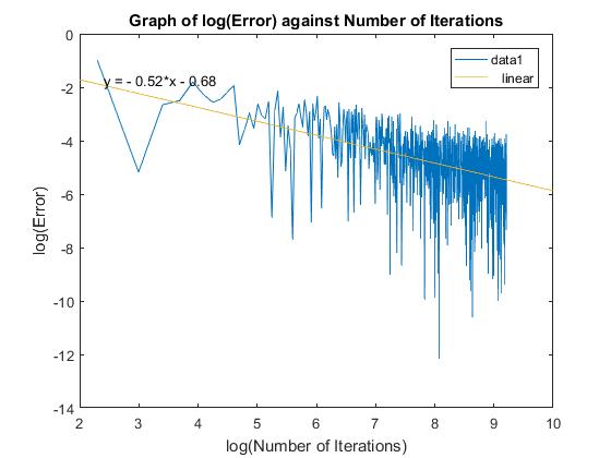
Figure 10 and 11, show a similar result to that of the standard European Call option. The first thing to note is that option prices is comparably lower than that of the European, due to the reduction of extreme positive payoff values. We can see that as the number of simulations increase the option price approaches the true value given by the closed form solution. Again, the error scales as

O1M.

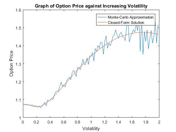
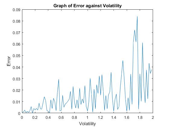
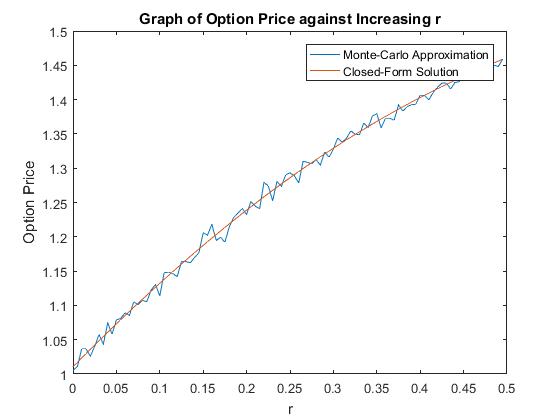
Increasing the volatility of the asset price increases the option price and the error, as it did for the European case.

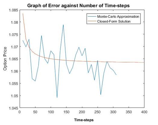
An interesting point to note is how the closed form solution decreases as the number of Time-steps increases. Intuitively this makes sense since the averaging nature of the Asian will help to mitigate the affect they might have on the payoff and applying a similar argument we with the Monte-Carlo and the strong law of large numbers, the more time-steps used the less of an effect these jumps will have. The error is independent of the number of time steps.

Using 100,000 simulations and 100 time-steps, it takes 7.042 s to obtain an accurate to 3 decimal places. This gives us a standard error of 0.8070 and a 95% confidence interval of [1.0600,1.0700]. This is not accurate to the appropriate number of decimal places and 1,000,000 takes far too long to run, therefore further work needs to be done to the model in order to reduce the variance.

The Arithmetic Asian option

Proof of why average us bigger

Variance Reduction: Monte-Carlo Method for Arithmetic Asian Option

S0=5,  E=4,  r=0.05,  σ=0.3,  T=1,  Analytical Geometric Solution= 1.0632

Table 2

M		Crude Arithmetic Monte-Carlo	Crude Geometric Monte-Carlo	Antithetic Monte-Carlo	European Call as Control Variate	Geometric as Control Variate
10,000	Option Price	1.1129	1.0547	1.0996	1.0952	1.0957
	Standard Error	0.828	0.7979	0.1967	0.4336	0.055
	Confidence Interval	1.0966 – 1.1291	1.0391 – 1.0703	1.0958 – 1.1035	1.0867 – 1.1037	1.0947 – 1.0968
	Time (s)	0.952	1.613	1.629	1.252	1.612
100,000	Option Price	1.0971	1.059	1.0953	1.0952	1.0956
	Standard Error	0.8251	0.8024	0.1914	0.433	0.054
	Confidence Interval	1.092 – 1.1022	1.054 – 1.064	1.0941 – 1.0965	1.0926 – 1.0979	1.095 – 1.0959
	Time (s)	9.044	11.87	14.475	8.865	15.826

We can see from Table 2 that all three methods discussed offer a reduction in variance. The largest being from the method which uses the geometric average as the control variate. The covariance between the Geometric and Arithmetic average options is relatively large. This can also be seen in figure (…) where the option price for the arithmetic average always remains slightly above that of the geometric average. The reason for this is proved below.

The same level of accuracy as that of the crude Monte-Carlo with 100,000 simulations can be achieved by the Antithetic and the Geometric as a control variate method with only 10,000 simulations.  Looking at the 95% confidence intervals, one can deduce that the Arithmetic average option price for the aforementioned inputs is 1.10 accurate to 2 decimal places and 1.095 to 3 decimal places. This agrees with what we had in figure(…). The fastest method is the European Call as control variate method, but this offers the least reduction in variance, whereas a better level of accuracy can be achieved in a shorter time by the Geometric Average as a control variate in only 10,000 simulations taking 1.612 seconds as opposed to 8.65 seconds.

2.3 Monte-Carlo Method for Barrier Options

Barrier options are a class of exotic path-dependent options. Path dependence simply means that the option’s payoff is dependent on not only the underlying assets price at expiry T but also how it got there.

A Barrier option is very similar to the European option but with one key difference; If the underlying asset reaches a certain price throughout the lifetime of the option contract then the option either expires or it becomes active.

Generally, they are cheaper than the corresponding European option due to the fact that the asset price needs to satisfy the extra condition before becoming of value.

There are four main forms a barrier option can take:

1. Up-and-out: option expires worthless if the underlying asset price moves up and reaches a certain barrier.
2. Down-and-out: option expires worthless if the underlying asset price moves down and drops down past a certain barrier.
3. Up-and-in: option is only valid if the underlying asset price moves up and reaches a certain barrier, otherwise the option expires worthless.
4. Down-and-in: option is only valid if the underlying asset price moves down past a certain barrier, otherwise the option expires worthless.

Their nature means that Barrier options are more sensitive to changes in volatility. Increasing the volatility mean that extreme values are more likely. Therefore, for ‘’in’’ options, a positive payoff is more probable and so increasing volatility increases option price. For ‘’out’’ options, conversely, a positive payoff is less likely, so an increase in volatility leads to a decrease in option value.

Given a formula or value for an ‘’in’’ option then we can immediately find the corresponding ‘’out’’ option since when one option is knocked out/in, the other is knocked in/out. The two options follow the relation:

”in”+”out”=European

The stock needs to be monitored to check if it passes the barrier. The monitoring can happen discretely or continuously. Closed form solutions exist for the continuous monitoring case, however, due to financial and legal reasons, this is not implemented in reality. Instead, discrete monitoring is used. This however, is substantially more difficult since there is no practical closed form solution to this problem. (Ralf Korn, 2001)

The discreetly monitored case converges to the continuously monitored case when the time periods between monitoring decreases. The analytical solution is given by:

S0Nd1-Ne1-BS01+2rσ2 Nf2-Ng2-EerTNd2-Ne2-BS0-1+2rσ2Nf1-Ng1

Where

d1=log⁡S0E+r+σ22Tσ  T

d2=log⁡S0E+r-σ22Tσ  T

e1=log⁡S0B+r+σ22Tσ  T

e2=log⁡S0B+r-σ22Tσ  T

f1=log⁡S0B-r-σ22Tσ  T

f2=log⁡S0B-r+σ22Tσ  T

g1=log⁡S0EB2-r-σ22Tσ  T

g2=log⁡S0EB2-r+σ22Tσ  T

(Higham, 2004)

A number of methods have been developed to price Barrier options. This project focuses on the Monte-Carlo method, it compares the solution from the Monte-Carlo method to the analytical solution given above. We will also compare the solution to that of the adapted binomial and finite difference solution.

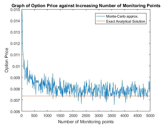
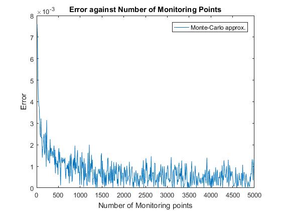
I first plotted the analytical solution given by the continuous monitoring case. Plotting the result from the Monte-Carlo method with an increasing number of monitoring points gave figures (!) and (!) show how the discretely monitored case converge to the continuous value as the number of monitoring points increases.

Next, I looked at how the option priced changed as we increased the barrier from 0 to

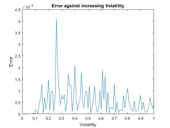
S0. Figure(!) shows how increasing the barrier on a down and out put option will decreases the price this is due to the fact that an increase in the barrier means that the barrier will be more likely to be crossed, hence the option is more likely to terminate worthless. The error in the Monte-Carlo method does not seem to be dependent on the barrier price. The error remains of a similar magnitude.

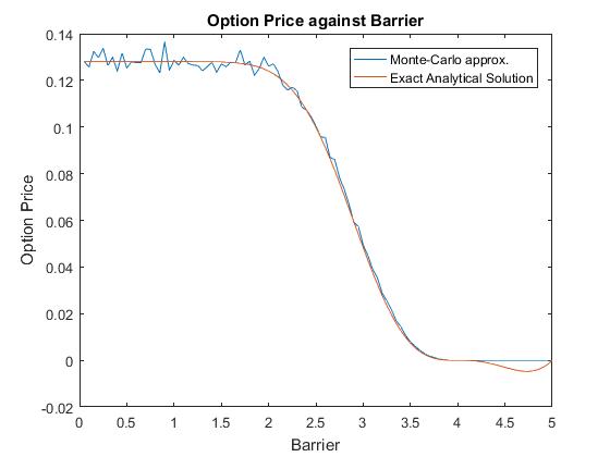
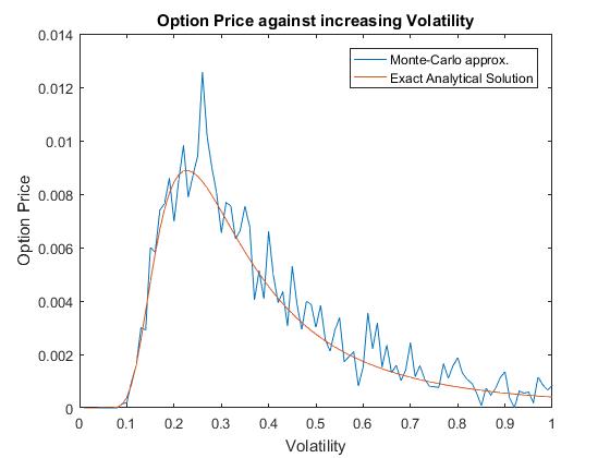
Similar to what was discussed earlier we see that the option price of the down and output option is quite sensitive to volatility movements. Figure(!) displays how different the values for the option price are with different values of volatility. For a down and output option when volatility is low, the option is less likely to be exercise since selling stock on the open market would be more profitable. However, when asset prices volatility is high, it is more likely that there are extreme values in the stock price, hence it is more likely that the barrier will be crossed, resulting in the option being worthless.

The Monte-Carlo method for pricing barrier options is a relatively efficient method with accurate results. It takes only 1.391 seconds with 10,000 simulations and 1,000 monitoring points to reach the desired accuracy of 3 decimal places against the continuously monitored case. Increasing the number of monitoring points beyond this is of little consequence.

Variance Reduction: Monte-Carlo Method for Barrier Options

S0=5,  E=4,  r=0.05,  σ=0.3,  T=1,  B= 3.5,  Closed form solution= 0.5214

Table 3

M		Crude Arithmetic Monte-Carlo	Antithetic Monte-Carlo	European Call as Control Variate
10,000	Option Price	0.5293	0.5289	0.5379
	Standard Error	0.6754	0.4521	0.6463
	Confidence Interval	0.5160 – 0.5425	0.5201 – 0.5378	0.5252 – 0.5505
	Time (s)	1.274	2.165	1.599
100,000	Option Price	0.5324	0.5319	0.5325
	Standard Error	0.6811	0.4510	0.6406
	Confidence Interval	0.5281 – 0.5366	0.5291 – 0.5347	0.5285 – 0.5365
	Time (s)	67.013	152.055	63.754

The Control Variate method offers only a small reduction in the variance, this implies that the covariance between the European call option and the Barrier Call option is relatively small. The Antithetic method does offer a reduction in variance, however, the cost of this is the increase in computational time which is quite significant. The total computational time doubles with only a mild reduction in variance. Using 100,000 simulations is more accurate than the corresponding Option Price for 10,000 simulations but more than 50 times faster. None of the 95% confidence intervals are small enough for the required accuracy of 2 decimal places. Therefore, although a barrier option can be modelled by the Monte-Carlo method, it has no practical use due to its inefficiency.

 

 

 

 

 

Chapter 3

 

American Options

 

Most of the options traded on the world’s exchanges are American options (Hull., 2012). These options are similar to the European option, the difference being that American options can be exercised at any time prior to the expiration date and European options are only exercisable at the expiration date (Benninga, 2014).

The payoff function for the American Call is given by:

Payoff=maxSt-E,0

The payoff function for the American Put is given by:

Payoff=maxE-St,0

Although the American option can take these two forms, it can be shown that it is never optimal to exercise an American Call early. The justification for this is as follows:

Suppose the holder of an American Call option wants to exercise at t<T. Giving

Payoff=maxSt-E,0

at time t.

Investing this risk-free until expiry yields:

Profit = maxerT-t*St-E,0

at time T

The alternatively, we could short-sell the asset at time t and invest the proceeds risk-free, buying the asset at time T.

Profit=St*erT-t+maxST-E,0-ST

at time T

Now, if

ST>E  then ,

Profit=St*erT-t-E

>erT-t*St-E

If

ST<E  then,

Profit = St*erT-t-ST

>erT-t*St-E

Hence, it is never optimal to exercise an American Call option early.

The flexibility American put options allow in their exercise time mean that there is a greater opportunity to make a profit in excess of that offered by its European equivalent. Therefore, the American option is generally more expensive than the European.

Despite being similar, the fundamental difference in their exercisability leads to extremely varied methods in pricing the options due to the additional problem of determining the optimal time to exercise the option. The holder must compare the payoff of the option from immediate exercising to the payoff if they were to continue to hold to a later date. Traditional methods previously mentioned such as finite difference and the binomial method start to break down when more realistic, multifactor (multi-dimension) problems are introduced because constructing approximate solutions to their underlying non-linear differential equations gets extremely difficult (Tilley, 1993).

3.1 Monte-Carlo for American Options

We are attempting to price American options, which can be exercised at any point t along a continuous time period [0,t]. This, however, is not practically possible, we must approximate this solution using discrete times at which the option can be exercised. This is somewhat is now essentially a Bermudan option. This difference inevitably leads to an error in our approximation which I will discuss later.

Tilley was the first researcher to publish a solution to the problem of using Monte-Carlo simulation to price American Options. His general approach was to compute estimates for the options price by using backward induction (similar to the binomial method) through the simulated evolution of a stock price over discrete time and a bundling process. He assumes that all randomly sampled stock price paths are equally likely with probability weight,

R-1. The option price was estimated by the following equation:

Option Price=R-1∑All paths t∑All paths kzk,tDk,tIk,t

Where

Dk,tis the path specific discount factor and

Ik,tis the payoff from the option.

To estimate the price of the option using (1), Tilley estimates the exercise-or-hold indicator function z(k, t) (which takes values of 0 or 1). Although this method was accurate for low dimensional problems, it struggled to be readily applied to higher dimensions and its major drawback was that it was very computationally demanding.

The research by Carriere (1996) and Tsitsiklis and Roy (1999) expands on the work of Tilley (1993) in determining the optimal stopping time. Carriere noted that the estimation of the exercise-or-hold indicator function,

zk,tshould be equivalent to the estimation of a series of conditional expectations. This advancement lead to a contribution to research in the area of pricing American options.

 

 

 

Longstaff and Schwartz Algorithm

In 2001 Longstaff & Schwartz published their paper, this method can readily be applied to options which depend on multiple factors, something which previous methods such as the binomial and finite difference methods have struggled to do.

Their approach assumes that the conditional expectation function mentioned above can be approximated using a least squares regression.

This conditional expectation function is given by:

CSti=EVi+1S(ti+1)S(ti)=s

,

Where

Viis the option value at time

ti.

Assuming that the continuation value can be approximated by a set of linear basis functions gives us:

ĈSti=∑n=1Nβnϕn

This assumption holds when the continuation value is an element of

L2space. Since

L2space is also a Hilbert space, it therefore has a countable orthonormal basis. Hence, the continuation value can be represented as a linear combination of elements in this basis.

We can choose a set of basis functions and apply regression to find coefficients

βnand hence, the continuation values.

Following (Longstaff & Schwartz, 2001) the set of basis functions we will use are the set of Laguerre polynomials given by:

LnS=exp-S2esn!dndSnSne-S

Therefore, we have

ĈSti=∑n=1NβnLnSti

In this project, I use the first 6 Laguerre polynomials given by:

n	LnS
0	1
1	(-S+1 )
2	12(S2-4S+2 )
3	16(-S3+9S2-18S+6 )
4	124(S4-16S3+72S2-96S+24 )
5	1120(-S5+25S4-200S3+600S2-600S+120 )
6	1720(S6-36S5+450S4-2400S3+5400S2-4320S+720 )

Other basis functions available include Hermite, Legendre, Chebyshev, Gegenbauer, and Jacobi polynomials.

After applying the regression and we have found

Cis, it is possible to compute whether or not it is best to immediately exercise the option or to hold.

Now we use the standard Monte-Carlo method to calculate the discounted option price using the optimal continuation value for each path. We only use the paths which give us a positive payoff, this is called pruning and it greatly increases computational speed.

The full algorithm is outlined below;

1. The first step of this algorithm, like the others, is to simulate a number of independent price evolution paths.

Calculate payoff at T the expiry date for each path. Only consider paths which the payoff is greater than 0.

2. Perform regression to obtain an estimation of coefficients

   βn

3. Calculate the estimation of continuation value

   Ĉ.

4. Calculate the immediate exercise value and hence the optimal stopping value.
5. If the immediate exercise value is greater than the continuation value, then payoff becomes the immediate exercise value. If it is not then the payoff becomes the payoff of the node 1 time-step ahead discounted by the appropriate amount.
6. Perform steps 2-5 recursively Working backwards from T to 0. At each time-step, for each path where payoff >0.
7. We now have a vector of length M, with optimal payoffs all appropriately discounted. Take the average of this and we obtain the option price for an American Put.

This entire algorithm is quite computationally demanding since the amount of computation increases exponentially as the number of price evolution paths and the number of time steps increases. Therefore, this model is not appropriate for the pricing simple American put options which are able to be solved by finite difference and binomial methods. However, as I mentioned before, the Longstaff-Schwartz method is able to approximate solutions to problems with increasing complexity why is why this method is so powerful.

To achieve the following results, I use 50 points at which the option can be exercised,

S=36, E=40, T=1, σ=0.2, r=0.06

The ensure the code is running correctly, the same values are used to that in (Longstaff & Schwartz, 2001). As an analytical solution does not for American options we will also use the Finite difference approximation (4.478) given in this paper to compare my approximation using the Longstaff and Schwartz algorithm.

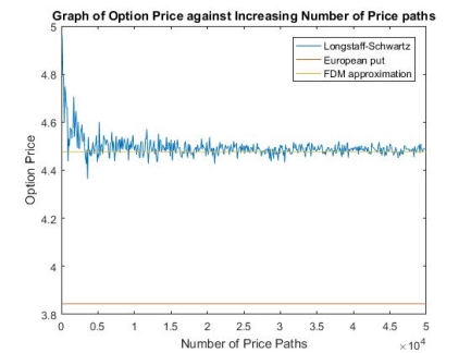
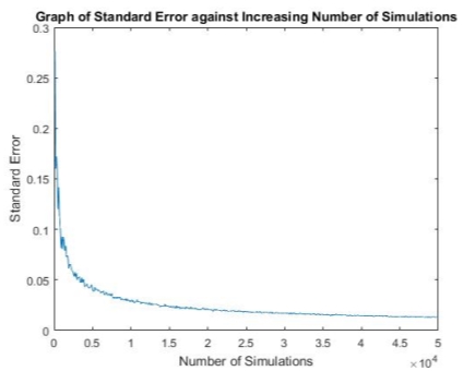
I first observed how the option price and standard error are dependent on the number of simulated price paths, M. Increasing M from 10 to 50,000 and keeping all other inputs the same yielded the figure(…) and figure (…).

A few key points to note is that Figure (…)  shows how the Longstaff-Schwartz method converges to the finite difference (FDM) approximation and M increases. It also confirms what was previously stated about how the equivalent European put is cheaper than the American option.

Figure (…)  shows how the standard error approaches 0 as the number of simulations is increased.

Next, I varied a number of different parameters to see how this would, in turn, affect the option price.

Figures (…),(…), (…) and  (…) all show similar results to that shown by the European case. These results are due to the same reasons discussed previously in the European case.

An interesting result is that shown in Figure (…), as the interest rates increase the prices of the American and European options diverge. An Explanation of this is that when interest rates are high, so is the from investing risk-free. Therefore, it is more beneficial to exercise the option early and invest risk-free. This extra benefit the American option has is reflected in the option price. Both prices decrease though due to the aforementioned opportunity cost.

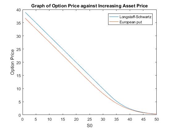
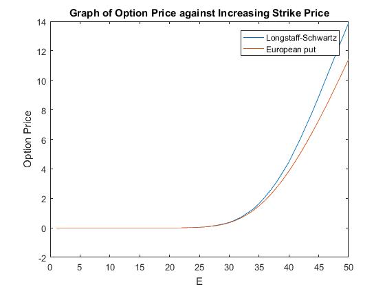
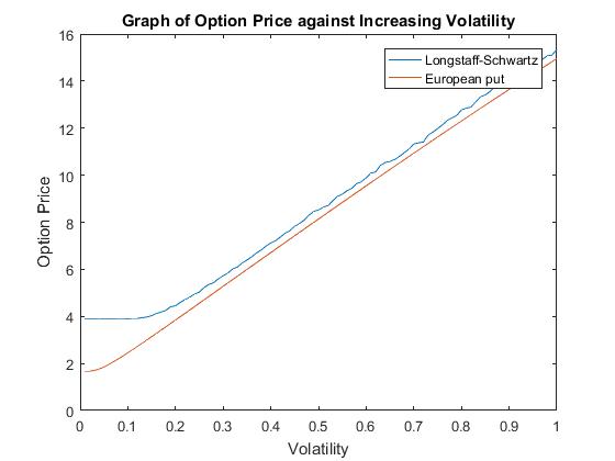
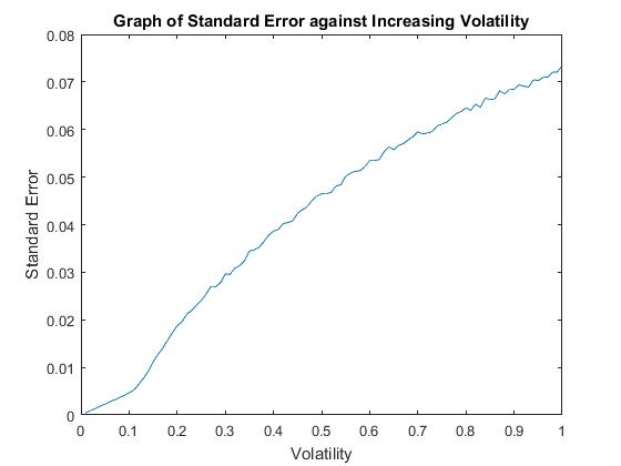
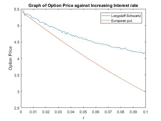
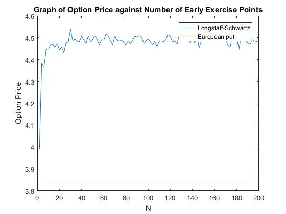
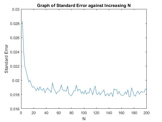
Figure (…)  shows that increasing the number of tie steps which the option can be exercised at has a small effect on the accuracy past a certain point. Once we passed about 40 time-steps the standard error of the method does decline but only by small amounts. This is the reasoning behind why I am only using 50 timesteps in our calculations. Using more timesteps greatly increases the computational time but only slightly improves accuracy.

There are three main sources of error in this method. First, we have the error in the Monte-Carlo method which as

Mincreases approaches 0. Next, we have the error from approximating an American option as a Bermudan option. This approaches 0 as

Nincreases. Finally, we have the error in the estimation of

βiin the regression, again this tends to 0 as the number of basis functions increase. However, increasing these parameters comes at a cost, it increases the computational time exponentially. (Longstaff & Schwartz, 2001) show that only a few basis functions are needed in the regression to achieve accurate results, even in high dimensional problems.

Variance Reduction: Longstaff-Schwartz Algorithm

inputs

M		Longstaff-Schwartz Algorithm	Antithetic Longstaff-Schwartz
10,000	Option Price	4.4993	4.4787
	Standard Error	0.0304	0.01357
	Confidence Interval	4.4986 – 4.4998	4.47846 – 4.47899
	Time (s)	0.0558	1.048
100,000	Option Price	4.4856	4.4873
	Standard Error	0.0091	0.0043
	Confidence Interval	4.485574 – 4.485687	4.48729 – 4.48734
	Time (s)	4.212	8.777

Variance Reduction methods can also be applied to the Longstaff-Schwartz algorithm. Table(…) shows the performance of both the standard Longstaff-Schwartz method and the antithetic sampling version of the Longstaff-Schwartz. Results show that the antithetic sampling greatly reduces the variance of the method. Using 100,000 paths the antithetic sampling reduced the standard error from 0.0091 to 0.0043. The same level of accuracy is achieved using antithetic sampling with 10,000 steps as it is will the standard Longstaff-Schwartz method. Using only 10,000 steps reduces the total computation time for 4.212 to 1.048.

Comparison with the Binomial Method

As previously stated, the binomial method can also be used to find an approximation for the American put price. A slight adaption needs to be made to the algorithm previously stated.

If equation (…) becomes

Vni=MaxPayoffSni,e-rδtpVn+1i+1+1-pVni+1

Then, together with equation (…) and equation (…), we have a method for pricing American options.

Using the same parameter as above, running AmericanBinomial.m yield the following results.

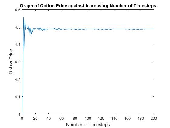
Figure (..) shows a quick convergence to a value of 4.4868 as the number of time-steps increase. This is slightly higher than the 4.478 given by the finite difference method and close the 4.4873. given by the Antithetic Longstaff-Schwartz method. The same saw-tooth behaviour exhibited by the binomial method for the European case is observed here too. It takes roughly 1000 time-steps to converge to 3 decimal places. The program takes 0.04 seconds to run with 1000 timesteps.  The binomial method converges much faster than the Longstaff-Schwartz method. Displaying again that low-dimensional problems are not suitable for Monte-Carlo type methods. The binomial model, however, is ill equipt to deal with higher dimensional problems such as stock prices with jump-diffusions, which the Longstaff-Schwartz method has been shown to do in (Longstaff & Schwartz, 2001)