Dissertation on Detecting Cardiovascular Diseases by Sound

Abstract

Cardiovascular disease (CVD) has always been one of the main causes of death in the world. Accordingly, scientists have been looking for methods to recognize normal/abnormal heart patterns. Over the recent years, researchers have been interested in to investigate CVDs based on heart sounds. The physionet 2016 corpus is presented to provide a standard database for researchers in this field.

In this study we proposed an approach for normal/abnormal heart sound detection, based on i-vector features on phiysionet 2016 corpus. In this method, a fixed length vector, called i-vector, is extracted from each record, and then we applied Principal Component Analysis (PCA) and Linear Discriminant Analysis (LDA) methods to transmission dimension of the obtained i-vector. After that, this i-vector and its PCA and LDA are used for training two Gaussian Mixture Models (GMMs). By these trained GMMs we can reach a score for each test set trial. In the next step we applied a simple global threshold to classify the obtained scores. We reported the results based on Equal Error Rate (EER) and Modified Accuracy (MAcc). Experimental results on the common dataset in the literature show our proposed method could increase the MAcc values about 15.84% compared with the baseline reported results.

1. Introduction

Cardiovascular disease (CVD) is the most common cause of death in most countries of the world and is the leading cause of disability [1].

Reference to the World Heart Association, 2017, 17.7 million people are died every year due to CVDS, which is approximately equal to 31% of all global deaths. The most prevalent CVDs are heart attacks and strokes [1].

In 2013 all 194 members of World Health Organization accepted the implementing Global Action Plan for the Prevention and Control of Non-communicable Diseases, a plan for 2013 to 2020, to be prepared against CVDs. Implementation of nine global and voluntary goals in this plan, the number of premature deaths due to non-communicable diseases is decreased. Among these goals, two of them particularly focus on the prevention and control of CVDs [1].

Accordingly, in recent years, researchers have been interest in to detect heart diseases based on heart sounds. Some related work has been investigated in [2]. Most approaches in this context rely on sound segmentation and feature extraction and machine learning classification on different datasets.

In recent years, various studies have been conducted for normal/abnormal heart sound detection using segmentation methods.

In [3] the Shannon energy envelop for the local spectrum is calculated by a new method, which uses S-transform for every sound produced by heart sound signal. Sensitivity and positive predictively was evaluated on 80 heart sound recording (including 40 normal and 40 pathological), and their values were reported over 95%.  In a study by [4] an approach proposed for automatic segmentation, using Hilbert transform. Features for this study included envelops near the peaks of S1, S2, the transmission points T12 from S1 to S2, and visa-versa. Database for this study, consisted of 7730s of heart sound from pathological patients, 600s from normal subjects, and finally 1496.8 s from Michigan MHSDB database. Average accuracy for sound with mixed S1, and S2, was 96.69%, and for those with separated S1 and S2, it was reported 97.37%. Another envelope extraction method engaged for heart sound segmentation is called Cardiac Sound Characteristic Waveform (CSCW). The work presented in [5] used this method for only a small set of heart sounds, including 9 sound recording and the accuracy was reported 99.0%. No train-test split was performed for evaluation in this study.

The work in [6] achieved an accuracy of 92.4% for S1 and 93.5% for S2 segmentation by engaging homomorphic filtering and HMM, on PASCAL database [7]. The work investigated in [8] also used the same approach with wavelet analysis on the same database and accuracy for S1 was reported 90.9% for S1 segmentation and this value was 93.3% for S2 segmentation. There is also a study on expected duration of heart sound using HMM and Hidden Semi-Markov Model (HSMM) introduced in [9]. In this study, positions of S1 and S2 sounds was labeled in 113 recording, first. After that they calculated Gaussian distributions for the expected duration of each four states including S1, systole, S2 and diastole, using average duration of mentioned sound and also autocorrelation analysis of systolic and diastolic durations. Homomorphic envelope plus three other frequencies features (in 25-50, 50-100 and 100-150 Hz ranges) were among features they used for this study. Then they calculated Gaussian distributions for training HMM states and emission probabilities. Finally, for decoding process, backward and forward Viterbi algorithm engaged and they reported 98.8% sensitivity and 98.6% positive predictively. This work also proposed HSMM alongside logistic regression (for emission probability estimation) to accurately segment noisy, and real-world heart sound recording [10]. This work also used Viterbi algorithm to decode state sequences. For evaluation, they used a database of 10172s of heart sounds recoded from 112 patients. F1 score for this study reported 95.63%, improving the previous state of the art study with 86.28% on same test set.

Other works were also developed using other methods based on the feature extraction and classification using machine learning classifier such as ANN, SVM, HMM and kNN.

For distinction between spectral energy between normal and pathological recordings, the work introduced in [11] extracted five frequency bands and their spectral energy was given as input to ANN. Results on a dataset with 50 recorded sounds showed 95% sensitivity and 93.33% specificity.

In a study by [12], a discrete wavelet transform in addition to a fuzzy logic was used for a three-class problem; including normal, pulmonary stenosis, and mitral stenosis. An ANN was employed to classify dataset of 120 subjects with 50/50 split for train and test set. Reported results was 100% for sensitivity, 95.24% for specificity, and 98.33% for average accuracy. Moreover, he used time-frequency as an input for ANN in [13]. This work reported 90.48% sensitivity, 97.44% specificity, and 95% accuracy on same dataset for same problem (three-class classification including normal, pulmonary and mitral stenosis heart valve diseases).

The work in [14] also performed a study to classify normal and pathological cases using Least Square Support Vector Machine (LSSVM) engaging wavelet to extract features. They evaluated their method on a dataset with heart sound of 64 patients (32 cases for train and 32 cases for test set) and reported 86.72% accuracy. In a work [15] with same classifier, used wavelet packets and extracted features like sample entropy and energy fraction as input. Dataset used for this problem consisted of 40 normal persons and 67 pathological patients and they resulted 97.17% accuracy, 93.48% sensitivity and 98.55% specificity. In another study [16], also used LSSVM as classifier while using tunable-Q wavelet transform as input features. Evaluation in this study showed 98.8% sensitivity and 99.3% specificity on a dataset comprising 4628 cycles from 163 heart sound recordings, with unknown number of patients. As another work on SVM [17], engaged frequency power with varying length frames over systole as input features, and used Growing Time SVM (GTSVM) for classifying pathological and normal murmurs. Results on 56 persons (including 26 murmurs and 30 normal) was reported 86.4% for sensitivity and 89.3% for specificity.   Another work on HMM was performed by [18] where a HMM was fit to the frequency spectrum form heart cycle and used four HMMs for evaluating posterior probability of the features given to model for classification. For better results, they used Principal Component Analysis (PCA) as reduction procedure and results were reported 95% sensitivity, 98.8% specificity and 97.5% accuracy on a dataset with 60 samples.

As an approach for clustering, the work in [19] employed K-Nearest Neighbor (K-NN) on a features obtained from various time-frequency representation extracted from subset of 22 persons including 16 normal persons and 6 pathological patients. They reported 98% accuracy for this problem where likelihood of over-training was used as parameters for KNN. The work investigated in [20] also chose K-NN for clustering the samples as normal and pathological. This study also employed two approach for dimensionality reduction of extracted time-frequency features; linear decomposition and tiling partition of mentioned features plane. Results were achieved on totally 45 recordings; including 19 pathological and 26 normal, and they was reported as 99.0% average accuracy with 11-fold cross-validation.

In the following, to organize these studies and due to the lack of standard dataset in this context, the PhysioNet/CinC Challenge 2016 and its related database is introduced [2]. This database has been collected from a total of 9 independent databases with different numbers and types of patients and different recording quality, over a decade. Some of the related works on PhysioNet 2016 are investigated below:

Table 1. Summary of the previous heart sound works, methods, database and results [2].

Acc%	P+%	Sp%	Se%	Method	Database	Author
–	95	–	96/97	Segmentation	–	Moukadem et al (2013)
96.69	–	–	–	Segmentation	–	Sun et al (2014)
99.0	–	–	–	Segmentation	–	Yan et al (2010)
92.4/93.5	–	–	–	Segmentation	PASCAL	Sedighian et al (2014)
90.9/93.3	–	–	–	Segmentation	PASCAL	Castro et al (2013)
–	98.6	–	98.8	Segmentation	–	Schmidt et al (2010a)
–	–	93.3	95	Frequency + ANN	36 normal and 54 pathological	Sepehri et al (2008)
95	–	97.44	90.48	Time-frequency + ANN	40 normal, 40 pulmonary and 40 mitral steno	Uguz (2012b)
86.72	–	–	–	Wavelet + SVM	64 patients (normal and pathological)	Ari et al (2010)
98.9	–	99.3	98.8	Wavelet + SVM	40 normal and 67 pathological	Zheng et al (2015)
–	–	89.3	86.4	Frequency + SVM	30 normal, 26 innocent and 30 AS	Gharehbaghi et al (2015)
97.5	–	98.8	95	DFT and PCA + HMM	40 normal, 40 pulmonary and 40 mitral stenosis	Saracoglu (2012)
98	–	–	–	Time-frequency + kNN	16 normal and 6 pathological	Quiceno-Manrique et al (2010)
99	–	98.54	99.56	Time-frequency + kNN	16 normal and 6 pathological	Avendano-Valencia et al (2010)
–	–	78.91	77.49	mRMR + SVM	Physionet 2016	Puri et al (2016)
84.90	–	86.91	85.90	Time-frequency + ANN	Physionet 2016	Zabihi et al (2016)
–	–	77.8	94.24	Time-frequency and AdaBoost + CNN	Physionet 2016	Potes et al (2016)
88	–	100	75	MFCC + CNN	Physionet 2016	Rubin et al (2016)

The work presented in [21] employed a feature set of 54 total features extracted from timing information for heart sounds, using mutual information and based Redundancy Maximum Relevance (mRMR) technique and also usednon-linear radial basis function based Support Vector Machine (SVM) as classifier. In this work, 0.7749% Sensitivity and 0.7891% Specificity was reported on the hidden test set.

In the work investigated in [22], the time, frequency, and time-frequency domains features are employed without any segmentation. To classify these features, an ensemble of 20 feedforward ANN used for classification task and achieved overall score of 91.50% (94.23% for sensitivity and 88.76% for specificity) on train set and 85.90% (86.91% sensitivity and 84.90% specificity) on blind test setThe work presented in [23] reports 0.9424 Sensitivity, 0.7781 Specificity and overall score 0.8602 on blind data set using total of 124 time-frequency features and applying variant of the AdaBoost and convolutional neural network (CNN) classifiers.

The work [24] employed CNN method for classification of normal and abnormal heart sounds based on the MFCC features. The experimental results was reported in two phases according to different applying train set. The sensitivity, specificity and overall scores on hidden set for the phase one was 75%, 100% and 88%, respectively. Also, for the phase two sensitivity, specificity and overall scores on hidden set was reported 76.5%, 93.1% and 84.8%, respectively. Table 1 summarizes the works investigated in this section.

In this study, we focus on detect heart diseases using heart sounds based on the PhysioNet/CinC Challenge 2016 and we aim to provide an approach rely on identity vector (i-vector).

Although the i-vector was originally used for speaker recognition applications [25], it is currently used in various fields such as language identification [26] [27], accent identification [28], gender recognition, age estimation, emotion recognition [29] [30], audio scene classification [31] etc. In this study, we adopt the i-vector to normal/abnormal heart sound detection.

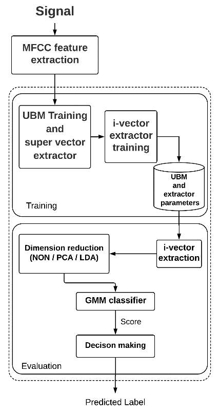
Figure 1: Block diagram of MFCC feature extraction [26].

Our motivation for using this method in this context is owing to the fact that human heart sounds can be considered as physiological traits of a person [32] which are distinctive and permanent, unless accidents, illnesses, genetic defects, or aging have altered or destroyed them [32].

In this work, we utilized two features, Comprising Mel-Frequency Cepstral Coefficients (MFCCs) and i-vector and also we used Gaussian Mixture Models (GMMs) as classifier. To detect a normal heart sound signal from the abnormal we extracted the MFCCs features from the given heart sound signal, and then we obtained the i-vector of each heart sound signal using MFCCs.

Furthermore, to classify a normal heart sound form abnormal, we trained GMMs and then applied the i-vecors to them. The rest of this paper is organized as follows: in Section 2 features and classifier are introduced. The experiment setup is and experimental results are reported in Section 3 and 4, respectively. Eventually, the conclusion is presented in Section 5.

2. Features and Classifiers

2.1 mel-frequency cepstral coefficients

MFCCs were engaged over years as one of the most important features for speaker recognition [33]. The MFCC attempts to model the human hearing perceptions by focusing on low frequencies (0-1Khz) [34]. In better words, the differences of critical bandwidth in human ear is basis of what we know as MFCCs. In addition, Mel frequency scale is applied to extract critical features of speech, specially its pitch.

2.1.1 MFCC Extraction

In the following, we will explain how the MFCC feature is extracted. Initially, the given signal s[n] is pre-emphasized. The concept of “pre-emphasis” means the reinforcement of high-frequency components passed by a high-pass filter [33]. The output of the filter is as follows:

pn=sn-0.97s[n-1] (1)

In the next step, the pre-emphasized signal is divided into short-time frames (e.g. 20ms) and Hamming windows are pre-processed. The hamming windows can be applied as:

hn=pn ×0.54-0.46cos⁡2πnN-1   0≤n

1 (2)

Where N is number of samples in each frame.

To analyze h[n] in the frequency domain, a N-point Fast Fourier Transform (FFT) is applied to convert them into the frequency. The frequency of the FFT can be computed according to:

Hk=∑n=0N-1hne-j2πnN (3)

A logarithmic power spectrum is obtained on a Mel-scale using a filter bank consists of L filter:

Xl=log⁡∑k=kllkluHk Wlk    l=0,1,…,L-1 (4)

Where Wlk is the lth triangular filter, kll and klu are the lower limit and upper limit of the lth filter, respectively.

The given frequency f in herttz can be converted to Mel-scale as follows:

FMel=[2595 ×log⁡101+f 700] (5)

Eventually, the MFCCs coefficients are obtained by applying Discrete Cosine Transform (DCT) to the

Xl:

Cm= ∑l=1LXlcos⁡πml-0.5L       m=1,…, M-1 (6)

Where m is the obtained features form frequency components of Xl. The steps for extracting the MFCC are depicted in Fig. 1.

2.2 i-Vector

Currently i-vector in total variability space has become the state-of-the-art approach for speaker recognition [25]. This method that was introduced after its predecessor method, joint factor analysis [35] [36], can be considered as a technique to extract a compact fixed-length representation given a signal with arbitrary length. Then, the extracted compact feature vector can be either used for vector distance-based similarity measuring or as input to any further feature transform or modelling. There are certain steps to extract i-vector from a signal. First, features (e.g. MFCC) should be extracted from the input signal and then the Baum–Welch statistics should be extracted from the features [37], and finally i-vector is computed using these statistics. In the following, we explain these steps in details.

2.2.1 Universal background model (UBM) training

The first step in i-vector extraction pipeline is to create a global model which is called an UBM [38]. For UBM, various models are used based on the application. Usually, GMM is used for this purpose in text-independent speaker verification [25] [39] and HMM is used in text-dependent applications [40] [41] [42]. In normal/abnormal heart sound detection tasks, we train a GMM from all the extracted features of all individuals in the development set. There should be sufficient training data in the development set for this model to properly cover the feature space. A GMM is a weighted set of C multivariate Gaussian distributions and formulated as:

Prxλ= ∑c=1Cwc Nxmc,∑c (7)

where x is a D-dimensional vector with continuous values, w shows the weight for each component of the mixture, and Nxmc,∑c shows the Gaussian distribution with mean mc and covariance matrix ∑c. The sum of all weights should be equal to one. Usually, GMM is used with a diagonal covariance matrix in practise and we use a diagonal matrix in this study too [43].

2.2.2 Extraction of Baum–Welch statistics

In this step, for each feature sequence, the zero and first-order Baum–Welch statistics are computed using the UBM [44] [45].

Given Xi as the entire collection of feature vectors for training record ith, the zero, and first-order statistics (i.e. Nc and Fc) for the cth component of the UBM are computed as follows:

NCXi= ∑tγi,tc (8)

FCXi= ∑tγi,tc(Xi,t-mc) (9)

where Xi, t shows the tth vector of entire features for record ith, mc is the mean of cth component, and γi,tc is the posterior probability of generating Xi, t by the cth component as follows:

γi,tc=Pr⁡cXi,t=wc Nxmc,∑c∑j=1Cwj NXi,tmj,∑j (10)

2.2.3 i-Vector

Let M show the individual dependent mean-supervector that represents the feature vectors of a record. The term supervector is referred to the DC-dimensional vector obtained by concatenating the D-dimensional mean vectors of the GMM corresponding to a given record (it can be obtained by classical maximum a posteriori (MAP) adaptation [46]). In the i-vector method [25], this supervector is modelled as follows:

M=m+Tw (11)

where m is an individual independent mean-supervector derived from the UBM, T is a low rank matrix, and w is a random latent variable having a standard normal distribution. The i-vector ϕ is the MAP point estimate of the variable w which is equal to the mean of the posterior probability of w given the input record. In this setting, it is assumed that supervector M has a Gaussian distribution with mean m and covariance matrix TTt.

2.2.4 Training the parameters of the model

In (5 = previous equation), m and T are the parameters of the model. Usually, the mean supervector of the UBM is used as m. This supervector is formed by concatenating the means of the UBM components [48]. To train T, the expectation maximisation (EM) algorithm is used [37]. Let the UBM have C components and the dimensions of feature vectors be D. First, the matrix Σ is formed as follows:

∑=∑100∑2⋯00⋮⋱⋮00⋯∑C (12)

where ∑c is the covariance matrix of the cth component of the UBM. Assuming Xi shows the entire collection of feature vectors for record ith and P(Xi| Mi, Σ) denotes the likelihood of Xi calculated with the GMM specified by the supervector Mi and the super-covariance matrix Σ, then the EM optimisation is done by repeating the following two steps:

1. For each training records, we use the current value of T and compute the vector that maximises the likelihood in the following way:

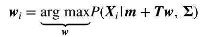  (13)

2. Then we update T by maximising the following equation:

∏iPXim+Twi,  ∑ (14)

By taking the logarithm of (14), the product is replaced with summation and also the likelihood is replaced with log-likelihood which can be calculated for each record using the following equation:

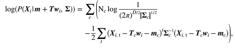(15)

where c iterates over all components of the model and t iterates over all feature vectors. Tc is a submatrix of T related to the cth component. Assuming we have computed the zero and first-order statistics using (8) and (9), we can compute the posterior covariance matrix [i.e.

Cov(wi, wi)], mean (i.e.

E[wi]) and the second moment (i.e.

E[wiwit]) for

wi using the following relations:

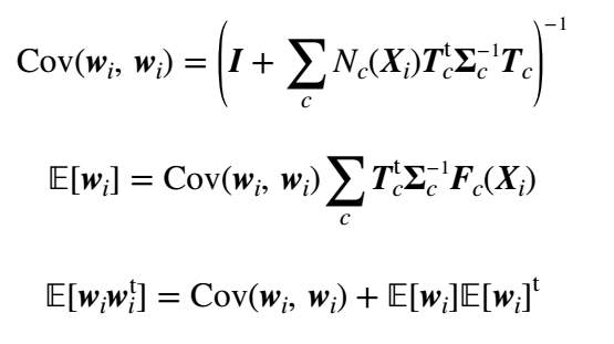(16) (17) (18)

Finally, if we maximise (20), the following relation is obtained for updating matrix T:

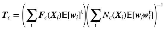(19)

2.2.5 Computing the i-vector

As explained in the previous section, w is a random hidden variable with standard normal distribution, where i-vector is the mean of the posterior probability of w given the input record. To find i-vector, the MAP point estimation of w is used and the formula is the same as (17).

2.2.6 Methods for extract important information and reducing the effects of intra-class variations

Several methods have been proposed for extract important information and reducing the effects of intra-class (within class) variations. For i-vector-based method, the widely used such methods are nuisance attribute projection (NAP) [25] [48] [49] [50], within-class covariance normalization (WCCN) [25] [51] [52], principal component analysis (PCA) [reference] and linear discriminant analysis (LDA) [25]. Here, we used PCA and LDA which will be explained in the following section.

2.2.6.1 PCA

In this method, important information is extracted from the data as new orthogonal variables, which are referred to as the principal components [53].

To achieve this, assume a given n ×pzero mean data matrix X(n and p indicate the number of experiment repetition and a particular feature, respectively). Accordingly, to define the transformation consider vector x(i) of X which is mapped by a set of p-dimensional vectors of weights w(k)=(w1,…,wp)(k) to a new vector of principal component t(i)=(t1,…,tl)i, as follows:

tk(i)= xi . w(k) ;  i=1,…,n    k=1,…,l (20)

In other words, vector t (consists t1,…,tl ) inherit the maximum variance from x by weight vector w constrained to be a unit vector [54].

2.2.6.2 LDA

The LDA and PCA methods are very structurally similar and both try to minimize variance of data, but LDA also try to maximize intra-class variance to improve separation [56].

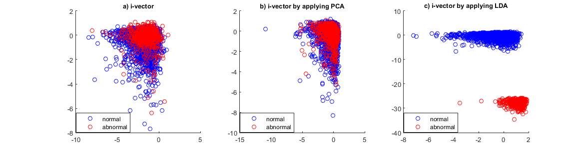
Fig 2. Two first dimensions of 64-dimensional i-vector extracted from physionet 2016 training set and effect of PCA and LDA on it.

So, if we consider a sample with x⃗ representation (e.g. feature vector) and label equal to y, our goal is to predict label for class y, given a sample of a distribution with vector x⃗ observation.[56].

LDA assumes a two class problem and consider conditional density functions with px⃗y= 0 and px⃗y= 1 normally distributed and with mean and covariance parameter equal to (μ0⃗,Σ0) and (μ1⃗,Σ1). Considering these situation, a sample belongs to second class based on bayes optimal solution, if likelihood ratio is higher than Threshold T. So that [57]:

  (21)

As a result, final classifier can be called a quadratic discriminant analysis (QDA).

LDA also assumes that class covariance is identical, and in addition they have full rank. Hence, several terms are ignored.[57]:

x⃗T∑0-1x⃗=x⃗T∑1-1x⃗ (22)

and the above decision criterion becomes a threshold on the dot product:

w⃗.x⃗ >c (23)

For a constant c we have:

w⃗= ∑-1(μ1⃗-μ0⃗)  (24)

c= 12(T-μ0⃗T∑-1μ0⃗+μ1⃗T∑-1μ1⃗) (25)

As a result we can say considering input

x⃗ in a class with label y, is a direct linear combination of observations. There is a geometrical description for this criteria: considering x⃗ in a class with label y is a direct function of multidimensional projection from x⃗ to vector w⃗. In better words, the observation x⃗ has y label if its projection on a certain side of hyperplane is w⃗ vector. This location is determined by value c.

Fig. 2 shows the effect of these PCA and LDA on the i-vector. Fig. 2a shows two first dimensions of the 64-dimensional i-vectors extracted from the physionet/CinC 2016 training data in which the MFCCs were used as features. And fig. 2b,c show the 64-dimensions i-vector reduced into 2-dimensions by PCA and LDA, respectively.

2.3 Gaussian Mixture Models

In this work, Gaussian mixture models (GMMs) are used as classifier. GMMs are probabilistic models used to represent normalized distributions of a sub-population in a general population. In general, GMMs let the model automatically learn its sub-population without having to know which sub-population belongs to a given data point. Since sub-population allocation is not known, this kind of learning is known as un-supervised learning.

2.3.1 Gaussian model

The GMM is introduced with two types of values: the weights of the Gaussian mixture components and the means and the variance of the Gaussian mixture components. The probability distribution function (PDF) of a K components GMM, with mean μ⃗k and covariance matrix ∑k for the kth component is defined as:

px⃗= ∑i=1K12πK∑iφiexp⁡(-12x⃗-μi⃗T∑i-1x⃗-μi⃗) (26)

∑i=1kφi=1 (27)

Table 2. Statistics of the 2016 PhysioNet/CinC dataset [2].

Subset	# patients	# Recordings	# Proportion of recordings (%)   Abnormal    Normal       Unsure			# The weight parameters   wa1            wa2             wn1            wn2
Training   Eval. Test.	764   – 308	3153   301 1277	18.1   – 12.1	73.03   – 77.1	8.8   – 10.9	0.8602   0.78881 –	0.1398   0.2119 –	0.9252   0.9467 –	0.0748   0.0533 –

Where

x⃗ is a feature vector and φk is the weight of the mixture components.

2.3.2 Learning the model

2.3.3 Maximumlikelihood estimation of GMMs

Maximizing Likelihood estimation of Gaussian mixture models includes two steps. The first step is known as “exaptation”, which includes calculating the exaptation and assigning the kth component (Ck) for each xiϵX data point with the parameters of the model φk, μ⃗k and ∑k. The second step is known as “maximization”, which includes maximizing the expectation calculated in the previous step relative to the model parameters. This step involves updating the values of φk, μ⃗k and ∑k.

The entire process is repeated as long as the algorithm converges, and it gives maximum likelihood estimation. More details are available at [58].

3. Experimental Setup

3.1. Dataset

The 2016 PhysioNet/CinC challenge is introduced to provide a standard database containing normal and abnormal heart sound [2]. The presented dataset in this challenge is a heart sound recordings set of subjects/patients which is collected from variety of environmental conditions (including noisy conditions with low signal quality) as described in [reference]. Therefore, many heart sounds have been incurred different noises during recordings such as speech, stethoscope motion, breathing and intestinal activity. These noises make difficult to classify normal and abnormal heart sounds. Accordingly, the organizers allowed the participants to classify some of the recordings as ‘unsure’ [2] and it shows the difficulty level of the challenge. This corpus consists three subsets: training, validation and test. For training purposes, six labeled databases (names with prefix a to f) containing 3153 sound recording from 764 subjects/patients, with duration of 5-120 s).

The validation subset is comprised of 150 normal and 151 abnormal heart sound (with file names prefixed alphabetically, a through e.) and the test data includes 1277 hearts sound trials generated from 308 subjects/patients. It is necessary to mention that 301 selected recording from train set used as test set for validation.

The Challenge test consisted of six databases labeled from b to e, g, and i with 1277 heart sound recordings from 308 subjects.

It should be noted that the test set is unavailable to the public and will remain private for the purpose of scoring. The statistics of each subset are summarized and illustrated in Table 2. More details about the corpus and the 2016 PhysioNet/CinC challenge can be found in [2].

In this work, we reported our results based on physionet/CinC 2016 dataset. It is worth mentioning that validation subset is consisted of 301 records, which is a copy of the training data. Accordingly, in order to report valid results, we first removed the validation records from the training set and then divided the training set into two parts in five phases. In each phase, we randomly assigned 80% of training set as our training set and the rest of 20% were assigned as our validation set which is used for tuning the parameters. In addition, we used physionet/CinC 2016 validation set as our test set.

3.2 Evaluation Metrics

In this task the metric of evaluation is reported based on Equal Error Rate (EER) and Modified Accuracy (MAcc). Therefore, to compute EER, we assign to each trial a score value, then let define Pfa(θ) as the false alarm and

Pmiss(θ) as the miss rates at threshold θ: (28)

Pfaθ=#{abnormal trials with scores > θ}#{Total abnormal trials} (29)

Pmissθ=#{normal trials with scores ≤ θ}#{Total normal trials}

Now EER is computed [4]:

EER= Pfa(θEER)=PmissθEER (30)

where θEER is the value of the parameter θ when Pfa equals Pmiss.

Also for MAcc computation, classified data are in three class; normal, abnormal or unsure, with two references in each categories. The modified sensitivity (Se) and specificity (Sp) can be computed according to:

Se= wa1 × Aa1Aa1+Aq1+An1+ wa1 × (Aa2+Aq2)Aa2+Aq2+An2 (31)

Se= wn1 × Na1Na1+Nq1+Nn1+ wn1 × (Na2+Nq2)Na2+Nq2+Nn2 (32)

where wa1 and wa2 are the percentages of the abnormal recordings of the signal with good quality and poor quality respectively, and  wn1 and wn2 are of the normal recordings of the signal with good quality and poor quality respectively.

For all 3153 training set recordings, values for weight parameters of wa1, wa2, wn1 and wn2 are equal to 0.8602, 0.1398, 0.9252 and 0.0748 respectively, in train set. These parameters also calculated for validation set and they were reported 0.78881, 0.2119, 0.9467 and 0.0533 respectively. The “Score” for this challenge is computed using following equation:

MAcc=(Sp+Se)/2 (33)

3.3 Proposed Method

The proposed method aims at using the i-vector for normal/abnormal heart sound detection. In this method, we first train a GMM using all heart sounds (i.e. both normal and abnormal heart sounds) in our training set. After training this UBM, we use it to extract zero and first-order statistics of the training features. Then, using these statistics we train an i-vector extractor using several iterations of the EM algorithm explained in Section 2.3.2. After training the i-vector extractor, we extract i-vectors from all records in our training set. In this stage, we have extracted several i-vectors with different dimensions for each record in the training set and we use them to train the intra-class variation reduction methods.

Specifically, we train LDA transforms from the original heart sounds in our training set and use them to transform the i-vectors to the new space. After training the required. transforms, we extract i-vectors from the heart sounds and transform them using PCA and LDA. Therefore, we have a representative i-vector for each record, which we will use for scoring.

3.4 Scoring and decision making

To assign score to a given heart sound based on GMM classifier we proceed as follows. First, we extract an i-vector from our training set and project them to the new space using the PCA or LDA and apply them to two GMMs (one GMM for the normal heart sound and the other for the abnormal heart sound) with different components to learn the model by EM iterations (training GMMs). In the next step, the score for each trial is obtained by computing log likelihood ratio:

LLRS=logPSθ not mal-logPSθ abnormal (34)

where S is a feature vector corresponding to the test record and θ normal and θ abnormal denote the GMMs for normal and abnormal heart sound, respectively. After finding the score, a simple global threshold is applied to it to make the final decision of normal/abnormal heart sound detection. If the score was higher than the threshold, the test heart sound is labeled as normal and otherwise it is labeled as abnormal. In this paper, we used a global threshold to be able to plot the detection error tradeoff (DET) and detection accuracy tradeoff (DAT) curves. Fig. 3 illustrates our proposed system.

Figure 3: Our proposed system structure.

MAcc%

Sp%

Se%

EER%

MAcc%

Sp%

Se%

EER%

MAcc%

Sp%

Se%

EER%

Dimensions with applying PCA/LDA

i-vector dimensions

88.05

83.4

92.66

12.22

91.03

88.07

94

9.1

88.3

91.3

85.3

12

W.A

64

91.7/92.69

89.4/91.39

94/94

10.01/7.55

93/94

94.7/94.7

91.3/93.3

7.2/5.9

87.65/88.35

92.7/88.7

82.6/88

12.4/11.8

16

91/88.3

90/90

92/86.6

8.8/7.06

92/93.3

92.71/93.3

91.3/93.3

8.1/6.5

89.66/89.35

94.03/90.7

85.3/88

10.1/11.05

32

88.05/91.02

84.1/92.05

92/90

11.8/8.33

91.35/94.33

89.4/93.37

93.3/95.3

8.7/6.15

89.69/88.66

92.05/90

87.33/87.33

10.21/11.3

64

89.37

86.09

90.66

11.07

91.7

88.74

94.66

8.38

85.37

86.75

84

14.72

W.A

128

93/95.01

89.4/96.02

96.6/94

7.23/5.91

93.01/95.01

95.36/95.36

90.66/4.66

7.41/5.64

88.35/90.3

92.71/91.39

84/89.3

11.8/10.2

16

91.03/95.01

88.74/95.36

93.33/94.66

10.85/5.75

93.67/95.01

96.02/96.02

91.33/94

6.11/5.88

91.66/91.68

94.03/93.37

89.3/90

8.35/9.15

32

90.70/93.68

87.41/94.7

94/92.66

10.49/6.18

93.69/94.35

90.72/92.71

96.66/96

6.16/5.23

91.01/91.68

92.71/93.37

89.33/90

9/8.48

64

88.73

80.13

97.33

11.30

89.02

90.72

87.33

10.81

87.02

92.05

82

12.55

W.A

256

92.37/95.65

88.74/94.7

96/96.6

7.81/5.59

92.65/94.01

947.7/94.03

90.6.3/94

7.53/6.48

88.34/91.02

96.68/91.39

80/90.66

12.7/8.33

16

93/95.3

89.4/96.6

96.6/94

7.66/5.36

93.34/95.35

94.03/94.7

92.66/96

7.40/5.14

89.98/94.34

93.37/94.03

86.6/94.66

12.23/8.76

32

90.7/95.95

85.4/96.6

96/95.3

10.5/4.77

92.03/96.01

90.06/94.70

94/97.33

8.38/4.1

89.01/94.68

93.37/94.7

84.66/94.66

10.28/9/4

64

90.37

86.09

94.66

11.68

92.03

88.74

95.33

8.42

89.35

92.71

86

11.65

W.A

512

92.36/91.37

89.40/87.41

95.33/95.33

8.29/8.53

95.01/94.68

96.02/94.70

94/94.66

5.87/5.23

89.68/93.34

92.71/94.03

86.66/92.66

12.2/6.83

16

91.37/95.34

88.74/95.36

94/95.33

9.14/5.31

94.34/95.34

95.35/95.36

93.33/95.33

5.5/4.63

91.68/94.68

93.37/94.70

90/94.66

10.25/9.66

32

86.39/93.35

81.45/92.71

91.33/94

14.02/8.66

92.01/94.68

90.72/94.70

93.33/94.66

8.87/5.1

91.02/93.35

92.71/93.37

89.33/93.33

8.83/6.44

64

86.06

78.8

93.33

13.77

89.04

86.09

92

10.34

81.38

84.1

78.66

18.92

W.A

1024

95.98/96.98

93.37/97.3

98.6/96.67

5.79/4.81

95/97.05

98.67/96.68

91.3/97.33

5.44/2.80

87.68/96.34

94.7/96.68

80.66/96

12.30/3.46

16

93.37/97

87.41/98.67

99.33/95.33

7.74/3.12

94.33/97.34

98.01/96.02

90.66/98.86

6.18/2.95

89.67/97

96.02/98.68

83.33/97.33

9.59/3.08

32

91.05/96.97

83.44/97.35

98.66/96.6

8.84/3.55

93.7/97.33

88.74/98.67

96.66/96

6.3/2.80

89.36/97.34

91.39/97.35

87.33/97.33

11.98/2.71

64

Table 3. EER and MAcc comparison based on UBM components count, raw i-vector dimension and dimension of i-vector using PCA and LDA for the proposed method. Here the word “W.A” means “Without Applying PCA or LDA”.

4. Experimental Results

In this section, first we briefly introduce the baseline system and in the following we introduce the experimental results which include two parts. In the first part we investigate the effect of GMM components and i-vector dimensionality using whole of training set. In the second part we were interested in investigating the effect of applying different sizes of training set to our proposed system.

4.1 Baseline system

In this paper we consider the work presented in [] as the baseline system. The physionet 2016 dataset is used in the baseline system in the same way that we used in our system. The proposed method in the baseline system is based on asynchronous frames []. Accordingly, 103228 frames were extracted from physionet 2016 dataset. To report the results, they repeated their experiments five times and reported the average of obtained results. The attained results in terms of sensitivity, specificity and mean accuracy was reported 0.845, 0.785 and 0.815, respectively.

4.2 Effects of GMM components count and i-vectors dimensionality

First part of our experiments were performed to investigate the effects of the number of GMM components, the dimension of i-vectors Without Applying (W.A) LDA and PCA and dimension reduction by applying PCA and LDA. Table 3 represents the obtained EERs and sensitivities and specificities by our different systems on the test set.  It is worth mentioning that we did not label any data as “unsure”, and we assigned “normal” or “abnormal” labels to all test data. Furthermore, in this part we applied whole of training set to our system.

In each element of Table 3, there are two result values (separated by a slash) that represent the effect of using the PCA and LDA techniques. In addition, the number of components used in GMMs are specified separately in the table.

Table 3 shows i-vector and its LDA performs better than others (right side of slash). As shown in this table, the best results are achieved by higher dimensions of i-vector and its LDA.

The left side of slash denotes the results of i-vector and its PCA. It is observed that the result values obtained by applying PCA are not as good as of applying LDA values are. This is due to the fact that LDA operates supervised, however PCA operates unsupervised.

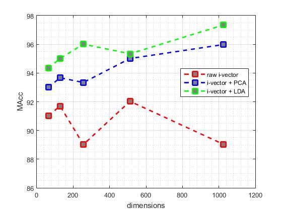
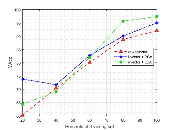
Fig. 4 and fig. 5 illustrate the best EER and MAcc values achieved by our proposed systems from test data, respectively. The red point-line of fig. 4 and fig. 5 represent the best values achieved by different dimensions of i-vectors without applying PCA or LDA. Also, blue point-line and green point-line of the fig. 4 and fig. 5 represent the best values obtained by different dimensions of i-vectors and applying PCA and LDA, respectively.

As shown n the Fig 4 and Fig 5, commonly the EER values decrease with increasing dimensions of the i-vectors and applying LDA or PCA to them, an the MAcc values increase, subsequently. But this pattern is not true for i-vectors without applying LDA or PCA, and they are given different EER and MAcc values.

Fig. 4 DET curve comparison for raw i-vevtor and its PCA and LDA. In each case, results are reported using the best parameters configuration.

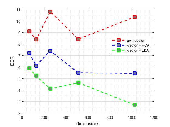
Fig. 5 DAT curve comparison for raw i-vevtor and its PCA and LDA. In each case, results are reported using the best parameters configuration

Discussion

A higher-dimensional i-vector includes more detailed information. On the other hand, this information should be meaningful. Therefore, the PCA and LDA methods are used to make this information meaningful. As shown in Table 3,  applying PCA and LDA can significantly improve the result values relative to the applying raw i-vectors. Among them, due to the fact that LDA working supervised and it is learned by considering test data labels, consequently has a better performance than PCA in dimension transmission of test data and meaningful of the obtained details from i-vector data. Therefore we can see that better result values are obtained by increasing the i-vector dimensions.

As it is described in Table 3, generally the best EER values and MAcc values are obtained by the GMMs which are trained by 128 components.

Table 4 shows the results obtained by the baseline system and the best results obtained by our proposed systems in this paper. Accordingly, the best accuracy achieved by our proposed system is 97.34% that could improve the accuracy of the baseline system by 15.84%.

Table 4. Comparison the best results obtained by our proposed systems and the results of the baseline system.

System	EER %	Se %	Sp %	MAcc %
baseline	–	84.5	78.5	81.5
i-vector   i-vector + PCA i-vector +LDA	8.38   5.44 2.71	88.74   93.37 96.02	95.33   98.6 98.86	92.03   95.98 97.34

4.3 Effect of training the system using different size of training set

In second part of our experiments we are going to evaluate the effect of different size of training set on proposed method. To reach this goal, we divided the training data into 5 parts (each part include 20% of training set) randomly. In the next step, we add one of these parts each time to the previous part to see the impact of increasing training set on the proposed system. Table 5 shows the effect of applying different size of training set to our system, in which the number of GMM components were fixed at 128, which obtained the best results in the first part of our experiments. The values reported in this table are based on the best results obtained from the different size of raw i-vectors and applying PCA and LDA to them. (In each case, results are reported using the best parameters configuration).

As it is summarised in Table 5, the classification performance is improved by increasing the amount of training data.

The results suggest that increasing the size of training data beyond 80% leads to less improvement, when compared to the cases where size of the training set are smaller.

According to Table 5, our proposed system performed similar to the baseline system when only 60% of training set is used.

Table 5. The Effect of Using Different Size of training set on the performance of the Proposed System

Size of training set	System	EER%	Se %	Sp %	MAcc%
20%	Raw i-vector   i-vector + PCA i-vector +LDA	37.85   30.12 31.31	86.00   95.33 40.00	34.44   52.32 88.74	60.22   73.82 64.37
40%	Raw i-vector   i-vector + PCA i-vector +LDA	24.75   27.44 28.95	66.00   60.00 65.33	74.83   83.44 72.85	70.41   71.72 69.09
60%	Raw i-vector   i-vector + PCA i-vector +LDA	20.38   17.82 18.95	65.33   82.00 64.67	94.7   83.44 99.34	80.10   82.70 82.00
80%	Raw i-vector   i-vector + PCA i-vector +LDA	11.94   8.27 4.12	89.33   88.00 93.33	87.42   92.05 98.01	88.75   90.02 95.67
100%	Raw i-vector   i-vector + PCA i-vector +LDA	8.38   5.44 2.80	88.74   91.30 96.02	95.33   98.67 98.86	92.03   95.00 97.34

Fig. 6 and Fig. 7 show the classification MAcc and EER of the proposed system as a function of training set size. Fig. 6 and Fig. 7 depict the effect of varying training set size on the EER and MAcc values, respectively.

Fig. 6 DET curve comparison for raw i-vevtor and its PCA and LDA for using different size of training set. In each case, results are reported using the best parameters configuration

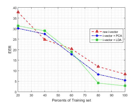
Fig. 7 DAT curve comparison for raw i-vevtor and its PCA and LDA for using different size of training set. In each case, results are reported using the best parameters configuration

5. Conclusions

This paper proposes a novel method for automatic heart sound classification based on i-vector MFCC feature embedding, in which MFCC is extracted from heart sounds to represent the characteristics of the subject’s heard sound. The experiments on a public dataset demonstrate the effectiveness of the proposed method.

This method is based on fix-sized i-vector and therefore insensitive to the length of the input sounds. Combination of MFCC and i-vector are stable and can reflect the key point features to discriminate two types of subject accurately. The i-vector feature of heart sound is more suitable to describe the characteristics of heart sound than other length variable features since the sound is always regarded as a whole when producing the i-vector.

The proposed method has low computational cost and can work well on even wearable devices and it also works well even when the amount of training data is little. In conclusion, the proposed method outperforms the state-of-the-art approaches.

References

[1] E. J. e. a. Benjamin, “Heart disease and stroke statistics-2017 update: a report from the American Heart Association,” pp. e146-e603, 2017.

[2] C. e. a. Liu, “An open access database for the evaluation of heart sound algorithms,” 2016.

[3] A. e. a. Moukadem, “Localization of heart sounds based on S-transform and radial basis function neural network.,” 15th Nordic-Baltic Conference on Biomedical Engineering and Medical Physics (NBC 2011). Springer, pp. 168-171, 2011.

[4] S. e. a. Sun, “Automatic moment segmentation and peak detection analysis of heart sound pattern via short-time modified Hilbert transform.,” Computer methods and programs in biomedicine 114.3, pp. 219-230, 2014.

[5] Z. e. a. Yan, “The moment segmentation analysis of heart sound pattern.,” Computer methods and programs in biomedicine 98.2, pp. 140-150, 2010.

[6] P. e. a. Sedighian, “Pediatric heart sound segmentation using Hidden Markov Model.,” Engineering in Medicine and Biology Society (EMBC), 2014 36th Annual International Conference of the IEEE. , p. 5490–5493, 2014.

[7] B. e. al, “The PASCAL classifying heart sounds challenge 2011 (CHSC2011) (www.peterjbentley.com/heartchallenge/index.html),” 2011.

[8] A. e. a. Castro, “Heart sound segmentation of pediatric auscultations using wavelet analysis,” Engineering in Medicine and Biology Society (EMBC), 2013 35th Annual International Conference of the IEEE, 2013.

[9] S. E. e. a. Schmidt, “Segmentation of heart sound recordings by a duration-dependent hidden Markov model.,” Physiological measurement 31.4 , pp. 513-529, 2010.

[10] S. e. al., “Logistic regression-hsmm-based heart sound segmentation,” IEEE Transactions on Biomedical Engineering 63.4, pp. 822-832, 2016.

[11] A. A. e. a. Sepehri, “Computerized screening of children congenital heart diseases.,” Computer methods and programs in biomedicine 92.2 , pp. 186-192, 2008.

[12] H. Uğuz, “Adaptive neuro-fuzzy inference system for diagnosis of the heart valve diseases using wavelet transform with entropy,” Neural Computing and applications 21.7, pp. 1617-1628, 2010.

[13] H. Uğuz, “A biomedical system based on artificial neural network and principal component analysis for diagnosis of the heart valve diseases.,” Journal of medical systems 36.1 , pp. 61-72, 2012.

[14] A. e. al., “Detection of cardiac abnormality from PCG signal using LMS based least square SVM classifier.,” Expert Systems with Applications 37.12 , pp. 8019-8026, 2010.

[15] Z. e. al., “A novel hybrid energy fraction and entropy-based approach for systolic heart murmurs identification.,” Expert Systems with Applications 42.5 , pp. 2710-2721, 2015.

[16] P. e. al., “Automatic diagnosis of septal defects based on tunable-Q wavelet transform of cardiac sound signals,” Expert Systems with Applications, pp. 3315-3326, 2015.

[17] A. e. a. Gharehbaghi, “Assessment of aortic valve stenosis severity using intelligent phonocardiography.,” International journal of cardiology 198, pp. 58-60, 2015.

[18] R. SaraçOğLu, “Hidden Markov model-based classification of heart valve disease with PCA for dimension reduction,” Engineering Applications of Artificial Intelligence 25.7, pp. 1523-1528, 2012.

[19] A. F. e. a. Quiceno-Manrique, “Selection of dynamic features based on time–frequency representations for heart murmur detection from phonocardiographic signals.,” Annals of biomedical engineering 38.1, pp. 118-137, 2010.

[20] L. D. e. a. Avendano-Valencia, “Feature extraction from parametric time–frequency representations for heart murmur detection,” Annals of Biomedical Engineering 38.8, pp. 2716-2732, 2010.

[21] C. e. a. Puri, “Classification of normal and abnormal heart sound recordings through robust feature selection,” Computing in Cardiology Conference (CinC), 2016, pp. 1125-1128, 2016.

[22] M. e. a. Zabihi, “Heart sound anomaly and quality detection using ensemble of neural networks without segmentation,” Computing in Cardiology Conference (CinC), 2016, pp. 613-616, 2016.

[23] C. e. a. Potes, “Ensemble of feature-based and deep learning-based classifiers for detection of abnormal heart sounds,” Computing in Cardiology Conference (CinC), 2016, pp. 621-624, 2016.

[24] J. e. a. Rubin, “Classifying heart sound recordings using deep convolutional neural networks and mel-frequency cepstral coefficients,” Computing in Cardiology Conference (CinC), 2016., pp. 813-816, 2016.

[25] N. K. P. D. R. e. a. Dehak, “Front-end factor analysis for speaker verification,” IEEE Trans. Audio Speech Lang. Process., 2011, 19, (4), pp. 788-798, 2011.

[26] N. T.-C. P. R. D. e. a. Dehak, “Language recognition via i-vectors and dimensionality reduction’,” InterSpeech, pp. 857-860, 2011.

[27] D. P. O. B. L. e. a. Martınez, “Language recognition in i-vectors space,” Interspeech, pp. 861-864, 2011.

[28] M. S. R. V. L. D. e. a. Bahari, “Accent recognition using i-vector, Gaussian mean supervector and Gaussian posterior probability supervector for spontaneous telephone speech,” IEEE Int. Conf. Acoustics Speech and Signal Processing (ICASSP), p. 7344–7348, 2013.

[29] R. L. Y. Xia, “Using i-vector space model for emotion recognition,” Interspeech, 2012.

[30] H. E. E. Khaki, “Continuous emotion tracking using total variability space,” InterSpeech, 2015.

[31] H. L. B. D. M. e. a. Eghbal-zadeh, “CP-JKU submissions for DCASE-2016 : a hybrid approach using binaural i-vectors and deep convolutional neural networks,” 2016.

[32] M. R. e. a. Hasan, “Speaker identification using mel frequency cepstral coefficients,” 3rd International Conference on Electrical &ComputerEngineering ICECE, Dhaka, Bangladesh, pp. 565-568, 2004.

[33] R. e. a. Wahid, “”A Gaussian mixture models approach to human heart signal verification using different feature extraction algorithms.,” Computer Applications for Bio-technology, Multimedia, and Ubiquitous City, pp. 16-24, 2012.

[34] V. Tiwari, “MFCC and its applications in speaker recognition,” nternational journal on emerging technologies 1.1, pp. 19-22, 2010.

[35] L. M. B. a. I. E. Muda, “Voice recognition algorithms using mel frequency cepstral coefficient (MFCC) and dynamic time warping (DTW) techniques.,” arXiv preprint arXiv:1003.4083, 2010.

[36] J. e. a. Jo, “Energy-Efficient floating-point MFCC extraction,” IEEE Transactions on Very Large Scale Integration (VLSI), pp. 754-758, 2016.

[37] P. e. a. Kenny, “Joint factor analysis versus eigenchannels in speaker recognition,” IEEE Transactions on Audio, Speech, and Language Processing 15.4, vol. 1447, p. 1435, 2007.

[38] P. e. a. Kenny, “A study of interspeaker variability in speaker verification.,” IEEE Trans. Audio Speech Lang. Process., pp. 980-988, 2008.

[39] P. e. a. Kenny, “Eigenvoice modeling with sparse training data,” IEEE transactions on speech and audio processing 13.3, pp. 345-354, 2005.

[40] D. Q. T. D. R. Reynolds, “Speaker verification using adapted Gaussian mixture models,” Digit. Signal Process., 2000, 10, (1), pp. 19-41, 2000.

[41] H. M. A. S. H. e. a. Zeinali, “Non-speaker information reduction from cosine similarity scoring in i-vector based speaker verification,” Comput.Electr. Eng., 2015, 48, pp. 226-238, 2015.

[42] H. K. E. S. H. e. a. Zeinali, “Telephony text-prompted speaker verification using i-vector representation,” IEEE Int. Conf. Acoustics Speech and Signal Processing (ICASSP), pp. 4839-4843, 2015.

[43] H. S. H. B. L. e. a. Zeinali, “-vector/HMM based text-dependent speaker verification system for RedDots challenge,” InterSpeech, pp. 440-444, 2016.

[44] H. S. H. B. Č. e. a. Zeinali, “Text-dependent speaker verification based on i-vectors, deep neural networks and hidden Markov models,” Comput. Speech Lang., pp. 53-71, 2017.

[45] D. Q. T. D. R. Reynolds, “Speaker verification using adapted Gaussian mixture models,” Digit. Signal Process., 2000, 10, (1), pp. 19-41, 2000.

[46] P. O. P. D. N. e. a. Kenny, “A study of interspeaker variability in speaker verification,” IEEE Trans. Audio Speech Lang. Process., pp. 980-988, 2008.

[47] P. B. G. D. P. Kenny, “Eigenvoice modeling with sparse training data,” IEEE Trans. Speech Audio Process., p. 345–354, 2005.

[48] D. A. T. F. Q. a. R. B. D. Reynolds, “Speaker verification using adapted Gaussian mixture models,” Digital signal processing 10.1-3 , pp. 19-41, 2000.

[49] W. S. D. R. D. e. a. Campbell, “SVM based speaker verification using a GMM supervector kernel and NAP variability compensation,” IEEE Int. Conf. Acoustics, Speech and Signal Processing (ICASSP), pp. 97-100, 2006.

[50] A. C. Q. a. W. M. C. Solomonoff, “Channel compensation for SVM speaker recognition.,” Odyssey– The Speaker and Language, vol. 4, pp. 219-226, 2004.

[51] A. C. W. B. I. Solomonoff, “Advances in channel compensation for SVM speaker recognition,” IEEE Int. Conf. Acoustics,Speech and Signal Processing (ICASSP), pp. 629-632, 2005.

[52] A. K. S. S. A. Hatch, “Within-class covariance normalization for SVM-based speaker recognition,” InterSpeech, p. 1874, 2006.

[53] N. K. P. D. R. e. a. Dehak, “Support vector machines and joint factor analysis for speaker verification,” IEEE Int. Conf. Acoustics, Speech and Signal Processing (ICASSP), p. 42374240, 2009.

[54] H. a. L. J. W. Abdi, “Principal component analysis,” Wiley interdisciplinary reviews: computational statistics 2.4, pp. 433-459, 2010.

[55] D. H. P. a. G. C. Jang, “Estimation of leakage ratio using principal component analysis and artificial neural network in water distribution systems.,” Sustainability 10.3 , p. 750, 2018.

[56] C. R. Rao, “The utilization of multiple measurements in problems of biological,” Journal of the Royal Statistical Society. Series B (Methodological) 10.2 , pp. 159-203, 1948.

[57] W. N. a. B. D. R. Venables, “Random and mixed effects,” Modern applied statistics with S. Springer,New York, NY, pp. 271-300, 2002.

[58] A. e. a. Tharwat, “Linear discriminant analysis: A detailed tutorial.,” AI Communications 30.2, 169-190.

[59] D. A. Reynolds, “Automatic speaker recognition using Gaussian mixture speaker models.,” the Lincoln Laboratory Journal, pp. 173-192, 1995.