An Artificial Neural Network Approach for Detecting Spectrum Sensing Data Falsification Attacks

Abstract

In spectrum sensing data falsification attacks, malicious users send falsified reports to either the fusion center or to other users to deceive them about the availability of frequency channels, well-known as. Failing to detect these attacks can have severe consequences on the performance of cognitive radio networks. In the past decade, a handful techniques have been proposed to detect these attacks using either statistical or machine learning based approaches. The statistical approaches perform well under specific settings, but they are inefficient in detecting sophisticated and well-crafted attacks. In addition, the delay of the detection of statistical-based approaches is high, which is not practical for on-fly detection.

The existing machine learning approaches, on the other hand, have a low detection performance as their probability of detection drops with an increase of both the probabilities of miss-detection and false alarm under low values of signal-to-noise-ratio or under dense attacks. Therefore, there is a strong need for proficient mechanisms to detect spectrum sensing data falsification attacks under intense attacks within acceptable delays.

In this paper, we propose a multi-layer neural network classifier to detect falsified reports in cooperative spectrum sensing. A rigorous methodology is used to train, evaluate, and test the model. The energy statistic of the received samples, the signal-to-noise ratio, and the distance between the primary user signal and secondary users are the feature used for this classification. Several experiments were conducted to optimize the structure of the neural network. The obtained results show that with a structure of two hidden layers of 20 neurons each, the proposed model can achieve a probability of detection as high as 90.4% and a probability of false alarm as less as 8% with an accuracy of 98.5%.

Index Terms — cognitive radio, cooperative spectrum sensing, spectrum sensing data falsification attacks, machine-learning, k-means clustering, neural network, logistic regression, support vector machine, cross-validation, probability of detection, probability of false alarm, probability of miss-detection, accuracy.

I. INTRODUCTION

The internet of things is taking over enabling many applications such as, but not limited to autonomous vehicles, smart healthcare, virtual reality, smart homes, and smart cities, all of which have contributed to the dramatic growth in wireless communications by which a shortage in the radio spectrum has been created [1]. Billions of wireless devices are going to demand high-speed Internet access, which can be translated into higher demands for bandwidth making the static management of the radio resource,  no longer efficient to grant access to all these devices and meet their increasing demands for higher bandwidth [2].

In addition, the free propagation channels of radio transmission makes wireless communications intrinsically at risk of being target to several security breaches such as denial of service attacks, specially-crafted attacks, and interferences –whether accidentally due to implementation imperfections, or intentionally due to malicious intent to abuse the spectrum, all of which reduce the spectrum efficiency. To circumvent this shortage in the radio spectrum, there is a strong need for mechanisms that increase the efficiency of spectrum sharing among the multitude of users, cognitive radio technology [3].

Cognitive radio technology, simply put, is a smart wireless solution that enables dynamic and fair radio spectrum access sharing among multitude of users to increase the spectrum efficiency by which unlicensed users, secondary users, are authorized to dynamically access any free frequency channel without causing any harmful interference to licensed users, primary users [4]. There are two foundational process upon which cognitive radio technology rests. One is spectrum sensing, in which the secondary users sense the activity of the primary user. The other one is spectrum decision, in which secondary users decide upon the results of spectrum sensing, which channels are free and which ones are occupied [3]. Thus, the way forward to increase the spectral efficiency is to enable cognitive radio network [5]. Cognitive radio has undergone extensive investigation in the past decade and as a result, several novel spectrum sensing techniques have been proposed to enable dynamic spectrum access [6].

Examples of these techniques include energy detection [7–9], cyclostationary detection[10–12], and matched filter detection [13–15]. The detection performance of these techniques is often compromised with fading effects, shadowing, and other types of losses [16]. To mitigate these effects, secondary users often cooperate to correctly detect the availability of the frequency channels through the exploitation of the spatial diversity. In this cooperative spectrum sensing, several secondary users cooperate by sharing their local sensing decisions to detect the state of the primary user’s signal accurately [16]. This cooperation can be either centralized [17,18] or decentralized [19] .

In the centralized cooperation, the secondary users perform spectrum sensing and send their local sensing decisions to a central entity, called fusion center, which combines these decisions to obtain the final decision using fusion rules such as the “OR”, “AND”, or “K-out-of-N” rules [20] or soft combining [21]. In the decentralized cooperation, distributed spectrum sensing, there is no central entity such as the fusion center, but each secondary user reports and receives reports from its neighbors’ and takes the final decision on its own. Most of the previous cooperative sensing techniques are neither robust nor resilient to malicious and specially-crafted attacks that abuse the radio spectrum [25][26]. Examples of these attacks include the primary user emulation [27,28], jamming attacks [29,30], and spectrum sensing data falsification attacks [31].

In the first type of attacks, malicious users mimic the primary user’s signal to prevent other users from using frequency channels. In the second type of attacks, malicious users send continuous or intermittent signals to flood the control channel and prevent secondary users from communicating either between then or with the fusion center, and thereby creating distributed denial of service. In the third type of attacks, main focus of this research paper, malicious users report falsified local sensing decisions about the availability of the radio spectrum to their neighbors or the fusion center. If the frequency channel is free, the malicious users report that this channel is occupied to prevent the secondary users from accessing it; while if this channel is occupied, the malicious users report that the channel is free to enable secondary users to access the channel thereby causing harmful interference to the primary user.

Failling to cope with these attacks can result in abuse of the radio spectrum. Therfore, the task facing the designers of cognitive radio communication systems is that of increasing the resilience of these networks to these attacks. Researcher’s in cognitive radio networks were focus on designing reliable spectrum sensing and were careless about the security aspect of these networks, and consider it as separate task. However, curretly, researcher’s come to realize that this way of approaching security always give the attackers one step ahead. Thus, they are aiming at making cyber security an intrinsic characteristic of these networks[3,32]. And this can be seen in the growing interest in developing secure and reliable spectrum sensing mechanisms in the presence of malicious users [31].

As a result, several detection techniques have been proposed to cope with spectrum sensing data falsification attacks [33–35] [36–45] [46–51] [52–60] [61–63]. These techniques can be classified into two main classes: statistical-based and machine-learning-based. Methods of the first class use statistical models to detect falsified reports while methods of the second class use machine-learning classifiers such as support vector machine and logistic regression to classify users as honest or malicious. Methods of the first class, as the authors of [31] suggested, can be grouped into several categories, global-based, mean-based, or distribution-based. Methods of the first category are global decision-based [36–45], in which the fusion center discard the users whose local decisions contradict the global decision. These global decision-based techniques are simple and easy to implement. However, they are not effective in detecting attacks when the number of malicious users is high because the fusion center can eliminate honest users instead of malicious ones, which makes the fusion center broadcast the wrong decisions about the availability of frequency channels. Techniques under the second category are mean-based [46–51].

In these techniques, the mean value of the reports is used as a reference to determine falsified reports, which consist of outliers with significant deviation from the mean. These outliers are assumed to be falsified reports and the fusion center discard them from the process of the fusion to take the final decision. Techniques under this category are simple and with high robustness, but ineffective in the case of a high number of attackers. The methods of the third category are distribution-based [52–60], in which the sensing reports are assumed to underline a probability distribution and the falsified reports are expected to deviate from this distribution. These techniques have been proven to be effective in eliminating malicious users, but they suffer high computation and long delay detections. Methods of the last category, utility-based [61–63], assume that the attackers, in this case, have utilities to maximize, and they are guided to send accurate reports through punishments or rewards according to their objectives. However, in most of the cases, the attackers are irrational and unpredictable, and their goals can be limited to disturbing the communication.

Techniques of the first class work well under specific setting, but in general, they are ineffective to detect spectrum sensing data falsification attacks in real-time since the delay of classification is very high. Techniques of the second class are machine learning (ML) based techniques. As shown in Table I, unsupervised and supervised machine learning techniques have been proposed using several features to distinguish trusted users from malicious ones. For instance, the authors of [64,65] suggested an unsupervised machine learning method based on k-means clustering to classify users into two classes trusted users and malicious ones. This technique uses the historical sensing information as a feature to classify users, trusted or malicious. It starts by initializing of the centroid of the two clusters, and then, it attributes each user to one of these two classes that minimizes the identification errors of each measurement and the centroids.

This approach can be efficient in distinguishing malicious users from trusted ones; however, this technique is known for its sensitivity to the initial centroids as different initializations could lead to different results. The authors did not evaluate the impact of this initialization on the classification accuracy. The authors of [66] suggested the use of a supervised machine learning algorithm, Bayesian learning, to discard falsified reports in cooperative sensing. Each user has attribute weights that reflects its trustworthiness. All users start with an initial weight equal to 1, and each user has attributed a prior distribution. The fusion center updates the poster distribution and decreases a user’s weights if the received sensing report does not match the global decision. This technique is proficient in detecting malicious users with high probability. However, the use of the global decision as a reference can be the weakness of the model in the sense that if the global decision corresponds to the wrong decision, the model can be trained with false training dataset.

Furthermore, the authors did not provide any information about the training size, and they did not show the learning curves to see if the model is not suffering from the problem of overfitting as no cross-validation technique was used. The authors of [67] proposed an algorithm, called support a vector data description (SVDD), to detect malicious users in cooperative sensing. This technique was able to classify nodes into malicious users and trusted one. However, the probabilities of detection and false alarm are highly dependent on the number of attackers in the sensing, and if this number is higher than 20, the probability of detection drops to 50% and the probability of false alarm increases to reach 100%.

The authors of  [68] proposed an unsupervised machine learning technique based on artificial neural network, self-organizing map (SOM), in which the average suspicion degree (ASD) is used to classify the nodes into malicious and trusted users. The reported results show that the model performs well under good values of signal-to-noise ratio (SNR), but the performance drops dramatically under a high level of noise as the probability of miss-detection exceeds 50% at low values of SNR.

TABLE I. Related Work of SSDF detection using Machine Learning Techniques

	Features	Advantages	Limitations
k-means clustering [64,65]	Energy statistic	No training data is required Simple approach Short delay of detection Evaluation using probabilities of detection and false alarm	Sensitivity to the sensing history dimension High computational cost with large sensing history Decreased rightness of classification with small history dimension. Sensitivity to the initialization of the centroid Probability of detection, miss-detection are dependent on the level of SNR
Bayesian learning [66]	Energy statistic	The size of training data is increased with each classification The nodes are not discarded completely from the fusion Evaluation using both the probability of detection and false alarm	Dependency to the correctness of the global decision Computational costly No information about the training and testing sizes is given No cross-validation technique is considered No learning curves are provided Probability of detection, miss -detection are dependent on the level of SNR
SVDD [67]	Energy statistic	High detection performance under small size of the attacks population	Heuristic approach  Low detection performance under high intensity of attacks The performance of the technique is dependent on the level of SNR
SOM [68]	Average suspicion degree (ASD)	Good detection performance under high signal-to-noise ratio Evaluation using probabilities of detection and false alarm	Probability of detection, miss-detection, and false are dependent on the level of SNR  Low detection performance under low values of signal-to-noise ratio

The theory of machine learning can be proficient in distinguishing malicious users from trusted ones within an acceptable delay for real-time detection, especially, with a better selection of the features and following a rigorous methodology to train, evaluate, and test the model [69]. The wireless environment is time-varying and the attackers often change their strategy over time and from one user to another. The use of simple approaches, which are often characterized by their limiting rigidity, they stays unchanged and fail to detect sophisticated and specially-crafted attacks.

Machine learning, in which the behavior adapts to its input data – solves such issues; they are, by nature, adaptive to changes in the wireless environment they interact with. In addition, large and complex datasets can be easily recorded. These datasets are treasures of meaningful information which are way too large and too complex for humans to make sense of. Machine Learning is a promising tool to detect meaningful patterns in large and complex data sets. In this research paper, we propose a supervised machine learning algorithm approach to detect malicious users in cooperative spectrum sensing using a Neural Network based approach.

Features such as the energy statistic, the received signal-to-noise ratio, and the distance between the primary user and secondary users are used to train the model. To use these features, we assume that the nodes send their received samples to the fusion center as well as the level of the signal-to-noise ratio measured by a technique based on the eigenvalues of the covariance matrix of the received samples. Also, we assume that the fusion center keeps track of the position of the secondary users as well as the primary user position. The structure of our neural network is optimized in a way to maximize the probability of detection of the malicious nodes while decreasing the probability of false alarm. The performance of the algorithm is evaluated and compared to those of other existing techniques using metrics such as the probability of detection, the probability of false alarm, and accuracy. The main contributions of this paper can be summarized as follows:

• A mathematical model of spectrum sensing data falsification attacks
• A feature set for identifying attackers
• Generation of large representative dataset
• Validation of the proposed model with experimental results using several metrics
• Comparison of the proposed model with existing techniques such as support vector machine and logistic regression

The rest of this paper is structured as follows. Section II describes the mathematical model of cooperative spectrum sensing, the attack model, features used, and the methodology used to train the machine learning technique as well as the mathematical model of multi-layer neural network technique. Section III presents the simulation details, describes the dataset generation, and also presents and discusses the obtained results. Conclusions and perspectives are drawn in section IV.

II. Methodology

This section herein deals with describing our methodology, and it is divided into two parts: The first part describes the mathematical of cooperative spectrum sensing and the spectrum sensing data falsification attack model as well as features used. The second parts of this section, describes how neural network have been applied in the context of cooperative spectrum sensing to detect falsified reports and discard them. Specifically, we express the cross-entropy cost function as a function of the features and we solve the optimization problem to detect the optimal weights corresponding to each features. These process as well as some other details are given in this part.

A. spectrum sensing data falsification model and features description

As shown in Fig. 1, we consider a set of N secondary users performing spectrum sensing to detect the availability of a frequency channel f. These secondary users report their collected samples to the fusion center and measure their level of signal-to-noise ratio using a technique based on the eigenvalues of the covariance matrix of the received samples. In addition, the fusion center is assumed to know the location of the primary user as well as the secondary users at each time.

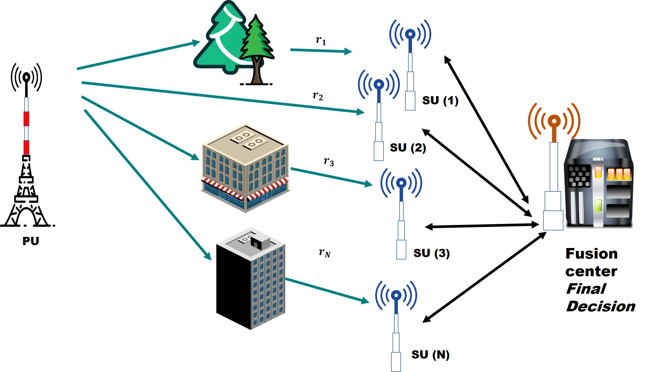
Fig. 1. Cooperative spectrum sensing scenario in which several SUs report the sensing information to the fusion center that combines these local decisions to determine the availability of frequency channels [].

The fusion center combines the reports and decides between two channel’s states HO, the primary user is absent, and H1, the primary user is absent.

H0: xn=w(n)	(1)
H1: xn=s(n)+w(n)	(2)

where x is the received signal, wis the noise, and sis the primary user’s signal. The primary users signal is considered to be a signal with a transmission power Pt. The secondary users are distributed in a geographic area with random distance from the primary user’s signal. The reported samples by the ithsecondary users at a time slot tis given by:

xi,t=hij*rssi,t*δi+n0,t+ei,t,         i= 1, 2,…, n

(3)

Where hij, denotes the channel model between the ith secondary user and the fusion center, n0,tis a Gaussian noise, and ei,tis the injected samples by the attacker, if iththe secondary users is honest, this parameter should be null; otherwise, this parameter can takes two possible values. If the δi=0, the attacker injects a value of ei,t>threhold, and if δi=0, the attacker injects a value of ei,t≤threshold. The rssi,tis given by the following equation:

rssi,t=10log⁡PtGtGr2πdi,t2+20log⁡(λ)

(4)

where di,t is the distance between the primary users and the i thsecondary user at the time slot t, Pt is the transmission power of the primary user signal, and λ  is the wave length, Gr is the receiver antenna gain, and Gtis the primary user transmitter’s antenna gain. The energy statistic is squared magnitude of the fast Fourier transform of the received signal averaged over the number of samples collected. It is given by:

Energy Statistic=1N∑n=1NXi,t[n]2

(5)

where N is the total number of received samples at the time slot t, Xi,tis the Fast Fourier transform of the received samples xi,t. The use of the energy statistic as a feature to detect falsified reports is not enough. Indeed, the received samples are often corrupted by the noise, and if the signal of an honest user has a low value of signal-to-noise ratio, this user can report that the primary user signal is absent as the energy detector perform poorly under low signal-to-noise ratio. In this case, the fusion center is going to discard honest users, which may degrade the overall detection performance of the network. To remedy to this issue, we propose to use, in addition to the energy statistic, the signal-to-noise ratio at each secondary user. Each secondary user can measure the signal-to-noise ratio based on the eigenvalues of the sample covariance matrix of the received samples [70,71]. In the following, the mathematical model of this technique is described. The received signal, ri,t, can be expressed as an N×Lmatrix, whose entries are as follows:

ri,t=(ri,t)1,1⋯(ri,t)1,N⋮⋱⋮(ri,t)L,1⋯(ri,t)L,N

(6)

where (rssi,t)i, j is the (i,j)th component of the vector of the received signal samples at the level of the ithsecondary user at the time slot t. The noise and the signal are assumed to be independent, and the noise is considered to be additive white Gaussian noise components with mean 0 and variance σW2. Therefore, for each secondary user, Equations (1) and (2) can be rewritten as:

H0: ri,tn=wi,t(n)	(7)
H1: ri,tn=st(n)+wi,t(n)	(8)

where ri,t is the received signal component at the ithsecondary user at the time slot t, stis the transmitted component in the time slot t, and wiis the noise component. Given an observation bandwidth B, a transmitted signal with occupied bandwidth bin the sample covariance matrix eigenvalues domain, and u≤L, uL  denotes the fraction of the whole observation bandwidth occupied by the transmitted signal. The rest of the bandwidth is the occupied by noise. When L,N→∞, the statistical covariance matrices of the noise, of the transmitted samples, and of the received samples are defined as:

Rwi,t=Ewi,tn*wi,tHn=σW2.IL ; -∞	(9)
Rst=Estn*stH(n)	(10)
Rri,t=Eri,tn*ri,tH(n)	(11)

where Rwi,t denotes the noise statistical covariance matrix, Rst denotes the transmitted signal statistical covariance matrix, Rri,t denotes the received signal statistical covariance matrix, (.)H denotes the complex conjugate transpose, σW2denotes the noise variance, and ILdenotes the L-order identity matrix. Since the signal and the noise are independent, we have the following equation,

Rri,t=Rst+Rwi,t=Rst+σW2.IL

(12)

Given the eigenvalues λri,t of Rri,t and λst of Rst in a descending order, we get,

(λri,t)j=Rri,t+σW2,    ∀j=1,2…u	(13)
(λst)j=σW2 ∀j=u+1,u+2, …L	(14)

where is the group of eigenvalues The statistical covariance matrix eigenvalues are equal to signal components power. Thus, the estimate of the received statistical covariance matrix Rx̂can be calculated instead of statistical covariance matrix as there exists a finite number of samples. The sample covariance matrix of the received signal is given by:

R̂ri,t=1Nri,tri,tH

(15)

The eigenvalues of the samples covariance matrix deviate from the signal power components following Marcenko Pastuer probability density function, which depends on the value of LN. The value of uis estimated using the Minimum Descriptive Length criterion. The estimated value of u, denoted as û, is given by:

U=argminu⁡-L-UNlog⁡φUθU+12U2L-Ulog⁡N;0≤u≤L-1

(16)

where

φu=∏j=u+1Lλj1L-u	(17)
θu=1L-u∑j=u+1Lλj	(18)

where L denotes the number of eigenvalues, N denotes the number of samples, and λidenotes the set of eigenvalues. After estimating the value of u, the signal group of eigenvalues is determined as λ1… λuand the noise group eigenvalues as λu+1…λL. To compute the noise variance σW2, two values σW12and σW22are calculated as follows:

σW12=λL(1-c)2	(19)
σW22=λû+1(1+c)2	(20)

K linearly spaced values in the range [ σW12, σW22] are denoted as πk,where 1≤k≤K. The Marcenko Pastuer density of parameters c, σw, is given by:

mpc,σw=dFWV=(v-σW21-c2)(σW21+c2-v)2πσW2vcdv

(21)

where v is bounded by σW21-c2and σW21+c2

σW21-c2≤v≤σW21+c2

(22)

Using Eq. 21, we can calculate K Marcenko Pastuer densities of the parameters (1-β̂)cand πk where β̂=ûL and the empirical distribution function (EDF) of the noise group eigenvalues is given by,

EDF=Fnt=number of samples values≤tn

(23)

where n is the total number of sample values in the noise eigenvalues. The noise eigenvalues empirical distribution is then compared with the Marcenko Pastuer densities and a goodness of fitting is used to pick the best estimate of in order to fitting and is given by:

GDπk=EDF-mp((1-β̂c, πk))2

(24)

The estimate of the noise variance, σW2̂, is given by:

σW2̂ = minπk⁡(GD(πk))

(25)

Once the noise power has been estimated, the signal power can be calculated as the difference between the total power of the received samples and the estimated noise power. The power of the collected samples is given by:

snr̂=rssi,tσW2̂=10log⁡PtGtGr2πdi,t2+20log⁡(λ)minπk⁡(GD(πk))

(26)

Table II summarizes the features used to train the neural network classifier, which are the energy statistic, the estimated signal to noise ratio, and the distance between the primary user and each secondary user. A description of these features is also given in this table as well as a reference for the equations used to estimate each feature.

TABLE II. Features used to train the neural network

Features	Description
Energy Statistic	The energy of the received samples or the test statistic, it is given by the sum of the FFT of the received samples squared over the number of samples, it is given by Eq. 5
Signal-to-noise Ratio	The estimated noise ratio at the level of each SNR based on the eigenvalues of the covariance matrix of the received samples. Its estimate is given by Eq. 26
Distance	The distance between the secondary user and the primary user signal. It is obtained from the Eq. 4

B. Neural Network

Machine learning algorithms can be classified into two main categories: supervised and unsupervised machine learning [69]. In contrast to unsupervised machine learning, supervised techniques use some training dataset to train the model so that it can predict the output of a new test data. One of the most reliable classifiers is the neural network classifier. Imitating the behavior of an artificial functional model from the biological neuron. The neural network is composed of at least three parts: the input layer, one or more hidden layers, and the output layer. The input layer is formed by the input’s features used to train the neural network model. The hidden layers, each one consisting of one or more neuron, learn the abstract representations of the inputs. The output layer implements the network classification, and because the model is a binary classification, this output has only one neuron.

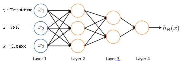
Fig 2. Neural Network consisting of one input layer with three features, two hidden layers, and one output layer

Each neuron is composed of an activation function g. The output of each neuron is the activation function of the sum of all the weighted input values ∑i=nwixi and the bias b, which can be expressed as:

g=g(∑i=nwixi+b)

(27)

where g is the activation function. The most known examples of activation functions used in neural networks include but not limited to the sigmoid, hyperbolic tangent, and the relu functions. The forward propagation is an essential concept used in neural networks, which consists of taking each input value from the input layer and multiplying it by the weight of each connection between the units and neurons, then summing up the products of all connections to the neurons. The activation function of this sum is then calculated in each neuron. This operation is repeated for all neurons in all hidden layers until we get to the output layer. In the following, we describe the mathematical model of forward propagation. The input features are given as follows:

x=[x0, x1,x2,…,xm]=a(0)

(28)

Where m is the number of the inputs features. Herein m=3 and x0is the energy statistic, x1is the signal-to-noise-ratio at the level of each secondary user, and x2is the distance between the primary user and each secondary user. The following equation gives the output of the first neuron of the first hidden layer:

a1(2)=g12(∑i=1mw1i1xi+b1i1)

(29)

where g12 is the activation function of the first hidden layer and the layer, xi is the ith  layer input value, w1i1 is the weights corresponding to the connection between the ith  layer input value and the first neuron of the first hidden layer, and b1i1 is the bias corresponding to the first neuron in the first hidden layer. In general, the ithneuron of the lth  layer is given by:

aj(l)=gjl(∑i=1mwjilail-1+bjil)

(30)

The output layer of a neural network consists of one neuron with an activation function ggives the hypothesis function as follows:

hwx=g(∑i=1mwi(l)ail)

(31)

We previously described the forward propagation, in the following, we describe how neural networks learn their weights and biases using gradient descent algorithm, this process is known as backpropagation. Given a training set x(1),y(1),x(2),y(2),…,x(m),y(m), the cross-entropy cost function J(W), or the cross-entropy error function tells us how the cost or the error changes when we change the weights and the bias. It is equivalent to minus log-likelihood for the data y(i) under the hypothesis hwx. The mathematical expression of this cost function is given by:

JW=-1m∑im∑k=1Kyk(i)log⁡hw(x(i))k+(1-yk(i))log⁡(1-hw(x(i))k)+λ2m∑l=1L-1∑i=1sl∑j=1sl+1(wj,i(l))2

(32)

where λ is the regularization parameter, m is the training data size, K  is the number of the output classes, which is 2 in this methodology, and hwis the hypothesis function, and wj,i(l)is the weights assigned to the link between the ithand jthneurons of lthlayer. Once the cross-entropy function is determined. The next step is to minimize this function. The process that consists of minimizing the cross-entropy cost function J(W), is well-known as Backpropagation. Mathematically, we can express this as:

minw⁡JW

(33)

The backpropagation computes the partial derivatives of the cross-entropy function J with respect to any weights win the neural network. Explicitly, the algorithm computes the partial derivatives of the cost function per each weight wj,i(l) as:

∂J(W)∂wj,i(l)

(34)

Using the training dataset, for each y(t), the error of a neuron j in the lth  layer is computed using:

δj(l)=∂J(W)∂zj(l)

(35)

where zj(l) denotes the weighted input of the activation function for jth neuron in the lth layer. The Eq. 35 can be re-written as:

δj(l)=∂JW∂ajlg'(zj(l))

(36)

And from Eq. 36, we have the partial derivative of the cost function satisfying the following equation:

∂JW∂ajl=(aj(l)-yj)

(37)

Hence, the jth element of the vector of the error is given by:

δj(l)=(aj(l)-yj)°g'(zj(l))

(38)

Thus, we obtain the following equation for the error δlin terms of the error in the next layers:

δl=(w(l+1)Tδ(l+1))°g'(zj(l))

(39)

where w(l+1)T is the transpose of the weights matrix w(l+1) for the (l+1)th layer, g' is the derivative of the activation function, and the symbol °is the Hadamard product. Using this equation, we can compute the error δlfor any layer in the neural network.  The optimal weights that minimize the cost function are used to calculate hypothesis function as the output layer. In the following, we describe how the output layer classifies the nodes as malicious or trusted. The hypothesis is the case of a sigmoid function given as:

g(z)=11+e-z

(40)

where z is the vector of weights associated with the vector of features x multiplied by its associated weights added to the bias. More explicitly, the output of a sigmoid neuron with inputs x0, x1,x2……xm, weights w0, w1,w2……wm, and bias b is:

g(z)=11+exp⁡(∑jwjxj+b)

(40)

In this binary classification, there are two cases based on the values of z, the first case is if z≫0, then the hypothesis function satisfies hwx>0.5, which corresponds to the presence of the attack ( y= 1); the second case corresponds to the case in which z≪0, i.e, the hypothesis function satisfies hwx<0.5, which corresponds to the absence of the attack ( y= 0).

III. Results

The first step of this work consists of generating a training dataset to train the model. To create this dataset, we consider a scenario, in which 1000secondary users that are randomly distributed in a geographic area of 1km2performing cooperative spectrum sensing. Half of these secondary users are considered as trusted nodes while the other half are considered as malicious ones. The primary users signal is transmitting a signal with a power of Pt=-3dbm. At the level of each secondary user, the received samples are collected. A total number of samples of 2048 are collected each time slot. The receiver gain antenna is 4 dBwhile the one of the transmitter is 12 dB. The primary user is transmitting using Wi-Fi band. Specifically, the frequency channel 2.4GHz. The level of the noise within each communication channel between the primary user and the secondary user is under a certain level of noise generate using a Gaussian model. The signal to noise ratio is time changing between -20 and +20 dB.  The level of signal-to-noise ratio at the level of each secondary users is then measured using the eigenvalues of the covariance matrix of the received samples technique described in the previous section. The energy statistic, the signal-to-noise ratio, and the distance from the primary user signal are selected as features to train our model. The honest nodes send the energy statics calculated without any modification while the malicious nodes. Once these nodes estimated the level of the signal to noise ratio and the energy statistic. If the channel is free, the malicious node add a value to compensate the threshold. This threshold is the noise variance σW2̂, estimated using Eq. 25, multiplied by (Q-10.12*2048+1).

TABLE III. Hyper-parameters of neural network

Hyper-parameter	Values/Range of values
Learning rate	0.0001 to 1
Number of iterations	10 to 1000
Number of layers	1,2, and 3
Number of hidden neurons per layers	1 to 100
Activation function	Relu, hyperbolic tangent, sigmoid
Bach size	30

The most critical problem to be considered when training a machine learning model is the overfitting problem. This problem is defined as a situation in which the model is trained on a dataset and shows a high accuracy if it is tested on this training dataset, while it shows a very low accuracy if it is tested on a new dataset. To avoid this situation, the generated dataset is split into two parts: training and testing parts. However, when evaluating different hyper-parameters for instance, there is still a high risk of overfitting because these parameters can be tweaked until the model performs well on the training dataset even if the dataset is split to two parts. To solve this problem, we broke the dataset into training, validation, and testing, which can help to avoid the risk of overfitting; however, the size of the dataset of training and testing parts is reduced, and as a result, the performance of the classifier can depend on the choice of the pair training and validation parts.

To overcome this issue, in this work, we consider a cross-validation technique, which consists of dividing the dataset into k-different folds. Then each time, we train the model on k-1 folds and test it on the remaining fold, we repeat this process until we test on all k-folds and the overall accuracy of our model is the average of the accuracies obtained at each iteration. The choice of the number of folds is important in the sense that using a low number of the folds can yield to the problem of high bias and a high value of the number of folds yield to high variance. To determine the number of folds to be used in the cross-validation, we have conducted a series of experiments, in which we set the number of folds to a different number, and we record the performance of the detection technique. To determine an optimized structure for our neural network, we define both the optimal number of hidden layers and the optimal number of hidden neurons in each layer. The activation function used in each layer, the optimizer to minimize the cost function, the number of iterations that this optimizer has to run, the learning rate, and the size of the training data are also critical parameters that are optimized to train the proposed neural network model in this work.

The performance of the proposed algorithm is evaluated and compared with several techniques, including support vector machine with different kernels. Several metrics such as the probabilities of detection, the probability of miss-detection, the probability of false alarm, and the accuracy are used for this purpose. The probability of detection is the probability to detect a malicious node when the node is a malicious one. It can be computed as the ratio of the number of malicious nodes identified over the total number of trials. This probability is given by:

Pd=Number of malicious nodes detectedNumber of malicious nodes

(41)

This probability of miss-detection refers to the probability of declaring a node as trusted when it is a malicious one. This probability can be computed as the number of miss-detection over the total number of malicious nodes. It is given by:

Pm=Number of missed detecion Number of malicious nodes

(42)

The probability of false alarm refers to the probability of declaring a trusted node as a malicious one when this node is honest. This probability is given by the number of false detection divided by the total number of trusted nodes as follows:

Pfa=Number of false detectionNumber of malicious nodes

(43)

Another important metric is the accuracy of the classification, which can be defined as the sum of the probability of declaring a malicious node as a malicious and the probability of declaring a trusted node as a trusted one

accuracy (%)=number of true detectionTotal number of trials×100

(44)

These metrics are used to establish how well our malicious node detection technique works and also to compare it with the existing research methods. The probability of detection is important as it measures how efficient our technique is in identifying malicious nodes. If this probability is high, it means that the detection technique remove successfully the malicious reports from the fusion process and thus the sensing decision is more reliable. The probability of miss-detection is also important to evaluate our detection method. It measures how bad malicious node identification is. In other words, how often our technique fails to detect malicious nodes and consider their reports in the fusion process. If the probability of miss-detection is high, this means that the sensing decision is less accurate as the fusion process take into account their falsified reports. Probability of false alarm is another strict measure that considers the possibility of honest nodes being declared as malicious. This metric is important in the sense that discarding honest nodes from the sensing process could degrade the performance of the overall system. To determine the number of layers and the number of hidden neurons in each layer, as well as the number of cross-validation folds, we consider a scenario in which the optimizer is fixed on a large number of iterations and a very small learning rate to make sure that the algorithm converges. Then, for a different number of hidden neurons and hidden layers, we compute the accuracy of the neural network. An example of results is given in Fig. 3.

This figure shows the accuracy of neural network versus the number of hidden layers and the number of hidden neurons in each layer for different values of cross-validation folds. As it can be seen from this figure, the structure of the neural network that has the highest accuracy is for two hidden layers of 20 neurons each for a number of cross-validation folds equal to 20. With this structure, the accuracy is 98.50%.

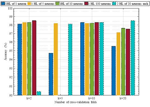
Fig. 3. Accuracy of the neural network versus the number of hidden neurons for different number of cross-validation folds.

Fig. 4 shows the probability of detection as a function of the probability of false alarm for a neural network with a learning rate of 0.001 and a number of iterations equal to 400. The cross-Validation is considered in these experiments to compute the probability of detection. A total number of 20 folds is considered to calculate the probability of detection as a function of the probability of false alarm. From this figure, it can be seen that the proposed model has an area under the curve on average equal to 99%. The ROC curve of the structure with two hidden layers of 20 neurons each is above the curves corresponding to one hidden layers with 29 neurons and 100 neurons.

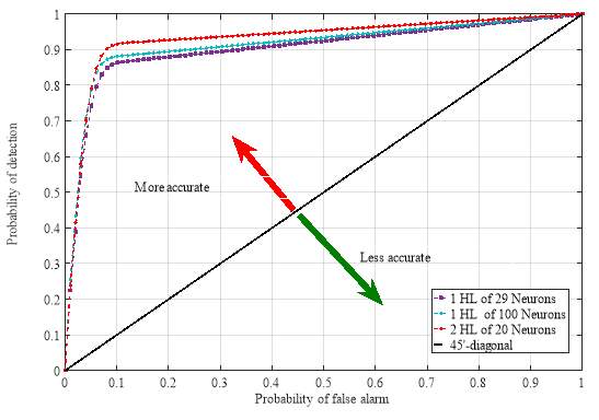
Fig. 4.  Probability of detection function of the probability of false alarm of the neural network.

Fig. 5 shows the accuracy of a neural network with two hidden layers of 20 hidden neurons each as a function of the number of iterations. The activation function is a relu function for the input layer, a hyperbolic tangent function for the hidden layer, and a sigmoid function for the output layer. For a number of iterations less than 200, one can see that for both training and testing, the accuracy increases as the number of iteration increases. However, for a number of iterations higher than 200, the accuracy for both the training and testing remains constant and is independent of the number of iterations. Fig. 6 shows the cross-entropy cost function versus the number of iterations for the same structure of the neural network.

From this figure, it can be observed that, for both training and testing, the cross-entropy cost function decreases as the number of iterations increases to reach a value less than 2% of error after 200 iterations. The results shown in this figure confirm those ones shown in Fig. 4. Indeed, when the cross-entropy cost function is minimized, it means that the accuracy of Table IV presents a comparison between the proposed model and the support vector machine with different kernels and with logistic regression. The comparison is performed considering four different evaluation metrics, the probability of detection, the probability of miss-detection, the probability of false alarm, and the accuracy.

From this table, one can see that SVM with a linear, RBF SVM, and logistic regression can achieve a high probability of detection of 100% while the proposed model achieves a probability of detection of 90.2%, which is less than SVM with logistic regression but higher than polynomial SVM with degree 3 which has a probability of detection of 84.27%. In terms of probability of miss-detection, Linear SVM, RBF SVM, and logistic regression have a probability of miss-detection of 0% while the proposed model has a probability of miss-detection of 9.8% and polynomial SVM has a probability of miss-detection of 15.7%. However, in terms of probability of false alarm, the proposed model has the lowest probability of detection, which is about 8%, followed by linear SVM with 39%, logistic regression with 39.24%, RBF SVM with 49.33%, and then polynomial SVM with 49.51%. In terms of the accuracy, the proposed model has the highest accuracy with 98.5%, followed by linear SVM with 81.2%, logistic regression with 80.68%, RBF SVM with 78.68%, and finally polynomial SVM with 69.12%.

As a conclusion, it can be said that the proposed model has the highest accuracy even if it has the lowest probability of detection compared to linear SVM, RBF SVM, and logistic regression because these algorithms show a very high probability of false alarm, which reduces their accuracy.

TABLE IV. Performance Comparison of The Proposed Model With SVM

Classifier	Probability of detection	Probability of miss-detection	Probability of false alarm	Accuracy
NN	90.2%	9.8%	8%	98.5%
Linear SVM	100.0%	0%	39%	81.2%
Polynomial SVM, degree 3	84.27%	15.7%	46.51%	69.12%
RBF SVM	100.0%	0%	43.33%	78.68%
Logistic regression	100%	0%	39.24%	80.68%

IV. Conclusion

Cognitive radio technology is a smart wireless solution that addresses the scarcity and underutilization of the radio spectrum. In cognitive radio networks, spectrum sensing plays a key role to allow secondary users to access free frequency channels. In the cooperative spectrum sensing, a secondary user relies on other users to determine the availability of frequency channel, which makes cognitive radio networks vulnerable to spectrum sensing data falsification attacks. Malicious users can take advantage of the cooperative nature of the sensing process to stop users from using the free licensed channels or use them for their own communications.

In this paper, we proposed a neural network-based approach to detect malicious users involved in the cooperative spectrum sensing process. A dataset is generated to train the proposed model, in which the energy statistic, the signal-to-noise ratio at the level of each secondary user, and the distance between the primary user signal and the secondary users are used for the classification. A series of experiments are conducted to test the validity of the proposed model using several metrics such as the probabilities of detection, miss-detection, and false alarm. The experimental results show that the proposed technique has a probability of detection as high as 90.2% and a probability of false alarm as less as 8%.

The proposed model is compared with other machine learning based techniques, such as support vector machine with different kernels and logistic regression. The proposed model outperforms the other techniques regarding the accuracy even if the probability of detection of linear SVM, RBF SVM, and logistic regression have higher probabilities of detection and lower probabilities of miss-detection; but, they have higher probabilities of false alarm compared to the proposed model. As a future work, deep neural network models for detecting spectrum sensing data falsification attacks in cooperative spectrum will be considered as these models does not have to deal with the feature selection.

References

[1] A. Al-fuqaha, S. Member, M. Guizani, M. Mohammadi, S. Member, Internet of Thing A Survey on Enabling tec pro app, 17 (2015) 2347–2376. doi:10.1109/COMST.2015.2444095.

[2] N. Kaabouch, W.C. Hu, Handbook of research on software-defined and cognitive radio technologies for dynamic spectrum management, IGI Global, 2014.

[3] N. Panwar, S. Sharma, A.K. Singh, A survey on 5G: The next generation of mobile communication, Phys. Commun. 18 (2016) 64–84. doi:10.1016/J.PHYCOM.2015.10.006.

[4] Cognitive Radio Technology, Elsevier, 2006. doi:10.1016/B978-0-7506-7952-7.X5000-4.

[5] I.F. Akyildiz, W.-Y. Lee, M.C. Vuran, S. Mohanty, NeXt generation/dynamic spectrum access/cognitive radio wireless networks: A survey, Comput. Networks. 50 (2006) 2127–2159. doi:10.1016/J.COMNET.2006.05.001.

[6] T. Yucek, H. Arslan, A survey of spectrum sensing algorithms for cognitive radio applications, IEEE Commun. Surv. Tutorials. 11 (2009) 116–130. doi:10.1109/SURV.2009.090109.

[7] J. Wu, T. Luo, G. Yue, An Energy Detection Algorithm Based on Double-Threshold in Cognitive Radio Systems, in: 2009 First Int. Conf. Inf. Sci. Eng., IEEE, 2009: pp. 493–496. doi:10.1109/ICISE.2009.257.

[8] S. Xie, L. Shen, J. Liu, Optimal threshold of energy detection for spectrum sensing in cognitive radio, in: 2009 Int. Conf. Wirel. Commun. Signal Process., IEEE, 2009: pp. 1–5. doi:10.1109/WCSP.2009.5371719.

[9] K. Srisomboon, A. Prayote, W. Lee, Double constraints adaptive energy detection for spectrum sensing in cognitive radio networks, in: 2015 Eighth Int. Conf. Mob. Comput. Ubiquitous Netw., IEEE, 2015: pp. 76–77. doi:10.1109/ICMU.2015.7061037.

[10] P. Semba Yawada, A.J. Wei, Cyclostationary Detection Based on Non-cooperative spectrum sensing in cognitive radio network, in: 2016 IEEE Int. Conf. Cyber Technol. Autom. Control. Intell. Syst., IEEE, 2016: pp. 184–187. doi:10.1109/CYBER.2016.7574819.

[11] H. Reyes, S. Subramaniam, N. Kaabouch, W.C. Hu, A spectrum sensing technique based on autocorrelation and Euclidean distance and its comparison with energy detection for cognitive radio networks, Comput. Electr. Eng. 52 (2016) 319–327. doi:10.1016/j.compeleceng.2015.05.015.

[12] M. Yang, Y. Li, X. Liu, W. Tang, Cyclostationary feature detection based spectrum sensing algorithm under complicated electromagnetic environment in cognitive radio networks, China Commun. 12 (2015) 35–44. doi:10.1109/CC.2015.7275257.

[13] F. Salahdine, H. El Ghazi, N. Kaabouch, W.F. Fihri, Matched filter detection with dynamic threshold for cognitive radio networks, in: 2015 Int. Conf. Wirel. Networks Mob. Commun., IEEE, 2015: pp. 1–6. doi:10.1109/WINCOM.2015.7381345.

[14] X. Zhang, R. Chai, F. Gao, Matched filter based spectrum sensing and power level detection for cognitive radio network, in: 2014 IEEE Glob. Conf. Signal Inf. Process., IEEE, 2014: pp. 1267–1270. doi:10.1109/GlobalSIP.2014.7032326.

[15] Q. Lv, F. Gao, Matched filter based spectrum sensing and power level recognition with multiple antennas, in: 2015 IEEE China Summit Int. Conf. Signal Inf. Process., IEEE, 2015: pp. 305–309. doi:10.1109/ChinaSIP.2015.7230413.

[16] I.F. Akyildiz, B.F. Lo, R. Balakrishnan, Cooperative spectrum sensing in cognitive radio networks: A survey, Phys. Commun. 4 (2011) 40–62. doi:10.1016/J.PHYCOM.2010.12.003.

[17] A. Ghasemi, E.S. Sousa, Collaborative spectrum sensing for opportunistic access in fading environments, in: First IEEE Int. Symp. New Front. Dyn. Spectr. Access Networks, 2005. DySPAN 2005., IEEE, n.d.: pp. 131–136. doi:10.1109/DYSPAN.2005.1542627.

[18] E. Visotsky, S. Kuffner, R. Peterson, On collaborative detection of TV transmissions in support of dynamic spectrum sharing, in: First IEEE Int. Symp. New Front. Dyn. Spectr. Access Networks, 2005. DySPAN 2005., IEEE, n.d.: pp. 338–345. doi:10.1109/DYSPAN.2005.1542650.

[19] C. Guo, T. Peng, S. Xu, H. Wang, W. Wang, Cooperative Spectrum Sensing with Cluster-Based Architecture in Cognitive Radio Networks, in: VTC Spring 2009 - IEEE 69th Veh. Technol. Conf., IEEE, 2009: pp. 1–5. doi:10.1109/VETECS.2009.5073471.

[20] W. Zhang, R. Mallik, K. Letaief, Optimization of cooperative spectrum sensing with energy detection in cognitive radio networks, IEEE Trans. Wirel. Commun. 8 (2009) 5761–5766. doi:10.1109/TWC.2009.12.081710.

[21] Jun Ma, Guodong Zhao, Ye Li, Soft Combination and Detection for Cooperative Spectrum Sensing in Cognitive Radio Networks, IEEE Trans. Wirel. Commun. 7 (2008) 4502–4507. doi:10.1109/T-WC.2008.070941.

[22] A. Ali, W. Hamouda, Advances on Spectrum Sensing for Cognitive Radio Networks: Theory and Applications, IEEE Commun. Surv. Tutorials. (2016) 1–1. doi:10.1109/COMST.2016.2631080.

[23] D.M.M. Plata, Á.G.A. Reátiga, Evaluation of energy detection for spectrum sensing based on the dynamic selection of detection-threshold, Procedia Eng. 35 (2012) 135–143. doi:10.1016/j.proeng.2012.04.174.

[24] M.R. Manesh, M.S. Apu, N. Kaabouch, W.-C. Hu, Performance evaluation of spectrum sensing techniques for cognitive radio systems, in: 2016 IEEE 7th Annu. Ubiquitous Comput. Electron. Mob. Commun. Conf., IEEE, 2016: pp. 1–7. doi:10.1109/UEMCON.2016.7777829.

[25] S. Mapunya, M. Velempini, Investigating Spectrum Sensing Security Threats in Cognitive Radio Networks, in: Springer, Cham, 2018: pp. 60–68. doi:10.1007/978-3-319-74439-1_6.

[26] A. Attar, H. Tang, A. V. Vasilakos, F.R. Yu, V.C.M. Leung, A Survey of Security Challenges in Cognitive Radio Networks: Solutions and Future Research Directions, Proc. IEEE. 100 (2012) 3172–3186. doi:10.1109/JPROC.2012.2208211.

[27] W. Fassi Fihri, H. El Ghazi, N. Kaabouch, B.A. El Majd, A Particle Swarm Optimization Based algorithm for Primary User Emulation attack detection, in: Submitt. to Int. Conf. Cybersecurity Conf., 2017.

[28] Z. El Mrabet, Y. Arjoune, H. El Ghazi, B.A. Al Majd, N. Kaabouch, Z. El Mrabet, Y. Arjoune, H. El Ghazi, B. Abou Al Majd, N. Kaabouch, Primary User Emulation Attacks: A Detection Technique Based on Kalman Filter, J. Sens. Actuator Networks. 7 (2018) 26. doi:10.3390/jsan7030026.

[29] F. Slimeni, B. Scheers, Z. Chtourou, V. Le Nir, R. Attia, Cognitive Radio Jamming Mitigation using Markov Decision Process and Reinforcement Learning, Procedia Comput. Sci. 73 (2015) 199–208. doi:10.1016/J.PROCS.2015.12.013.

[30] R. Di Pietro, G. Oligeri, Jamming mitigation in cognitive radio networks, IEEE Netw. 27 (2013) 10–15. doi:10.1109/MNET.2013.6523802.

[31] L. Zhang, G. Ding, Q. Wu, Y. Zou, Z. Han, J. Wang, Byzantine Attack and Defense in Cognitive Radio Networks: A Survey, IEEE Commun. Surv. Tutorials. 17 (2015) 1342–1363. doi:10.1109/COMST.2015.2422735.

[32] G. Mantas, N. Komninos, J. Rodriguez, E. Logota, H. Marques, Security for 5G Communications, in: Fundam. 5G Mob. Networks, John Wiley & Sons, Ltd, Chichester, UK, 2015: pp. 207–220. doi:10.1002/9781118867464.ch9.

[33] M. Khasawneh, A. Agarwal, A Collaborative Approach towards Securing Spectrum Sensing in Cognitive Radio Networks, Procedia Comput. Sci. 94 (2016) 302–309. doi:10.1016/J.PROCS.2016.08.045.

[34] R. Bouraoui, H. Besbes, Cooperative spectrum sensing for cognitive radio networks: Fusion rules performance analysis, in: 2016 Int. Wirel. Commun. Mob. Comput. Conf., IEEE, 2016: pp. 493–498. doi:10.1109/IWCMC.2016.7577107.

[35] M. Khasawneh, A. Agarwal, A Collaborative Approach for Monitoring Nodes Behavior during Spectrum Sensing to Mitigate Multiple Attacks in Cognitive Radio Networks, Secur. Commun. Networks. 2017 (2017) 1–16. doi:10.1155/2017/3261058.

[36] R. Chen, J.-M. Park, K. Bian, Robust Distributed Spectrum Sensing in Cognitive Radio Networks, in: IEEE INFOCOM 2008 - 27th Conf. Comput. Commun., IEEE, 2008: pp. 1876–1884. doi:10.1109/INFOCOM.2008.251.

[37] A.S. Rawat, P. Anand, H. Chen, P.K. Varshney, Collaborative Spectrum Sensing in the Presence of Byzantine Attacks in Cognitive Radio Networks, IEEE Trans. Signal Process. 59 (2011) 774–786. doi:10.1109/TSP.2010.2091277.

[38] N. NGUYEN-THANH, I. KOO, A Robust Secure Cooperative Spectrum Sensing Scheme Based on Evidence Theory and Robust Statistics in Cognitive Radio, IEICE Trans. Commun. E92–B (2009) 3644–3652. doi:10.1587/transcom.E92.B.3644.

[39] F. Adelantado, C. Verikoukis, A Non-Parametric Statistical Approach for Malicious Users Detection in Cognitive Wireless Ad-Hoc Networks, in: 2011 IEEE Int. Conf. Commun., IEEE, 2011: pp. 1–5. doi:10.1109/icc.2011.5963004.

[40] B. Kasiri, J. Cai, A.S. Alfa, Secure cooperative multi-channel spectrum sensing in cognitive radio networks, in: 2011 - MILCOM 2011 Mil. Commun. Conf., IEEE, 2011: pp. 272–276. doi:10.1109/MILCOM.2011.6127674.

[41] F. Adelantado, C. Verikoukis, Detection of malicious users in cognitive radio ad hoc networks: A non-parametric statistical approach, Ad Hoc Networks. 11 (2013) 2367–2380. doi:10.1016/J.ADHOC.2013.06.002.

[42] Y.E. Sagduyu, Securing Cognitive Radio Networks with Dynamic Trust against Spectrum Sensing Data Falsification, in: 2014 IEEE Mil. Commun. Conf., IEEE, 2014: pp. 235–241. doi:10.1109/MILCOM.2014.44.

[43] F. Zhu, S.-W. Seo, Enhanced robust cooperative spectrum sensing in cognitive radio, J. Commun. Networks. 11 (2009) 122–133. doi:10.1109/JCN.2009.6391387.

[44] Minho Jo, Longzhe Han, Dohoon Kim, H.P. In, Selfish attacks and detection in cognitive radio Ad-Hoc networks, IEEE Netw. 27 (2013) 46–50. doi:10.1109/MNET.2013.6523808.

[45] K. Arshad, K. Moessner, Robust collaborative spectrum sensing in the presence of deleterious users, IET Commun. 7 (2013) 49–56. doi:10.1049/iet-com.2012.0082.

[46] F.R. Yu, H. Tang, M. Huang, Z. Li, P.C. Mason, Defense against spectrum sensing data falsification attacks in mobile ad hoc networks with cognitive radios, in: MILCOM 2009 - 2009 IEEE Mil. Commun. Conf., IEEE, 2009: pp. 1–7. doi:10.1109/MILCOM.2009.5379832.

[47] P. Kaligineedi, M. Khabbazian, V.K. Bhargava, Secure Cooperative Sensing Techniques for Cognitive Radio Systems, in: 2008 IEEE Int. Conf. Commun., IEEE, 2008: pp. 3406–3410. doi:10.1109/ICC.2008.640.

[48] T. Zhao, Y. Zhao, A New Cooperative Detection Technique with Malicious User Suppression, in: 2009 IEEE Int. Conf. Commun., IEEE, 2009: pp. 1–5. doi:10.1109/ICC.2009.5198638.

[49] P. Kaligineedi, M. Khabbazian, V.K. Bhargava, Malicious User Detection in a Cognitive Radio Cooperative Sensing System, IEEE Trans. Wirel. Commun. 9 (2010) 2488–2497. doi:10.1109/TWC.2010.061510.090395.

[50] H. Li, X. Cheng, K. Li, C. Hu, N. Zhang, W. Xue, Robust Collaborative Spectrum Sensing Schemes for Cognitive Radio Networks, IEEE Trans. Parallel Distrib. Syst. 25 (2014) 2190–2200. doi:10.1109/TPDS.2013.73.

[51] T. Zhang, R. Safavi-Naini, Z. Li, ReDiSen: Reputation-based secure cooperative sensing in distributed cognitive radio networks, in: 2013 IEEE Int. Conf. Commun., IEEE, 2013: pp. 2601–2605. doi:10.1109/ICC.2013.6654927.

[52] H. Li, Z. Han, Catch Me if You Can: An Abnormality Detection Approach for Collaborative Spectrum Sensing in Cognitive Radio Networks, IEEE Trans. Wirel. Commun. 9 (2010) 3554–3565. doi:10.1109/TWC.2010.091510.100315.

[53] A. Vempaty, K. Agrawal, P. Varshney, H. Chen, Adaptive learning of Byzantines’ behavior in cooperative spectrum sensing, in: 2011 IEEE Wirel. Commun. Netw. Conf., IEEE, 2011: pp. 1310–1315. doi:10.1109/WCNC.2011.5779320.

[54] S. Li, H. Zhu, B. Yang, C. Chen, X. Guan, Believe Yourself: A User-Centric Misbehavior Detection Scheme for Secure Collaborative Spectrum Sensing, in: 2011 IEEE Int. Conf. Commun., IEEE, 2011: pp. 1–5. doi:10.1109/icc.2011.5962946.

[55] Xiaofan He, Huaiyu Dai, Peng Ning, HMM-Based Malicious User Detection for Robust Collaborative Spectrum Sensing, IEEE J. Sel. Areas Commun. 31 (2013) 2196–2208. doi:10.1109/JSAC.2013.131119.

[56] Jinlong Wang, Junnan Yao, Qihui Wu, Stealthy-Attacker Detection With a Multidimensional Feature Vector for Collaborative Spectrum Sensing, IEEE Trans. Veh. Technol. 62 (2013) 3996–4009. doi:10.1109/TVT.2013.2262008.

[57] Mingchen Wang, Bin Liu, Chi Zhang, Detection of collaborative SSDF attacks using abnormality detection algorithm in cognitive radio networks, in: 2013 IEEE Int. Conf. Commun. Work., IEEE, 2013: pp. 342–346. doi:10.1109/ICCW.2013.6649256.

[58] S.S. Kalamkar, P.K. Singh, A. Banerjee, Block Outlier Methods for Malicious User Detection in Cooperative Spectrum Sensing, in: 2014 IEEE 79th Veh. Technol. Conf. (VTC Spring), IEEE, 2014: pp. 1–5. doi:10.1109/VTCSpring.2014.7022848.

[59] X. He, H. Dai, P. Ning, A Byzantine Attack Defender in Cognitive Radio Networks: The Conditional Frequency Check, IEEE Trans. Wirel. Commun. 12 (2013) 2512–2523. doi:10.1109/TWC.2013.031313.121551.

[60] Y. Han, Q. Chen, J.-X. Wang, An Enhanced D-S Theory Cooperative Spectrum Sensing Algorithm against SSDF Attack, in: 2012 IEEE 75th Veh. Technol. Conf. (VTC Spring), IEEE, 2012: pp. 1–5. doi:10.1109/VETECS.2012.6240040.

[61] L. Duan, A.W. Min, J. Huang, K.G. Shin, Attack Prevention for Collaborative Spectrum Sensing in Cognitive Radio Networks, IEEE J. Sel. Areas Commun. 30 (2012) 1658–1665. doi:10.1109/JSAC.2012.121009.

[62] S. Sodagari, A. Attar, V.C.M. Leung, S.G. Bilen, Denial of Service Attacks in Cognitive Radio Networks through Channel Eviction Triggering, in: 2010 IEEE Glob. Telecommun. Conf. GLOBECOM 2010, IEEE, 2010: pp. 1–5. doi:10.1109/GLOCOM.2010.5683177.

[63] W. Wang, L. Chen, K.G. Shin, L. Duan, Secure cooperative spectrum sensing and access against intelligent malicious behaviors, in: IEEE INFOCOM 2014 - IEEE Conf. Comput. Commun., IEEE, 2014: pp. 1267–1275. doi:10.1109/INFOCOM.2014.6848059.

[64] G. Ding, Q. Wu, Y.-D. Yao, J. Wang, Y. Chen, Kernel-Based Learning for Statistical Signal Processing in Cognitive Radio Networks: Theoretical Foundations, Example Applications, and Future Directions, IEEE Signal Process. Mag. 30 (2013) 126–136. doi:10.1109/MSP.2013.2251071.

[65] Yang Li, Q. Peng, Achieving secure spectrum sensing in presence of malicious attacks utilizing unsupervised machine learning, in: MILCOM 2016 - 2016 IEEE Mil. Commun. Conf., IEEE, 2016: pp. 174–179. doi:10.1109/MILCOM.2016.7795321.

[66] G. Nie, G. Ding, L. Zhang, Q. Wu, Byzantine Defense in Collaborative Spectrum Sensing via Bayesian Learning, IEEE Access. 5 (2017) 20089–20098. doi:10.1109/ACCESS.2017.2756992.

[67] F. Farmani, M. Abbasi-Jannatabad, R. Berangi, Detection of SSDF Attack Using SVDD Algorithm in Cognitive Radio Networks, in: 2011 Third Int. Conf. Comput. Intell. Commun. Syst. Networks, IEEE, 2011: pp. 201–204. doi:10.1109/CICSyN.2011.51.

[68] Z. Cheng, T. Song, J. Zhang, J. Hu, Y. Hu, L. Shen, X. Li, J. Wu, Self-organizing map-based scheme against probabilistic SSDF attack in cognitive radio networks, in: 2017 9th Int. Conf. Wirel. Commun. Signal Process., IEEE, 2017: pp. 1–6. doi:10.1109/WCSP.2017.8170994.

[69] S. Shalev-Shwartz, S. Ben-David, Understanding Machine Learning, Cambridge University Press, Cambridge, 2014. doi:10.1017/CBO9781107298019.

[70] M. Hamid, N. Bjorsell, S. Ben Slimane, Sample covariance matrix eigenvalues based blind SNR estimation, in: 2014 IEEE Int. Instrum. Meas. Technol. Conf. Proc., IEEE, 2014: pp. 718–722. doi:10.1109/I2MTC.2014.6860836.

[71] M.R. Manesh, A. Quadri, S. Subramaniam, N. Kaabouch, An optimized SNR estimation technique using particle swarm optimization algorithm, in: 2017 IEEE 7th Annu. Comput. Commun. Work. Conf., IEEE, 2017: pp. 1–6. doi:10.1109/CCWC.2017.7868387.