ABSTRACT

The age of autonomous vehicles and systems are upon us sooner than we thought. The capability to autonomously navigate in an environment requires a lot of different sensors to work together and make sense of the data that they produce. The most important requirement of an autonomous system is the capability to map and localise itself in a given environment. Simultaneous Localisation and Mapping (SLAM) is the process by which an autonomous system makes sense of its environment.

The applications of autonomous systems are of wide variety ranging from military to warehouse or household. The autonomous vehicle is a combination of several key components like, cameras, image-processing capabilities, microprocessors and mapping technology etc.

In our project, we aim to focus on the mapping and localisation issue, or more commonly called as the SLAM issue. SLAM is basically probabilistic, meaning that it basically estimates the likelihood of something being there in the environment, by taking sensor data and establishing the chances of an obstacle being in its way.  Localisation can be done using several techniques like histogram filter, Kalman filter, Particle filter etc. In our project, the focus is on the implementation of different SLAM techniques and compare how they react in different situations. We use a Kinect sensor and data from the IMU for mapping and localisation while testing the computational power of the nVIDIA Jetson TX1. nVIDIA have successfully been able to attract interest from the automotive industry with their processors. Their processors are known to be superfast and are proven to have an exceptional ability to fuse images from cameras and radar sensors to detect obstacles.

Keywords:

Microsoft Kinect, autonomous, particle filter,

ABSTRACT

ACKNOWLEDGEMENTS

LIST OF FIGURES

LIST OF TABLES

LIST OF EQUATIONS

LIST OF ABBREVIATIONS

1 CHAPTER TITLE (USE HEADING 1)

1.1 Section Heading (use Heading 2)

1.1.1 Subsection Heading (use Heading 3)

1.2 Section Breaks

1.3 Inserting captions in the main document

1.3.1 Referring to captions for figures, tables etc

1.4 Updating Tables of Contents, Lists of Figures and Captions

1.5 Inserting Landscape Pages

2 CHAPTER TITLE (USE HEADING 1)

2.1 Section Heading (use Heading 2)

2.1.1 Subsection Heading (use Heading 3)

3 CHAPTER TITLE (USE HEADING 1)

3.1 Section Heading (use Heading 2)

3.1.1 Subsection Heading (use Heading 3)

4 CHAPTER TITLE (USE HEADING 1)

4.1 Section Heading (use Heading 2)

4.1.1 Subsection Heading (use Heading 3)

5 CHAPTER TITLE (USE HEADING 1)

5.1 Section Heading (use Heading 2)

5.1.1 Subsection Heading (use Heading 3)

6 CHAPTER TITLE (USE HEADING 1)

6.1 Section Heading (use Heading 2)

6.1.1 Subsection Heading (use Heading 3)

7 CHAPTER TITLE (USE HEADING 1)

7.1 Section Heading (use Heading 2)

7.1.1 Subsection Heading (use Heading 3)

8 CHAPTER TITLE (USE HEADING 1)

8.1 Section Heading (use Heading 2)

8.1.1 Subsection Heading (use Heading 3)

9 CHAPTER TITLE (USE HEADING 1)

9.1 Section Heading (use Heading 2)

9.1.1 Subsection Heading (use Heading 3)

REFERENCES

APPENDICES

Appendix A Appendix Title (Use Heading 7)

LIST OF FIGURES

Figure 1‑1 A figure caption

LIST OF TABLES

Table 1‑1 A table caption

LIST OF EQUATIONS

(1‑1)

LIST OF ABBREVIATIONS

IT	Information Technology

1   INTRODUCTION

1.1   Background

In recent years, we have seen a drastic increase in the use of autonomous robots and machines in several industries. They have been widely used for several purposes ranging from military applications to warehouse logistics to households. They have been proven to be very useful and increases efficiency and does not have the human error factor attached to it. Building rich 3D maps of environments is an important task for mobile autonomous robotics, with applications in navigation, manipulation, semantic mapping etc.

SLAM is an area that has been receiving a lot of attention and a lot of research has been going into it recently because of its use in a lot of industries. SLAM does have a lot of military applications as well. It is a very integral part of an autonomous UGV. SLAM gives the UGV an ability to localize itself in an unknown location and map the location as well. This can be done with sensors of different choices. The SLAM algorithms that we have taken into consideration are RGB-D SLAM and ORBSLAM2.

The basis of this study is to evaluate the difference between two Simultaneous Localisation and Mapping (SLAM) methodologies taking into consideration different parameters for comparison. The setup uses an IMU and Microsoft Kinect One to implement SLAM. The algorithms that have been used are open sourced algorithm’s. This study gives us a clearer idea into the understanding of the two different methodologies and how they fare under different scenarios. We implement a sensor fusion methodology to fuse the data that is obtained from the sensors. We make use of the Robot Operating System (ROS), and open source RGB-D SLAM and ORBSLAM bundles are utilized for comparison.

1.2   Problem Statement

Simultaneous Localisation and Mapping (SLAM) consists in the concurrent construction of a model of the environment and estimation of the state of a robot that is placed in the environment. The ability to navigate by avoiding obstacles and plan an apt path for the robot are integral parts of an autonomous robot.

The need to use a map of the environment is of huge importance. The map is a requirement to support other tasks like path planning or provide intuitive visualisation for a human operator. Also, the map allows limiting the error committed in estimating the state of the robot. In a scenario where we do not use a map, there would be an accumulation of dead-reckoning error. With the help of a map the robot can ‘reset’ its localization error by revisiting known areas. Thus, SLAM finds application in all scenarios in which a prior map is not available and needs to be built. SLAM provides an appealing alternative to user built maps, showing that robot operation is possible in the absence of an ad hoc localization infrastructure.

Loop closure is a technique that is central to the concept of SLAM. If we take away Loop closure SLAM reduces to odometry. In our study, we make a comparison between two different SLAM methodologies and implement them with different sensors and a processing unit. However, the movement of the sensors is controlled manually while the mapping process is automated. SLAM will be ideally performed using a Microsoft Kinect V2 sensor which is an

1.3   Thesis Structure

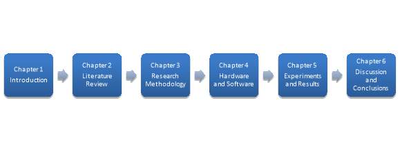
The structure of the this is illustrated in the Figure below. This thesis includes 5 other chapters other than the introduction. In chapter 2 we do a brief literature review on how to formulate the study and how this thesis can be useful for further research purposes. In Chapter 3 we discuss the Research methodology and explain the procedure followed for this research. In chapter 4 we review the Hardware and Software that we use along with its functioning. In chapter 5 we discuss the experiments and the results obtained. Finally, in chapter 6 we conclude by giving an explanation to the results and inferences. Additionally, future scope is also further mentioned.

Figure 1‑1 Thesis Structure

1.4   Summary

This chapter discusses the importance of the SLAM technology and how it is key for UGV’S and UAV technology. It highlights how the SLAM technology has evolved from the past and how the SLAM technology is proving to be useful in several other industries. We also mention the importance of using Robotic Operating System (ROS). The difference between the RGB-D RTAB mapping and ORBSLAM2 is touched upon.

2   LITERATURE REVIEW

2.1   Overview on SLAM

Simultaneous Localisation and Mapping is a process that is followed by robots usually to update its position on a map. The odometry of the Robot is generally erroneous, hence it cannot be reliable. Several other sensors can be used to correct the position of the robot. This is usually accomplished by mapping the environment and extracting features and re-observing. There will be landmarks that are identified on the map and it is based on these landmarks that the robot localises itself. The Kalman Filter keeps track of an estimate of the uncertainty in the robot’s position and the uncertainty in these landmarks it has seen in the environment. When the robot keeps moving the odometry keeps changing as well and the uncertainty pertaining to the robot’s new position is updated in the EKF using Odometry update. The landmarks are updated and are stored into a database. The robot attempts to associate the observed landmarks to the previously stored landmarks. If the observed landmarks cannot be associated with the landmarks that are stored in the data base then they are added as new observations. It is due to the inherent noise from the sensors, that SLAM is described by probabilistic tools.

There are several reasons as to why a map of the environment is very important for a robot/UGV/UAV. Two of the main reason why this is primary is stated:

• Required to support other tasks that are to be performed by the robot. For example, path planning, object recognition intuitive visualisation etc.
• Map allows limiting the error committed in estimating the state of the robot, i.e. dead reckoning could be quickly drifted in time. The map ensures that this does not happen.

SLAM finds an application in all situations or scenarios where there is no priori map and a map of the environment needs to be created. Of late, there have been recent developments in using SLAM for Virtual Reality and Augmented Reality applications.

The SLAM problem is extremely prevalent in the application of indoor robots. For example, indoor cleaning robots are required to create a map of the surroundings and constantly need to build and recognise landmarks so that it can localise itself. SLAM provides a better alternative to user built maps, this enables the robot to operate in the absence of an ad hoc localisation infrastructure.

The Classical age of SLAM is commonly referred to the period from 1986-2004. It is in this classical age that we saw the introduction of the main probabilistic formulations for SLAM, which include the EKF approach, the Rao-Blackwellised particle Filter, maximum likelihood estimation etc. It was in this period that the challenges like efficiency and robust data association was identified.

It is interesting to notice that the SLAM research that has been done over the past decade has produced the visual-inertial odometry algorithms. This is currently the state of the art SLAM method. Also, known as Visual Inertial Navigation (VIN), this method can be considered as a reduced SLAM approach wherein the loop closure module is disabled.

The SLAM methods ideally offer a natural defence against wrong data association and perceptual aliasing, which makes sure the robot is not deceived by similar looking environments. In this sense, we can say that the SLAM map provides us with a way to predict and validate our future measurements. This is key to ensure robust operation of the robot.

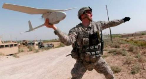
In several military applications SLAM has been proven to be useful. Many military UGV’S or UAV’S are entrusted with the task of exploring an environment and reporting a full 3D map to a human operator. Also several robots are capable of performing structural inspection. Figure shows several military grade UGV’s and UAV’s that use SLAM.

In the robotics community, “is SLAM solved?” is a well recurring question. This question is very difficult to answer because SLAM is very broad and can only be directed towards a given robot/environment/performance combination. There are several aspects when we implement SLAM:

• Robot: motion, sensors available, computational resource available.
• Environment: Planar or 3D space, natural and artificial landmarks present, risk of perceptual aliasing, amount of symmetry.
• Performance Requirements: Accuracy of state estimation of the robot, type of representation of the environment, success rate, estimation latency, max operation time, size of mapped area.

The sensors that are required for a robot are very much dependent on what is expected of the robot. At the same time the SLAM methodology that needs to be implemented on the robot is also dependent on the mission of the robot.

We are entering a new age or era of SLAM. The key requirements of a SLAM algorithm are changing. This new era can be referred to as the robust-perception age.  The key requirements can be characterised as mentioned below:

• Robust Performance: it is required to have a low failure rate throughout an extended period and through a broad set of environments. Must include fail safe and self-tuning capabilities.
• High Level Understanding: it is required to have a high level understanding of the environment rather than just the basic geometric perception of the environment. For example, semantics, physics, affordances);
• Resource Awareness: Resource awareness refers to the knowledge of the available sensing and computational resources. Adjusting the computational load depending on the available resources is expected.
• Task-driven Perception: System needs to be able to select the relevant perceptual information and filter out the irrelevant.

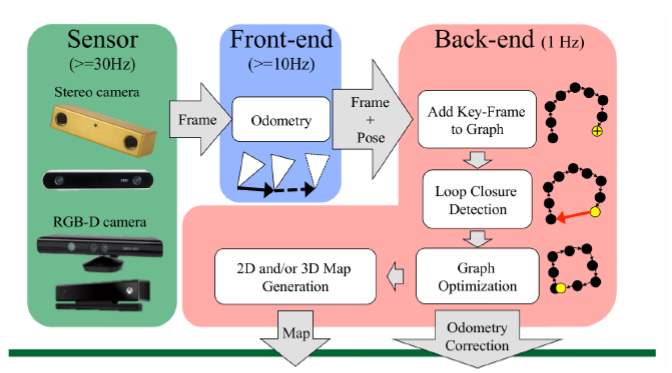
The figure shown below explains the two main components in the in the architecture of a SLAM system. The front end is responsible for abstracting sensor data that are flexible for estimation, and the back end is responsible for performing inference on the abstracted data produced by the front end.

2.2   Real Time Appearance Based Mapping (RTAB – MAP)

RTAB-Map can be better described as an RGB-D Graph based SLAM approach. This SLAM approach has two main key features, Loop closure detection and incremental appearance. The Loop closure detection that this approach uses is a bag-of-words method. This method is used in order to determine the likelihood of a new image coming from a previous location or if it is coming from a new location. Once this loop closure hypothesis is accepted, the map graphs add a new constraint. A graph optimiser is then used to minimise the errors in the map. The algorithm then uses a memory management approach to limit the number of locations that are used for the loop closure detection and for the graph optimisation. This is done so that real-time constraints on larger environments are respected. The advantage of RTAB map is that it can be used alone with a hand-held visual sensor or laser range finder. Fig 1 shows the system model and Fig 2 shows the quality of the 3D map generated using this algorithm. And Fig 3 compares the 2D map generated by a laser scan and the 2D generated map by RTAB. It can be noted that the map generated using RTAB is as good as a map generated using a laser sensor.

The loop closure feature will be explained in detail in the upcoming section. The Graph that the RTAB procedure generates consists of nodes and links. The nodes of the graph are responsible to save the odometry pose of each location of the map. Additional to this the map saves information like RGB images, depth images and visual words. Visual words will be explained under the loop closure section. The geometrical transformations between nodes are stored in the Links. The links are of two types: neighbour and loop closure. Links added between the current and previous nodes along with the odometery information are called Neighbour links and when a loop closure is detected between the current node and one from the same or previous maps, this is referred to as loop closure link.

2.2.1  Loop Closing:

Loop closing is the process of taking all the detected loop closures along with local estimated to minimise an error function. Typically, this error function describes the estimated trajectory of a sensor and minimising this error finds the most optimal trajectory given all the available measurements. Loop closing can be done both incrementally (optimise as loop closures are detected) or batch (optimise after all loop closures have been detected). Loop closing by optimising a graph based representation of the estimated sensor trajectory, which is commonly referred to as pose SLAM.

Given that the tracking of an RGBD camera over an extended sequence is successful, within some tolerance, over time the estimated pose of the RGBD camera will drift from its true pose. This drift can be corrected when the RGBD camera revisits an area of the environment which has already been mapped. This detection and recognition of previously mapped areas allows us to optimise the estimated trajectory of the RGBD sensor so that it is globally consistent. To a large extent, once the sensor poses have been determined a map of the environment can be created by overlaying the sensor data obtained at the poses.

2.2.2  Loop Closure Detection:

Loop closures can be defined as a point of a reconstructed environment in which there are multiple sensor readings, typically separated by a large temporal spacing. More simply, the sensor has returned to a previously visited area. Depending on the environment finding loop closures may or may not be necessary. For environments in which the sensor visits the same area multiple times the detection of loop closures is very prevalent, while very large environments where there is little or practically none, loop closing may not be prevalent. Correctly asserting these loop closures is important because any errors in the detection of loop closures will be manifested during loop closing, which could greatly affect the final reconstruction.

The global loop closure detection method uses a ‘bag of words’ approach and a visual dictionary is formed using feature extraction methods like SURF (Speeded up Robust Features) and SIFT (Scale Invariant Feature Transform).The loop closure hypothesis is evaluated using a Bayesian filter. A loop closure is detected when a loop closure hypothesis reaches a predefined threshold. Visual words are used to compute the likelihood required by the filter. The RGB image from which the visual words are to be extracted. is combined with a depth image, i.e., for each 2D point in the RGB image a corresponding 3D position can be computed using the calibration matrix and the depth information given by the depth image. When loop closure is detected, the rigid transformation between the matching images is computed by a RANSAC approach using the 3D visual word correspondences. If a minimum number of inliers are found, loop closure is accepted and a link with this transformation between the current node and the loop closure hypothesis node is added to the graph. RANSAC essentially provides a yes or no answer to determine whether loop closure has been completed.

2.3   ORB SLAM2

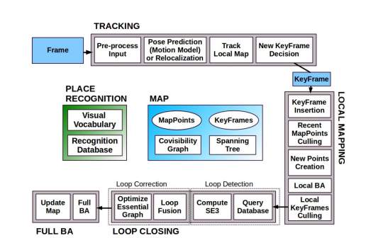
ORB SLAM is a visual SLAM algorithm that uses the ORB features to perform SLAM. The key feature to this algorithm is that it does not require external odometery data as compared to other SLAM algorithms. The fig below shows the system overview. The ORB SLAM algorithm is based on three main parallel thread as mentioned below:

1. Tracking: This thread is responsible for localising the camera with respect to every frame by finding feature matches to the local map. It also minimizes the reprojection error by applying motion-only BA (Bundle Adjustment).
2. Local Mapping: This thread performs local BA to manage the local map and to optimize it.
3. Loop Closing: In order to detect large loops and correct the accumulated drift by performing a pose graph optimization. This thread then launches a fourth thread to perform full BA after pose graph optimization.

The System architecture has a Place recognition module that is based on Bag-of words approach for re-localisation purposes. This proves to be useful in case of tracking failure or re-initialization of an already mapped scene or for loop detection. A co-visibility graph is maintained, this links any two key frames observing common points and a minimum spanning tree connecting all key frames.

The system makes use of ORB features for tracking mapping and place recognition purposes. The reason why ORB features are uses is because they have been proven to be robust to rotation and scale and they present a very good invariance to auto-gain and auto-exposure and illumination changes. They are proven to be fast to extract and match allowing for real time operation and they show very good precision.

Once the robot is in the exploration phase there is a place recognition database that is automatically created. It is in this database that the bag-of-words representation of the current image obtained from the environment is stored. This image is bound to the specific position in the map. This database helps us to recognise current place when the features of the currently observed ORB descriptors are compared to the ones in the database.

3   Research Methodology

3.1   Introduction

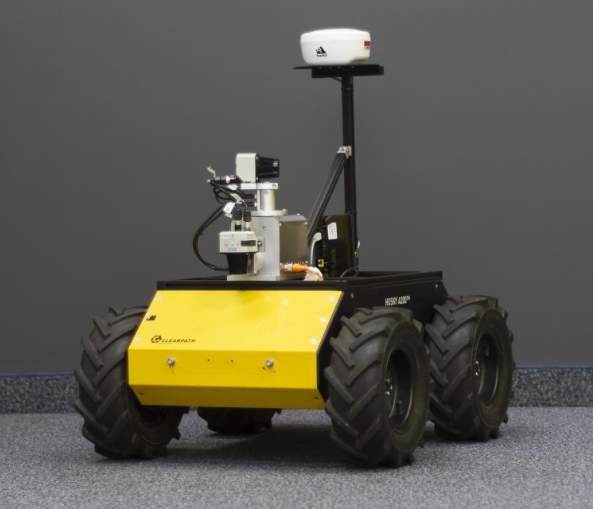
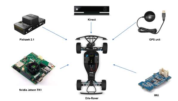
This research was initially intended to bring together several sensors together and build an autonomous UGV as shown in Fig. Due to delivery failure of certain components and considering the limitation of time the research intention had to be changed. It was then finalised that the intention of this research would be to implement two different SLAM methodologies and compare them. The outcome of the thesis was focused on understanding which SLAM methodology would be ideal to use on a UGV given the computational limitations, accuracy required, sampling rate etc. In this project we use two sensors, the Microsoft Kinect One and an IMU sensor to generate an accurate map of the surroundings and try to localise.

3.2   Adopted Research Methodology

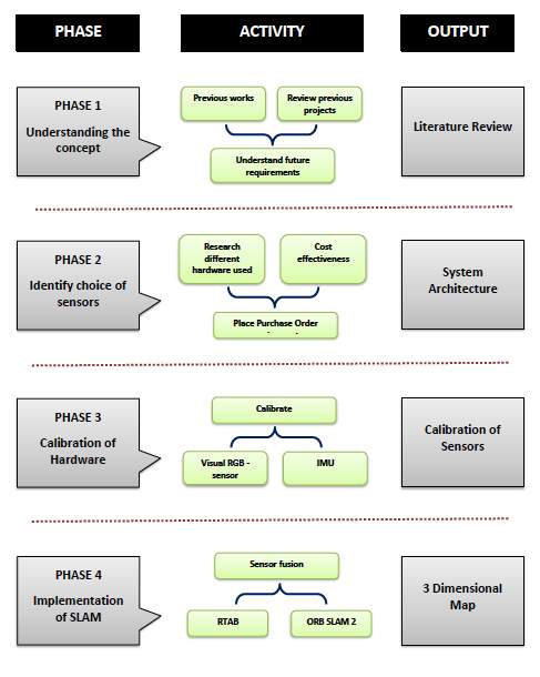
The diagram below shows the four phases adopted  for the research methodology which include Phase 1: Understanding concept of SLAM, Phase 2: Choice of sensors, Phase 3:  Calibration of Sensors, Phase 4: Sensor Fusion.

Phase 1: Understanding Concept of SLAM

This phase mainly involved gaining a better understanding of SLAM and the recent developments in its applications. An understanding of the past, present and future of SLAM was researched upon. A detailed literature review was conducted on the evolution of different SLAM techniques. It was then identified that RGB-D RTAB mapping and ORB-SLAM2 were the most commonly used SLAM techniques. The literature review was done from journals, books and thesis’s. The different applications of SLAM and the different industries that use SLAM were researched upon. After the review, it was evident that a comparative study between the two SLAM techniques have not been conducted. The comparative study would help in gaining a better understanding of which technique to adopt considering the scenario in which it is to be used.

Phase 2: Choice of Sensors

This phase mainly aims at understanding which sensors to use and why. A brief study was done based on previous projects and reports on the different sensors that have been used. Cost effectiveness was of primary importance while making a choice of sensors. A comparative study between different sensors and its accuracy was done. Data was collected based on previous studies and experiments. The output of this phase was to choose the sensors and create a system architecture of the sensors.

Phase 3: Calibration of Sensors

In this phase the hardware components were individually calibrated using several open source methods. The calibration of the vision sensor and the inertial measurement unit was done separately on the processing unit. The software that was used for the calibration method is an open source software called ROS (Robot Operating System) which is currently available only on Linux based processors.  A detailed procedural description is given in the Appendix. The error recorded before and after calibration is stated in the chapters below. It is necessary to perform the calibration of the sensors before any experiments are performed.

Phase 4 : Implementing SLAM

This phase focuses on implementing the selected two SLAM methodologies. The parameters of comparison are sampling rate, reaction to light, accuracy, computational load etc. The implementation of SLAM in the different methods gives us the different graphs and eventually creates a map of the environment. The Localisation of the system is also done, bear in mind the system is not mounted on a UGV in our experiments. The odometry and loop closure detections are done while implementing SLAM.

The table of comparison shows the results of the differences and it is possible to choose the SLAM method according to one’s own requirements.

The Implementation of SLAM also sees the sensor fusion that implemented for both the Kinect and IMU data.

4   Components and Architecture

4.1   Introduction

In the process of researching on the choice of hardware, a lot of different projects that involved the implementation of SLAM was taken into consideration. The processor and sensors were chosen keeping cost effectiveness in mind. It was initially finalised to make use of the Raspberry Pi 3 Model-B as the processing unit. Upon further research, it was understood that the Raspberry Pi-3 Model B did not have the sufficient computational power that is required by the choice of visual sensor which is the Microsoft Kinect One. The Microsoft Kinect One requires a USB 3.0 port for data transfer. Thus, leading to the choice of the Jetson TX1 as our processing unit.

The Microsoft Kinect One was the choice of sensor when compared to the Laser scanner. The accuracy of the Laser scanner was far superior when compared to the Microsoft Kinect, but the cost of the Microsoft Kinect One was very impressive.

The choice of IMU sensor was made based on the ease of connection to the Jetson TX1. The Adafruit IMU is a very cost effective sensor with I2C interface. The wiring and connections are further explained in the Experimental Procedure section.

4.2   Hardware

4.2.1  Microsoft Kinect One

The Microsoft Kinect One is a motion sensing device that is produced to be used with the Microsoft Xbox. There has been an evolution with the RGB-D cameras in the last decade. They are the first-choice sensors for several robotics and computer vision applications mainly due to its cost effectiveness. They are the preferred sensor when compared with laser scanners due to this reason. The laser scanners however have more accurate measurements. The Microsoft Kinect One has several industrial applications including real-time detections and detections on automotive systems. Recently they have been used for crime scene detection and forensic studies.

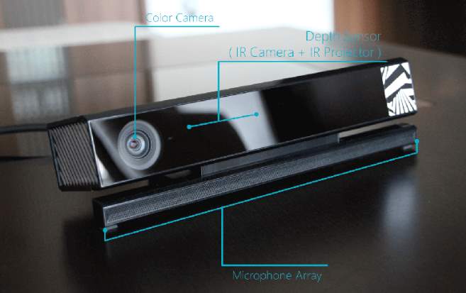
The Microsoft Kinect One comprises of two cameras, an RGB and an IR camera. The IR camera uses three IR blasters to enable active illumination of the environment. The specifications of the Kinect One are given in Table 1. The Kinect One unlike the Microsoft Kinect 360 uses a Time-of-flight method and has been an upgrade when compared to the Kinect 360 which uses a Pattern Projection principle. A comparison of the two devices has been shown in Table 2. This clearly shows that the Kinect One is an upgrade to the Kinect 360. In the Time of Flight (ToF) principle, the camera determines the depth by measuring the time the emitted light takes from the camera to the object and back. The Kinect One emits infrared light that has modulated waves and the phase shift of the returning light is then detected and thus gives us a depth image. The basic principle that the Kinect One uses is that if we know the speed of light we can say that the distance to be measured is proportional to the time that the active illumination target to travel from emitter to target. And this is how the Kinect V2 sensor acquires the distance to object measurement, for each pixel of the output data.

Technical features of Kinect One Sensor
Infrared Camera Resolution	512 x 424 pixels
RGB camera resolution	1920 x 1080 pixels
Field of View	70 x 60 degrees
Framerate	30 frames per second
Operative Measuring range	From 0.5m to 4.5m Between 1.4mm (@ 0.5m range)
Object pixel size (GSD)	12mm (@ 4.5m range)

The Microsoft Kinect is a vision based sensor that has several other sensors including an accelerometer, multi array microphones, 3-D depth sensors and an RGB sensor. The Kinect when compared to a laser scanner has an advantage in terms of the 3-D that it provides along with the cost effectiveness of it. The Kinect has a relatively fast sampling rate.

	Kinect V1	Kinect V2
Colour	640 x 480 @ 30fps	1920×1080 @ 30fps
Depth	640 x 480 @ 30fps	512 x 424 @ 30fps
Infrared	640 x 480 @ 30 fps	512 x 424 @ 30fps
Vertical Field of View	43 degrees	60 degrees
Horizontal Field of View	57 degrees	70 degrees
USB standard	2.0	3.0

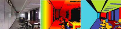
As shown in figure 2, we get three different outputs from the two camera’s of the Kinect One, namely the infrared image, depth map and the colour image. The depth image stores measurement information for each pixel and the point cloud is calculated using the distances that are measured using the depth map.

Either a mapping capacity gave by the SDK (Software Development Kit) is connected amongst profundity and camera space, or self-actualized arrangements can be utilized applying the point of view projection connections.This results in the point cloud image which is basically a list of (X, Y, Z) coordinates from the distance measurement. The colour frame has a higher resolution compared to the depth image and in order to extract colorimetric information, a transformation of the colour frame is to be performed. This transformation is obtained using the mapping function from the SDK. This enables us to map the corresponding colour to a corresponding pixel in depth space. Combined with the (X, Y, Z) coordinates from the depth map and the colour information we get the colorized point cloud.

It was noticed that there was an influence of temperature on the range measurements.  Different readings were observed at different temperatures. After referring to several papers on the Pre-heating time and Noise reduction of the Kinect One, we concluded that a pre-heating time of 30 minutes will be respected even if the distance variation is quite low.

Calibration Method: The Calibration method that we follow is using an open source driver from Thiemo Wiedemeyer, Institute of Artificial Intelligence, University of Bremen. This driver uses OpenCV to calibrate the two cameras, RGB and IR camera to each other. We use a chess board of dimensions 5 x 7 x 0.3m for calibration. The methodology used to calibrate is as follows:

• The calibration pattern is printed (5 x 7 x 0.3 m) and stuck onto a plain flat object. It is important to make sure that the calibration pattern is stuck onto the surface very flat without any irregularities. It is advisable to check the distance between the features of the printed pattern with the help of a caliper.  It is possible that the pattern can be scaled while printing. The distance between the black and white patterns need to be exactly 3cm apart.
• The Kinect One and the calibration pattern need to be mounted on a tripod. This is to make sure that the Kinect sensor is stable before an image is taken. The tripod helps us to keep track of the distance between the sensor and the pattern.
• When recording images for all the steps as shown below (RGB, IR, SYNC), start the recording program, and then spacebar is pressed to record. The calibration pattern should be detected and the image must appear to be clear and steady.
• It is ideal to record images of the calibration pattern in all areas of the image and at different orientations as well as different distances (at least two).
• We first start at a shorter distance where the calibration pattern covers most of the screen. Images are taken by tilting the pattern vertically and horizontally.
• Once the calibration at a short distance is done we move the calibration pattern further away. Then images of the calibration pattern are taken at different orientations such that the calibration pattern is present around most of the camera image. For example, first we calibration pattern is on the upper left corner and then on the next image it is on the upper middle and then on the upper right corner.

The calibration method is done using ROS which is installed on the nVIDIA Jetson TX1. ROS runs on the Ubuntu 14.04 flashed on the Jetson TX1.

4.2.2  nVIDIA Jetson TX1

The Jetson TX1 Developer kit is an nVIDIA based development platform that is ideally used for visual computing. The reason why the Jetson TX1 is an ideal platform for our experiments is because it has high computational performance and is of the perfect size to be mounted on a UGV. The TX1 has a USB 3.0 that is required for the Microsoft Kinect One’s data transfer. It comes with a Linux environment that is pre- flashed. It also comes with a camera module that we do not use. The board exposes a variety of standard hardware interfaces, which makes it a highly flexible and extensible platform. The module combines a 64-bit quad-core ARM cortex- A57 CPU with a 256-core Maxwell GPU. It comes equipped with 4 GB of LPDDR43200, 16 GB of eMMC Flash, 802.11ac Wi-Fi and Bluetooth.

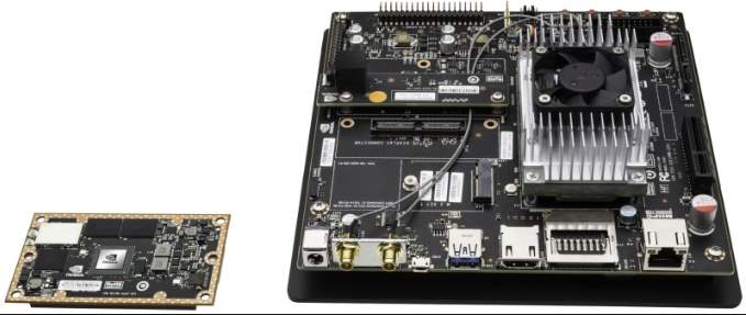
The Jetson TX1 can be seen as an upgrade to the Raspberry Pi model 3. It trounces the Raspberry pi in testing by a factor of about three. It can also be compared to the Intel NUC boards.

The problem with using the Jetson TX1 is that since it is such a recent platform, the community of users is only developing. The Jetson TX1 is specifically meant for engineers trying to build autonomous carts and for machine learning purposes.

Table 3 shows the specifications of the Jetson TX1 module. Though the Jetson TX1 is much more computationally superior to boards like the Raspberry Pi, the price between the two cannot be compared. The Jetson is much more expensive than the Raspberry Pi.

	JETSON TX1
GPU	1 TFLOP/ s 256-core Maxwell
CPU	64-bit ARM A57 CPUs
Memory	4 GB LPDDR4 | 25.6 GB/s
Storage	16 GB eMMC
Wi-Fi/ BT	802.11 2×2 ac/ BT Ready
Networking	1 Gigabit Ethernet
Size	50mm x 87mm
Interface	400 pin board-to-board connector

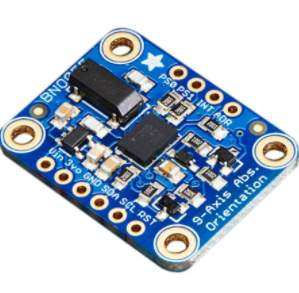
4.2.3  Adafruit BNO055 Absolute Orientation Sensor

The Bosch BNO055 is an impressive 9-DOF sensor. This sensor is straight forward to use and the advantage of this sensor is that it does not require to be calibrated as it comes pre calibrated. The sensor has a built in arm Cortex processor on it which is responsible for the integration of all the fusion data and outputs it in euler angles or quaternion angles. The sensor is directly connected on to the processing board and the pose estimate is found out. The BNO055 uses an I2C technique called ‘clock stretching’. The chip holds the SCL line low while taking a reading. This provides more flexibility on the I2C master side because it does not have to do a full command-and-response.

4.3   Software

4.3.1  ROS (Robot Operating System)

The experimental setup is based on the ROS environment which is a platform that provides an operating system like functionality on a computer. The advantage of using ROS is that it provides us with various standard operating system services like hardware abstraction, low-level device control, message passing between processes, and package management. It is based on graph architecture with a centralised topology where processing takes place in nodes that may receive or post, such as multiplex sensor, control, state, planning, actuator and so on. The availability of ROS is only on a few limited platforms like Ubuntu. We run our experiments on the Jetson TX1, which is our processing unit. The Ubuntu 14.04 was flashed on the Jetson TX1 and ROS was subsequently installed.

ROS is an algorithm diagram comprising of a set of nodes corresponding with each other over edges. ROS contains instruments for assessing the diagram and checking what is the topic said by node or by theme. Fig 2 shows the process of communication between nodes. One of the essential apparatuses of ROS, rostopic, permits a command line client to see what is constantly said regarding a subject, how oftentimes messages are, no doubt distributed, and so forth.

The ROS Computation Graph Level

The functioning of ROS comes down to nodes, the master, the Parameter Server, messages, services, topics and bags. These together provide data to the Computation Graph.

• Nodes are processes where computation is done. If you want to have a process that can interact with other nodes, you need to create a node with this process to connect it to the ROS network. Usually, a system will have many nodes to control different functions. You will see that it is better to have many nodes that provide only a single functionality, rather than a large node that makes everything in the system. Nodes are written with a ROS client library, for example, roscoe or sospy
• Master: The Master provides name registration and lookup for the rest of the nodes. If you don’t have it in your system, you can’t communicate with nodes, services messages and others. But it is possible to have it in a computer where nodes work in other computers.
• Parameter Server: The Parameter Server gives us the possibility to have data stored using keys in a central location. With this parameter, it is possible to configure nodes while its running or to change the working of the nodes.
• Messages: Nodes communicate with each other through messages. A message contains data that sends information to other nodes. ROS has many types of messages, and you can also develop your own type of message using standard messages.
• Topics: Each message must have a name to be routed by the ROS network. When a node is sending data, we say that the node is publishing a topic. Nodes can receive topics from other nodes simply by subscribing to the topic. A node can subscribe to a topic, and it isn’t necessary that the node is publishing this topic should exist. This permits us to decouple the production of the consumption. Its important that the name of the topic must be unique to avoid problems and confusion between topics with the same name.
• Services: When you publish topics, you are sending data in a many-to-many fashion but when you need a request or an answer from a node, you can’t do it with topics. The services give us the possibility to interact with nodes. Also, services must have a unique name. When a node has a service, all the nodes can communicate with it, thanks to ROS client libraries.
• Bags: Bags are a format to save and play back the ROS message data. Bags are an important mechanism for storing data, such as sensor data, that can be difficult to collect but is necessary for developing and testing algorithms. You will use bags a lot while working with complex robots.

Procedure:

In an ideal situation, the Kinect One would be mounted on top of a UGV and the robot will be driven into an unknown environment. The Kinect then takes a stereoscopic video of the environment. The video that is taken is then broken down into frames and is separated into RGB and Depth elements. We then use a feature extraction algorithm to locate landmarks and key points. The features that are extracted from the environment are then fused with the corresponding depth data and is then stored in a database. The feature extraction algorithm will be applied to every new frame and a data match is done after comparing the frame to the ones in the database. It will localise itself with respect to the landmarks.

REFERENCES

Insert list of references here

APPENDICES

Whilst Heading 1 to Heading 6 can be used to number headings in the main body of the thesis, Heading styles 7–9 have been modified specifically for lettered appendix headings with Heading 7 having the ‘Appendix’ prefix as shown below.

1. Appendix Title (Use Heading 7)
   1. Appendix Section (Use Heading 8)
      1. Appendix Subsection (Use Heading 9)
   2. Creating captions in Appendices

If you have chosen to include chapter numbers in your captions then follow the instructions given here to apply the same format to the captions in your appendices.  This section explains how to caption the figures and tables in your Appendices, assuming that Heading 7 is numbered “Appendix A” and that the Figures and Tables are going to be labelled ‘Figure A-1’, ‘Figure A-2’, ‘Table B-1’ etc.

You will have to create new, separate labels that look like the ‘Figure’ and ‘Table’ labels you used in the main body of your thesis.

1. Select the References tab on the Ribbon then click on Insert Caption
2. Click New Label.  Type Figure_Apx then click OK
3. You now have two labels for figures, called Figure and Figure_Apx
   Repeat for table captions.
4. In the Caption box, type your caption text
5. Click Numbering.  Tick Include chapter numbering and choose Heading 7 from the drop-down list of styles and click OK twice
6. Your caption should look something like this:

Figure_Apx A‑1 This is the caption text for a Figure in the Appendix

7. Delete the extraneous ‘_Apx’ from the caption label so it reads:
   Figure A‑1 This is the caption text for a Figure in the Appendix
   TIP: Instead of deleting each ‘_Apx’ individually use Find & Replace to modify all the labels at once.
   3. Creating Lists of Figures and Tables for Appendices

This template already includes a List of Figures and a List of Tables, however you will have to create two new lists for the ‘Figure_Apx’ and the ‘Table_Apx’ labels.

1. Place the insertion point on a blank row after the existing List of Figures
2. Select the Insert Table of Figures command on the References tab of the Ribbon
3. Set the Caption Label box to ‘Figure_Apx’ and click OK
   Note:  Word will put a single blank line between the original and new lists preventing it from appearing as one seamless list.  However if you select the blank paragraph between the tables you can hide it by opening the Font dialog box from the Home tab and selecting Hidden.
4. Click after the List of Tables and repeat for the Caption Label ‘Table_Apx’