A Probabilistic Model of Ballistic Missile Defense for Heterogeneous Targets

ABSTRACT

In this paper, we propose that during a complex engagement scenario with heterogeneous targets, the defence can use a SLS-OLEO (Shoot-Look-Shoot with Optimal Last Engagement Opportunity) firing tactic to optimize its (Probability of Raid Annihilation) at the last engagement opportunity.  To optimize this approach, we will compare various firing tactics using astrodynamics, calculus with constraints, perturbation theory, dynamical programming and generating functions, and the concavity characteristic of the .  In addition, we will consider how the contributes to the   (Probability of Integrated System Effectiveness), which in turn determines the global effectiveness of a BMDS (Ballistic Missile Defense System).

1 – INTRODUCTION

Current literature on BMDSs (Ballistic Missile Defense Systems) involves separate analyses that focus on isolated aspects of the overall system.  Specifically, there are studies on theoretical firing doctrines  (Soland 1987), Shoot-Look-Shoot tactics (Wilkening 1999), hit assessment (Weiner et al. 1994), orbital mechanics (Cranford 2000), and an integrated probabilistic model such as (Boeing Co 1999).  In contrast, this paper aims to focus on the (Probability of Raid Annihilation) as a core component of the (Probability of Integrated System Effectiveness), and therefore key to determining the effectiveness of the BMDS.

To demonstrate the importance of the , we will compare three firing tactics in an engagement scenario involving heterogeneous targets. After a critical comparison of the results, we will illustrate that while the SLS-OLEO (Shoot-Look-Shoot with Optimal Last Engagement Opportunity) does not yield the greatest , it presents the most practically effective in a complex engagement scenario. We will also explore where the   becomes a significant component of the BMDS framework, and suggest two tactics to boost the . Our hope is that members of the operations research community will be able to use these findings to evaluate the global effectiveness of a BMDS.

To help focus the problem, we define an example scenario of five heterogeneous re-entry vehicles (RVs) and an inventory of twenty interceptors, (Wilkening 1999).  This scenario is certainly not a saturated scenario where the number of RVs overwhelms the inventoty of interceptors as investigated by (Dou et al. 2010).  Due to the complexity of BMD (Ballistic Missile Defense), there are characteristics and approaches that we were unable to cover or analyze in depth in this paper.  In comparison to other studies, our perspective is one sided (defense only) as opposed to two sided (defense and offense, Brown et al. 2005).  We also examine mainly Ground Based Interceptors (GBIs), rather than other launching platforms such as a loitering aircraft (Burk et al. 2009), and do not consider decoys (Washburn 2005). We note that BMD could also be examined using agent based simulations (Garrett et al. 2011 and Holland et al. 2011), or modeled using Markov chains (Menq et al. 2007). The effects of framing human subjects in missile defense are examined by (Park and Rothrock 2006).  In spite of these assumptions and simplifications, we believe that our methodologies provide a simple way to understand BMD and offer a direct and unified approach to assess the effectiveness of a BMDS.

The paper is organized as follows:  Section 2 describes the number of engagement opportunities;  Section 3 presents three known firing tactics that can be used against identical (homogeneous) targets; Section 4 extends some of the firing tactics for heterogeneous targets and proposes a new tactic;  Section 5 describes the concavity of the ;  Section 6 uses concavity to determine the globally optimal ;  Section 7 illustrates the measures of effectiveness;  Section 8 discusses the and ways to improve it; and we conclude in Section 9.

This article is the full and expanded technical version of another essay paper published in 2014 (Nguyen 2014 which received the 2015 Koopman prize from the Institute for Operations Research and Management Sciences) with some new elements including the consideration of new firing tactics (in Section 4), the concavity of the (in Section 5) and the globally optimal (in Section 6). While the measures of effectiveness in Section 7 are accessible in existing literature, these measures of effectiveness are determined based on the novelty of Sections 4, 5 and 6.  To the best of our knowledge, there are no papers in the literature that tie all of these aspects together and present such a self-contained article on BMD.  Preliminary results of this article were published in a conference proceedings (Nguyen and Miah 2014) where we make use of the genetic algorithm to optimize the measures of effectiveness.  As well, the content was part of an internal document to Defence R&D Canada that is not available in the open literature.

2 – ENGAGEMENT OPPORTUNITIES

EOs (Engagement Opportunities) are chances for the defense to destroy an incoming warhead with a defensive weapon, and are essential to the evaluation of the .    Ultimately, for an EO to exist, there must be times when the trajectory of the interceptor can intersect the trajectory of the threat missile.  When and where these intersections occur is governed by the geometries of the trajectories, the early warning time the BMDS sensors provide, the speed of the command and control system (including the humans that may be in the loop) to control system components, and the performance capability of the interceptor.

To determine the number of engagement opportunities, we use two classic problems in astrodynamics: Kepler’s problem (Vallado 2001:pp. 88-103) and Lambert’s problem (Vallado 2001: pp. 445-447).  Kepler’s problem determines if a ballistic missile has enough energy to reach a given location, while Lambert’s problem determines if a ballistic missile can reach a given location in a given time.  Clearly, if a ballistic missile does not have sufficient energy to reach a given location, it will never reach that location in time.  Hence, we solve Kepler’s problem first to filter out cases without sufficient energy.  Kepler’s problem is also substantially less computationally intensive than Lambert’s problem, which reduces the amount of computation.

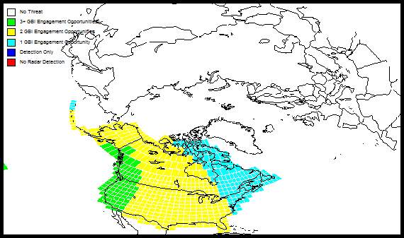
Figure 1 – Defended area footprint and engagement opportunities.

Kepler’s problem and Lambert’s problem are implemented in (Cranford 2000), which also includes sensor coverages, and command and control delays.  A typical output of (Cranford 2000) is shown in Figure 1, which displays the defended area footprint and the number of engagement opportunities.  For example, the cells on the West Coast of the USA indicate that the defense has three or more engagement opportunities against threats targeting these cells.

3 – EXISTING SHOOT-LOOK-SHOOT Firing doctrines

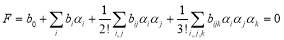
Firing doctrines are important to BMD – depending on the scenario, they can significantly improve or degrade the MOEs (Measures of Effectiveness) such as the and the(Expected Number of Interceptors Expended).  For instance, when the defense has only one engagement opportunity against each threat, it would be best to allocate the number of interceptors as evenly as possible among the threats – this is called the Salvo tactic.  When the defense has more than one engagement opportunity and perfect hit assessment after each engagement, then the defense can employ Soland’s tactic (Soland 1987) to optimize the . When the defense can engage each threat with a fixed-size salvo at each engagement opportunity, it can employ a Shoot-Look-Shoot tactic with Fixed Size Salvos (SLS-FSS), which also enhances the (Nguyen et al. 1997).  In this section, we shall consider these three firing doctrines: the Salvo Tactic, Soland’s tactic and the SLS-FSS tactic.

Before proceeding, we define the hit assessment as the capability to determine whether or not an RV has been hit by the interceptor(s).  There can be errors in hit assessment as described in (Yossi et al. 1997), however, in this paper we describe only the two extreme cases: one with no hit assessment (Salvo tactic) and the other with perfect hit assessment (ideal SLS tactics).  The associated firing MOEs and system MOE will be bounded by these two cases – no hit assessment and perfect hit assessment.

We can now describe the essence of each of these firing doctrines, using the following parameters:

1. is the number of threats.
2. is the number of engagement opportunities.
3. is the number of interceptors.
4. is the probability of a single hit.
5. is the probability of a single miss.
6. is the probability of a hit of a salvo of size .
7. is the probability of a miss of a salvo of size .

Note that for a non-trivial scenario, must be greater than or equal to one i.e. .

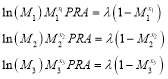
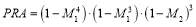
The Salvo tactic

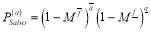
The Salvo tactic is the simplest tactic; The defence allocates interceptors as evenly as possible among the threats.  This allocation optimizes the when the defense has only one engagement opportunity.  The optimality was proved by (Soland 1987).  He showed that an uneven allocation provides a lower than that obtained from a more uniform allocation.  Hence, an allocation that is as uniform as possible yields the optimal .  (Soland 1987) also provides the following formulae for the MOEs.

The can be written as:

        (1)

while the expected number of interceptors is simply equal to the number of interceptors in the inventory:

          (2)

where

  

and

  

is the greatest integer less than or equal to while is the smallest integer greater than or equal to .  Note that the optimality of the above MOEs is true independently of the value of the single shot probability of hit ().

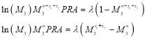
Soland’s tactic

If the defense’s architecture allows more than one engagement opportunity and perfect hit assessment after each engagement, then it can allocate interceptors using dynamical programming to optimize the (Soland 1987).  This is a natural generalization of the Salvo tactic – in fact, the Salvo tactic is a special case of Soland’s tactic where the defense has only one engagement opportunity.

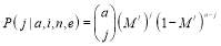
The optimality of Soland’s tactic is based on a recursion:

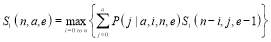      (3)

with boundary conditions

          (4)

         (5)

and

       (6)

where , interceptors are assigned to each RV.  is the probability that RVs survive the th engagement from the end when there are RVs left before that engagement and of remaining interceptors are used in an optimal manner at that engagement.  Note that in general, is not an integer.  When this is the case, of the RVs are assigned interceptors each and the remaining are assigned interceptors each.

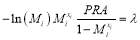
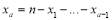
In addition, is the if engagement opportunities remain, the defense has interceptors left, there are RVs left undestroyed, and the defense follows an optimal policy for the remaining engagements.  The first boundary condition – – tells us that the is equal to if there are no threats.  The second boundary condition – 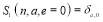where is the Kronecker Delta function – tells us that the is equal to zero if the defense has no engagement opportunity against the threats unless there are no threats.  That is, in which case the is equal to .

Essentially, the optimality of Soland’s tactic is based on two observations.  First, given a number of threats and a number of interceptors, the defense must allocate the number of interceptors as evenly as possible among the threats in order to optimize the at an engagement opportunity.  This is encoded in the probabilities.  Second, the defense must select the optimal number of interceptors allocated at each engagement opportunity against a given number of leakers, where a leaker is an RV that survives previous engagements.  This is done by computing numerically the for each possible allocation. In other words, for each where ranges from zero to , represents the number of interceptors allocated at the current engagement opportunity.  If the defense determines the that optimizes the , the remaining inventory interceptors will be allocated at subsequent engagement opportunities in an optimal way.

The Shoot-Look-Shoot with Fixed Size Salvo (SLS-FSS) tactic

The SLS-FSS tactic is a SLS (Shoot-Look-Shoot) tactic where the defense engages each threat with a Fixed Size Salvo (salvo of size say).  If a threat is missed then it is re-engaged with another fixed size salvo, provided the defense inventory and engagement opportunities allow doing so.  This SLS-FSS tactic minimizes the expected number of interceptors expended while maintaining the same (or yielding a better) than the one provided by the Salvo tactic if , (Nguyen et al. 1997).  However, this is not optimal in general, and contrastingly is typically lower than the one provided by Soland’s tactic.  Note that, the SLS-FSS tactic is sometimes mistakenly regarded as the optimal SLS tactic and hence the erroneous conclusion that the SLS tactic only saves the inventory of interceptors while providing the same as that of the Salvo tactic.  This misconception is incorrect for two reasons:  first, the SLS-FSS tactic provides a better than the one based on the Salvo tactic unless ;  second, Soland’s tactic is the true optimal SLS tactic that optimizes the if the defense can launch salvos of any size against the threats.

The SLS-FSS MOEs can be obtained using a generating function.  Although the generating function can be complex, its analytic expression is independent of the value of the .  This feature is similar to that of the Salvo tactic; consequently, it is computationally more efficient than the underlying algorithm of Soland’s tactic in the sense that once we determine the generating function for a scenario, it remains the same for all values of the .

It is proven in (Nguyen et al. 1997) that, if then the generating function describing all possible outcomes of the SLS-FSS tactic can be written as:

        (7)

where is the minimum of and assuming that is an integer (we will later come back to this assumption); and and the hit and miss probability when employing a salvo of size .

When , (Nguyen et al. 1997) shows that the generating function is a truncated sum of and’s:

         (8)

where is defined above, and ’s are defined as follows:

       (9)

with ranging from 1 to ; includes all terms of the form in the expansion of such that .  And denotes, after expansion of , the sum of all outcomes of the form , where .

4 – NEW SHOOT-LOOK-SHOOT Firing doctrines AGAINST HETEROGENEOUS TARGETS

Soland’s tactic (Soland 1987) provides a globally optimal methodology that can be used to maximize the . On the one hand, Soland’s methodology could yield a globally optimal and efficient result by deriving the closed form for the optimal allocation of interceptors at each layer of defense. On the other hand, we must consider that the efficiency with Soland’s theory is partially due to the assumption that all targets are homogeneous.  The complication is that this type of analysis belongs to a class of air defense problems where the defense has perfect information, a finite horizon, and limited weapons – as defined in (Glazebrook & Washburn 2004).  In these situations, detection and hit assessment are perfect, and the defense has a finite number of engagement opportunities, as well as a limited number of interceptors.  To achieve global optimality in this scenario, Soland assumes that targets arrive simultaneously and in such a way that the defense knows exactly the number of incoming targets.  In reality, however, targets could arrive sequentially or from different platforms, and could be of different types (different cross sections, speeds, lethalities, and so on).  We must surmise that if the defense was to employ an optimal tactic such as Soland’s tactic, and the number of targets varied from the one assumed, the defense could become uncertain on how to optimally re-allocate interceptors, and therefore be at greater risk of damage.

For homogeneous targets, the existing literature also considers multiple platform defense as examined in (Karasakal 2008 and Karasakal et al. 2011), and partially coordinated defense as examined in (Al-Mutairi and Soland 2005).  In this paper, we aim to extend the existing research by providing an analysis of a scenario involving heterogeneous targets and perfect coordination. In future research, we aim to further develop our analysis of heterogeneous targets by also considering multiple platform and partially coordinated defense.

The types of firing doctrines in Section 3 do not account for the variety of targets in real life defense scenarios especially in the context of air defense where a target could be, say, an infrared missile or an electro-optical missile each with a different characteristic.  What is more, targets could arrive sequentially or from different platforms, and could be of different types (different cross sections, speeds, lethalities, intercept geometry and so on).  Hence, the probability of a single hit may vary from one target to another.

The SLS-FSS tactic makes no assumptions regarding neither the types of targets nor the number of targets.  This lack of assumption makes the SLS-FSS tactic robust in the sense that the defense engages each target with a same size salvo and as a result there is no need for calculations prior to the engagements.  On the other hand, this approach includes no optimization of the MOEs.

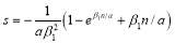
To account for the variety of targets in real life defense scenarios, we consider heterogeneous targets which have the same number of engagement opportunities but with different SSPKs.  To engage heterogeneous targets, we propose that at the first engagement opportunities, it is suitable to employ the SLS-FSS tactic since the defense does not know how many targets are coming and the fact that the SLS-FSS does not require a known number of targets.  However, through the kinematics described in Section 2, the defense is able to recognize its last engagement opportunity.  That is, if the defense does not neutralize all targets at the last engagement opportunity it will be defeated.  Therefore, it is sensible to allocate the number of interceptors in a way that the defense maximizes the at the last engagement opportunity.  We call this the SLS-OLEO (Shoot-Look-Shoot tactic with Optimal Last Engagement Opportunity).

If there is only one target then the defense will engage that target with as many interceptors as possible.  In practice, we are not suggesting that the defense launches all of the remaining interceptors against that last target but rather a number of interceptors that yield a desirable , for example .  The maximum number of interceptors launched against a target is also limited by the battle space (time and physical space available), so that each launched interceptor takes away a portion of the battle space.

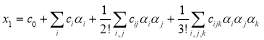
If there is more than one target then the defense has to carefully choose the allocation of interceptors against each target to maximize the .  Fortunately, this can be done efficiently by observing that the is a concave function in the number of interceptors.

5 – CONCAVITY OF THE

Concavity implies that there is an allocation of interceptors that globally maximizes the .  The proof of concavity is relatively short, can be done by induction and is shown in Appendix A.  However, to clarify the idea, we define below our notation:

1. is the against target and
2. is the Single Shot Probability of a Miss () against target.

For illustration, we show the for two targets:

          (10)

where is the number of interceptors allocated to target 1 and is the number of interceptors allocated to Target 2.

The criterion for a real and continuous functionto be concave is the inequality below (Gradshteyn and Ryzhik 1979):

        (11)

where and lie in the domain of interest.  Note that the functionis not the same as the salvo size.

Example 5A. Let the number of targets be two (), the number of interceptors be six  (), the against Target 1 be percent , and the against Target 2 be percent . Then,

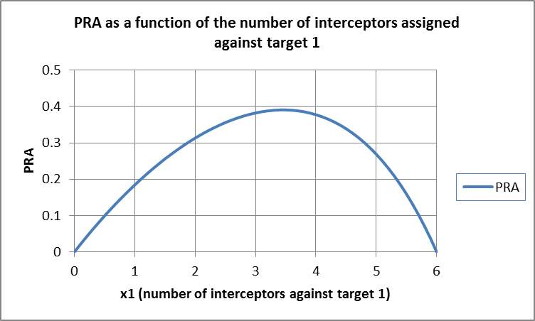
Figure 2 – is concave.

        (12)

Figure 2 displays the function from Eqn (12), which is concave over the range of interest i.e., .  Clearly, there is exactly one maximum, and thus the local maximum corresponds to the global maximum in this continuous concave function (Winston and Venkataramanan 2003).  To find the global maximum value we must determine the number of interceptors, against Target 1, which yields a zero derivative.  For a continuous solution, the maximum occurs at 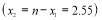interceptors, which is roughly between three and four interceptors.  For an integer solution, we can compare the evaluated at integers that are in the neighbourhood of the continuous solution.  Though it is not obvious from Figure 2, .  Therefore, assigning three interceptors against Target 1, where   (three interceptors against Target 2 i.e. ), yields the best .  We discern that the difference between these two solutions is minimal and can be approximately considered as equal in practice.

After proving the concavity of the , we discovered that it was also proven in (Bourn 2012), with a more formal mathematical approach that provides the same result.

6 – GLOBALLY OPTIMAL SOLUTION

This Section explores various solutions for optimizing the including a solution using perturbation theory, a solution using bisection, and an integer solution. We shall also provide an analysis of homogeneous and heterogeneous threats.  Perturbation provides a quick estimate of the solution as it is represented by formulae while bisection provides an accurate numerical solution.  Both techniques are shown to be consistent.  Perturbation’s solution could also be used as an initial guess for bisection.  Additionally, the fact that the is concave guarantees that there is a globally optimal solution and it can be found using bisection.  However, since the number of interceptors is an integer we will look for integer solutions surrounding the continuous solution.

First, we aim to maximize the , which presents a constrained optimization problem. However, given the concavity of the function proven above and the continuous nature examined in this section, we can use calculus to efficiently find a solution.  Thus, we will derive a function with one unknown, where solving for the unknown gives the optimal allocation of interceptors.  The we wish to maximize is:

        (13)

where 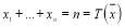.  To optimize the, calculus with constraints (Marsden and Tromba 1981) dictates that there is a such that:

          (14)

Performing the derivatives, we get for

         (15)

For example, with three targets, there are three equations (we have redefined as for convenience):

        (16)

The last equation is constrained.  That is, :

       (17)

Dividing the second equality by the first equality of Eqn (16) and using algebra, we get:

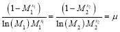
Solving for, we get:

Generalizing, we arrive at the following:

       (18)

and,

         (19)

This means that if we could solve for then we can obtain all other values through the functions and using Eqn (19).  This is indeed the case as we can divide the first equality of Eqn (17) by the first equality of Eqn (16) and simplify to obtain:

   (20)

We now observe that there is only one unknown in Eqn (20).  Due to the concavity of the objective function, there is exactly one solution for.  In general, we have to solve:

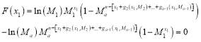      (21)

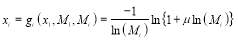
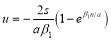
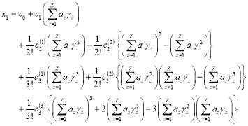
6.1 Approximate Solution using Perturbation Theory

In this subsection, we make use of perturbation theory (Simmonds and Mann 1986) to approximate as a function of the up to the third order in the parameters .  In other words, we shall use Eqn (21) to solve for :

         (22)

where and the are sorted in decreasing order i.e. so that for.  Eqn (22) is a formula which is convenient to estimate the value of .  Perturbation theory allows us to substitute the expression for in Eqn (22) into Eqn (21) and expand Eqn (21) in a Taylor’s series in the variables .  That is,

           (23)

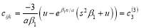
The coefficients will depend on the coefficients .  Sinceis equal to zero, we shall set s  to zeroes and solve for .  We show below the expressions for the coefficients .  For pure convenience, we must first define the parameters:

  (24)

 (25)

  (26)

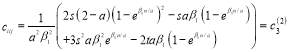
For , and , the coefficient can be written as shown below (these coefficients were obtained with the help of the software Mathematica (Wolfram 2013)):

  (27)

  (28)

  (29)

for .

  (30)

  (31)

for distinct,

 (32)

with distinct.

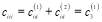  (33)

where,

 (34)

 (35)

We observe that the coefficients s are not dependent on the s.  For example, while 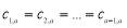.  What is more, the coefficients s are not merely numerical but analytical expressions in terms of the parameters of the problem i.e. the number of targets , the number of interceptors and  the of the first type of target (which by definition has the highest value of among all types of targets).

Example 6A. We assume the same scenario from Example 5A: there are two targets (), six interceptors (); against Target 1 is percent (), and against Target 2 is percent ().  Eqn (22) yields, hence .  Note that these results are only approximations to the true values of and.

The perturbation series in Eqn (22) can be simplified when we group the targets into identical types.  That is, each type of target has the same and the same.  Letbe the number of types of targets; the number of targets of type   and where is theof a target of type .  can now be expressed as

    (36)

6.2 Solution using bisection

Eqn (22) dictates that if all of the s are homogeneous then for.  However, if at least one of the s is different from the rest, then Eqn (22) dictates that as.  From here on, we assume that at least two of the s are different.  We also note that if   then , and so:

  (37)

Eqns (22) and (37) show that .  Due to the effects of concavity, there is only one possibility for .  In addition, we could further narrow this interval by determining the minimum integer such that .  We know that such a exists because and.   This can be done by repeatedly increasing the value of in increments, starting from and continuing until .  While incrementally increasing the value for , if then we must replace the lower bound by .  This necessitates that the value for will lie between the interval .  Note that the maximum length of this interval is one.  This is an ideal situation to use the bisection method (Press et al. 1992) to solve for.  The bisection method is a technique that finds a root once we know that it lies in a specific interval.

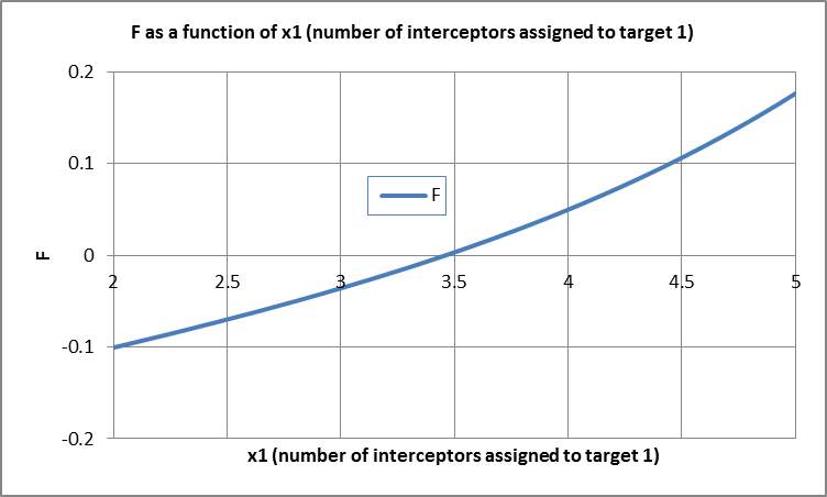
Figure 3: as a function of   (number of interceptors assigned to Target 1).

Example 6B. We again use the same scenario as the one in Example 5A, where there are two targets , six interceptors (), against Target 1 is percent, and against target 2 is percent ().  In this scenario, is plotted as a function of (the number of interceptors assigned to Target 1) as shown in Figure 3.  It is seen that is a monotonically increasing function of and crosses the x-axis exactly once at .  This corresponds to the maximum in Example 5A.  As indicated above, the bisection methodology cannot fail for a concave function such as the .  Therefore, we argue that this is a very robust solution using bisection.

6.3 Observation for Integer Solutions

We have just provided the globally optimal continuous solution to the , and can now define the boundary parameters for finding an optimal solution.  In a realistic scenario, the allocation for interceptors against a target must be a non-negative integer.  Because the is concave and the allocation of interceptors   lies on a hyperplane in dimensions , we can examine integer solutions that surround the continuous solution.

Observation 6A.  We can show that one integer solution yields a better if it is closer to the continuous solution along a line that connects the continuous solution and a feasible solution.  This holds as the is a concave function.  That is, let and be two feasible integer solutions such that where i.e., lies between and.  By concavity, we get

Sinceis the optimal solution then which implies that

This concludes the proof asis closer tothan.  Note that is a feasible continuous solution for any as

However, the integer solutionmay or may not exist due to integer values that make upas the line connectinganddoes not necessarily intersect other integer solutions beside.  Therefore, we suggest another approach in the next section.

6.4 Integer Solution that is Nearly Optimal

We propose here a suboptimal solution that is based on integers as illustrated in Example 6C.

Example 6C. We assume that there are two targets of Type 1, three targets of Type 2 and ten interceptors.  Each type of target has a characteristic: and .  For illustration purposes, we will let and.  Perturbation dictates that .  Refining using bisection yields.  The continuous optimal engagement allocation of interceptors consists of using Eqn (18).  This means that each target of Type 1 is engaged optimally with 3.056 interceptors and each target of Type 2 with 1.296 interceptors.  Observe that the optimal (continuous) allocation to each type of targets is identical which signifies that we only need to use Eqn (18) as many as the number of types of targets: twice in this example for two types of targets.  We initially assign to each type of targets the nearest integer that is below or equal to the continuous solution: interceptors against each Type 1 target and interceptors against each Type 2 target.  This means that the individual allocation consists of i.e., and 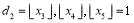.  The remaining interceptor(s) is assigned in a way that optimizes the.  That is, we choose the number of interceptors against Type 1 targets to range from to while the remaining or interceptors are assigned to Type 2 targets.  The number of interceptors are allocated as uniformly as possible among each type of targets and hence (sub) optimize the as shown in (Soland 1987).  Hence,

The above yields using Eqn (1):

which is greater than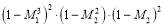.  That is, allocating the remaining interceptor to Type 1 targets produces a betterthan allocating it to Type 2 targets in this example.  This, of course, can be generalized to more than two types of targets which is when this algorithm is the most useful.  We remark that each target needs to be assigned at least one interceptor in this nearly optimal solution.  Hence, 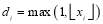for.  This evidently requires that the number of interceptors is greater than or equal to the number of targets.  Otherwise, the would be equal to zero since there would be targets that are not engaged due to the shortage of interceptors.  As shown in this example, the algorithm is efficient.

In general, we determine the suboptimal integer solution as follows:

1. Using perturbation, Eqn (22), to estimate;
2. Improving the accuracy of using bisection;
3. Using to determine other, Eqn (18);
4. Finding the greatest integers that are less than or equal to .  That is, ;
5. Making sure that there is at least one interceptor engaging each target i.e. ;
6. Allocating interceptors as evenly as possible among targets of the same type, and
7. Choosing the number of interceptors allocated to each type that maximizes the .

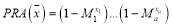
7 – Measures of effectiveness (MOEs)

The impacts of three firing tactics: Soland’s tactic, the SLS-FSS tactic and the SLS-OLEO tactic are analyzed by evaluating the and the .  We will assume that there are two targets of Type 1 and three targets of Type 2, and that  each type is characterized by a : and .  For illustration, is set to be while varies from to.

Figure 4 shows that the increases with . In comparison, Soland’s tactic provides the best as expected since it is designed to be globally optimal;  the SLS-FSS tactic provides the worst also as expected as there is no optimization; and the SLS-OLEO tactic surprisingly provides a very close to  that of Soland’s tactic.  This is very fortunate as the SLS-OLEO tactic does not assume a known number of targets unlike Soland’s tactic, which makes the SLS-OLEO more realistic and applicable in real life scenarios.  Futhermore, the improvement in the from the SLS-FSS tactic to Soland’s tactic and the SLS-OLEO could be as large as 30 percent, which corresponds approximately to a of 40 percent.

Figure 4 – as a function of , computed for Soland’s tactic, the SLS-FSS tactic and the SLS-OLEO tactic.

The improvement in the s comes at the cost measured in terms of the .  Figure 5 shows that the decreases with .  This is true as the probability of neutralizing all targets at the first engagement opportunity increases with and so there is a lower probability that requires the defense to re-engage all targets.

Soland’s tactic and the SLS-OLEO tactic provide similar s.  They consume the largest number of interceptors.  This is to be expected as Soland’s tactic and the SLS-OLEO tactic provide the greatest s.  The improvement in the s as compared to the SLS-FSS tactic is partially due to the fact that Soland’s tactic and the SLS-OLEO tactic use more interceptors than the SLS-FSS tactic (in addition to the optimization).  We note that the for Soland’s tactic does not decrease monotonically as a function of –  this feature of Soland’s tactic is not widely known but is true, and occurs because maximizing the does not necessarily maximize in Soland’s tactic even though the two MOEs are correlated (Nguyen & Miah 2015)

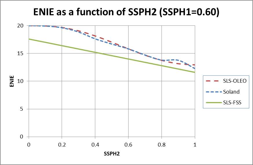
Figure 5 – as a function of , computed for Soland’s tactic, the SLS-FSS tactic and the SLS-OLEO tactic.

8 – PROBABILITY OF INTEGRATED SYSTEM EFFECTIVENESS ()

is an indicator of BMDS that can be thought of like a system of systems; or the birds-eye-view of all of the components working together, and evaluates the BMDS’s overall effectiveness. Boeing describes a probabilistic model that accounts for the high-level components of the Ground-based Mid-course Defense (GMD) system and produces an overall, quantitative measure of the effectiveness of the system called the   (Boeing Co 1999).  In a given scenario, represents the probability of negating all RVs –  for example, a value of implies that out of ten battles nine of them will defeat all RVs and one of them will have at least one leaker.

The top level of the GMD effectiveness breaks into eight system level functions that are essential to negate the threats.  The corresponding probabilities to these top-level functions are listed below:

1. The probability of system availability at the beginning of the operational period.
2. The probability that the GMD system continues to function throughout the operational period.
3. The probability that the system activates and performs all required planning.
4. The probability of processing the autonomous missile track report, and producing and communicating a sensor task plan.
5. The probability that the sensors successfully perform cued surveillance, tracking and required discrimination in support of mid-course guidance.
6. The probability that the sensors provide BMC3 (Ballistic Missile Command, Control and Communications system) with sufficiently accurate information.
7. The probability that the sensors are functional for the attack duration.
8. The based on firing doctrines.

Each of these probabilities can be obtained from lower level probabilities.  See (Boeing Co 1999) for more detail.  In absence of official data, we will parametrize them to be identical and equally important.  We further assume that their effectiveness ranges from to and denote this parameter as.  We will show that the value drops substantially when is less than.  In reality, these probabilities might differ.  However, such assumption illustrates the driving force to the value.  For heterogeneity, we also assume a typical of and of 70 percent.  Figure 6 displays the value as a function of.

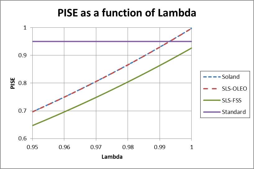
Figure 6 – as a function of for Soland’s tactic, the SLS-OLEO tactic and the SLS-FSS tactic.

Figure 6 shows that the value drops quickly when decreases.  At, is only at most 0.70.  This occurs because the system integrated effectiveness depends on a large number of critical components.  Notably, the SLS-FSS tactic will not meet the standard value of of 0.95 (Wilkening 1999) while Soland’s tactic and the SLS-OLEO tactic can meet that standard when . These numbers are significant, because any small improvement to the requires that all the components work perfectly together and at an extremely high performance.

One way to improve the value is to improve by building redundancy into the BMDS.  Another way to improve the value is to consider boost phase engagement.  It was found (Nguyen 2014) that the boost phase engagement improves the value significantly even when its probability of success of a boost phase engagement assumes a modest value such as .

9 – CONCLUSION

In this paper, we determined that during a complex engagement scenario with heterogeneous targets, the SLS-OLEO (Shoot-Look-Shoot with Optimal Last Engagement Opportunity) will optimize the defence’s (Probability of Raid Annihilation) at the last engagement opportunity.  This, in turn, contributes to the (Probability of Integrated System Effectiveness), which is itself a measure of the effectiveness of the defence’s BMDS.

To reach this conclusion, we investigated three firing tactics: the SLS-FSS tactic (Shoot-Look-Shoot with Fixed-Size Salvos), the SLS-OLEO tactic (Shoot-Look-Shoot with Optimal Last Engagement Opportunity) and Soland’s tactic.

When comparing the advantages and disadvantages of each tactic, we found that the SLS-FSS tactic generates the lowest , Soland’s tactic offers the highest and the SLS-OLEO tactic provides a similar to the one based on Soland’s tactic – which is very fortunate for two reasons: first, Soland’s tactic is designed to yield the best theoretical when the number of targets is known;  second, the SLS-OLEO tactic makes no assumption about the number of targets – which is a more realistic scenario – yet still achieves a close to the best theoretical best (Soland’s tactic).  Furthermore, when targets are heterogeneous, meaning that they have different s, there is an imminent need to optimize the by selecting the appropriate number of interceptors against each target.  This is accomplished in both the SLS-OLEO tactic and Soland’s tactic.  We argue that this comparison makes the SLS-OLEO tactic stand out as the preferred tactic for BMD.

In addition to optimizing the , we found that SLS tactics can achieve the same value as that of the Salvo tactic, but with a lower number of interceptors. Specifically, for homogeneous targets, we found that the defense typically performs equally with SLS tactics and an inventory of three interceptors per RV, as compared to the Salvo tactic and an inventory of four interceptors per RV.  For this reason, we argue that if the defense uses SLS tactics and is provided with the same inventory as it uses in the Salvo tactic (twenty interceptors in our scenario), they will have more remaining interceptors. This would result in lower costs associated with each mission.  This finding remains true for heterogeneous targets, where the defense can also reduce the number of interceptors required per RV.  In general, we found that the number of interceptors saved due to SLS tactics increases with increasing s. In comparison, we found that the SLS-FSS tactic saves the greatest number of interceptors while Soland’s tactic and the SLS-OLEO tactic provide similar inventory savings.  This is logical because Soland’s tactic and the SLS-OLEO tactic use more interceptors than the SLS-FSS tactic to generate higher s.

We also considered that the when combined with the effectiveness of the other high level components of a BMD system produces the .  The value is highly constrained by these high level components.  To achieve a value of – criterion for the NMD (National Missile Defense) system, (Wilkening 1999), each of these components’ effectiveness must be at least assuming that their effectiveness are equal.  For this reason, we suggest two ways to improve the value: to build in redundancy in the GMD/NMD system and to consider boost phase engagement.

The implementation of the first proposal to improve the would be very costly, as it requires a duplicate GMD/NMD system.  Cost aside, the effectiveness of high-level components would be significantly improved, creating a substantial increase in the value.  The implementation of the second proposal would be difficult to achieve due to technological challenges, that is, the interceptors must have very high speed and accuracy in order to engage threats in boost phase.  Such challenges might be met if the GMD/NMD components are located nearby the RV launch sites. Despite this complication, the value improves significantly even for a very low rate of success in the boost phase engagement, making the boost phase engagement a promising option.

In future research, the concavity of the which was proven in this paper, could have other applications. Our calculations presented in Section 4 may therefore also be used to optimize functions that are similar to the , such as the objective function of a search and detection mission as one example. In addition, there is also the possibility that other calculations presented in this paper could be extended in more general terms. For instance, instead of calculating OLEO (Optimal Last Engagement Opportunity), one could calculate for OREO (Optimal Remaining Engagement Opportunities). In OREO, the calculations would include any remaining opportunities; for example, once the number of remaining opportunities to intercept various targets is known, there is a possibility for staggered calculations and further adjustment. An example scenario would be if there are five incoming missiles, all launched at slightly varying times and travelling at different speeds. Once the defence is aware of how many chances to intercept each target, it can adjust its calculations to maximize the for all targets over multiple remaining opportunities for interceptions – rather than only at a single, or last engagement opportunity.

In summary, we have provided a comparative analysis of various firing tactics, and optimized the (Probability of Raid Annihilation) to enhance how many successful hits the defence can make in a realistic engagement scenario. This analysis allows us to better understand the resulting (Probability of Integrated System Effectiveness), which provides insight into the overall effectiveness of the defence system.  In contrast to the existing body of literature on this topic, our parameters included heterogeneous, as opposed to homogeneous, targets. We believe that this reflects the conditions of a more realistic engagement scenario, and hope that this consideration enhances the practical usability of our calculations.

References

Al-Mutairi, D. K.., R. M Soland. 2005. Attrition through a partially coordinated area defense. Naval Research Logistics. 52 74-81.

Boeing Co. 1999. Appendix B – Integrated System Effectiveness Model.

Bourn, S. 2012. Probabilistic Shoot-Look-Shoot Models. PhD Dissertation, School of Mathematical Sciences, University of Adelaide, Australia.

Garrett et al. 2011. Managing the Interstitials: A System of Systems Framework Suited for the Ballistic Missile Defense. System of Systems Engineering. 14  87–109.

Brown et al. 2005. A Two-Sided Optimization for Theater Ballistic Missile Defense. Oper. Res. 53 745-763.

Dou, J., J. Yu and F. Long. 2010.  Research on Anti-Ship Missile Saturation Attack Problem.  Proceedings of the 2009 International Conference on Mechanical and Electronics Engineering. 31-36.

Gradshteyn, I. S., I. M. Ryzhik, 1979. Tables of Integrals, Series, and Products. Academic Press. San Diego, CA. 6^th Ed. 1100.

Holland, O. T., S. E Wallace. 2011. Using Agents to Model the Kill Chain of the Ballistic Missile Defense System. Naval Engineers. 123 141–151.

Karasakal, O.  2008.  Air defense missile-target allocation models for a naval task group.  Computers & Operations Research 35, 1759 – 1770.

Karasakal et al. 2011.  Anti-ship missile defense for a naval task group.  Naval Research Logistics. 58 305-322.

Burk, R., B. Foote. 2009. A Preliminary Analysis of Loitering Aircraft as a Capability Added to Theater-Level Anti-Ballistic Missile Systems. Military Operations Research 14 5-18.

Cranford , K.  2004. Battle Area Region Threatened Model (BART).  NORAD-USNORTHCOM/AN (North American Aerospace Defense Command – United States Northern Command/Center for Aerospace Analysis) Version 5.3.4x. and the CheckThreats subroutine.

Glazebrook, K., A. Washburn. 2004. Shoot Look Shoot: A Review and Extension. Operations Research. 52:3 454-463.

Marsden, J. E., A. J. Tromba. 1981. Vector Calculus. 217-224.

Menq et al. 2007. Discrete Markov Ballistic Missile Defense System Modeling. European Journal of Operational Research. 178 560–578.

Nguyen, B. U. 2014.  Assessment of a Ballistic Missile Defense.  Defense & Security Analysis. 30:1 4-16.

Nguyen et al. 1997. An Engagement Model to Optimize Defense Against a Multiple Attack Assuming Perfect Kill Assessment.  Naval Research Logistics. 44 687-697.

Nguyen, Bao and Suruz Miah.  Comparison of metrics for missile defence between perfect coordination and no coordination, DRDC Scientific Report (SR) DRDC-RDDC-2015-R228, Oct 15.

Nguyen, Bao and Suruz Miah.  Analysis of maritime air defence scenarios,  IEEE symposium on computational intelligence for security and defense applications, Dec 14.

Press, W. H. et al. 1992. Numerical recipes in Fortran 77  (The Art of Scientific Computing). Cambridge University Press. 2nd Ed. 343-347.

Simmonds, J. G. and J. E. Mann. 1986. A first look at perturbation theory. Robert E. Krieger Publishing Company. 2nd Ed. 6-8.

Soland, R.M. 1987. Optimal Terminal Defense Tactics when Several Sequential Engagements Are Possible.  Operations Research. 35537-542.

Vallado, D. 2001. Fundamentals of Astrodynamics and Applications.  The Netherlands: California and Kluwer Academic Publishers. 88-103, 445-447.

Washburn A. 2005. The Bang-Soak Theory of Missile Attack and Terminal Defense. Military Operations Research Journal. 10:1 15-24.

Weiner, S. D. and S. M. Rocklin. 1994. Discrimination Performance Requirements for Ballistic Missile Defense.  The Lincoln Laboratory Journal. 7:1.

Wilkening, D. A. 1999. A Simple Model for Calculating Ballistic Missile Defense Effectiveness. Science & Global Security. 8:2 183-215.

Winston, W. L. and M. Venkataramanan. 2003. Introduction to Mathematical Programming.  Brooks/Cole, 673-678.

Wolfram. 2013. Mathematica 9. Wolfram Research Inc.

Yossi A., M. Kress. 1997. Evaluating the Effectiveness of Shoot-Look-Shoot Tactics in the Presence of Incomplete Damage Information.  Military Operations Research Journal. 3:1 79-89.