Abstract

The bone growth analogy is the bone’s ability to adapt to the level of stress it feels by either growing in cross-section or deteriorating in size when under-stressed. The potential to utilise an organic optimisation procedure within steel constructions is explored in this research work, with focus on achieving material savings and hence reducing carbon emissions. Isolated examples of using stress optimisation in small-scale productions are acknowledged, however a gap in knowledge is identified in designing more evenly stressed steel structures. Combined with the construction industry’s practice of using constant standard beam sections, potential for reducing structural weight is further underlined.

The organic optimisation procedure has been utilised to define a bone decay analogy firstly in steel cross-sections by discretising the section into a mesh and progressively removing redundant material. By recalculating principal stresses after each iteration loop, the section converges into its most optimal form, where the maximum stress is just below the material capacity. Two boundary conditions have been introduced in the study, material continuity and a constant flat top for constructability reasons. Throughout the research work, a design example with a common loading condition has been used to design for loading in the major axis as well as biaxial case.

When analysing for a single cross-section, the most efficient shape emerges to be an I-beam for loading in single axis and a box-section for two-directional loading. The thickness of the flange varies accordingly to the level of stress experiences, with the web remaining at a constant predefined minimal thickness, proving that any shear effects are negligible. It is noted that the level of optimisation achieved is dependant on choosing an appropriate iteration step size.

By extruding singly optimised beam sections into a long span, the most efficient beam section is achieved. Employing the most critical section already improved to the bone decay analogy, two alternative procedures for developing an efficient beam are further defined. The first optimises for section height with the other for a varying base flange breadth. All three methods are compared to material usage in comparison to a constant section geometry, serviceability, constructability and embodied carbon. All three design solutions have proved to remain within acceptable deflection limits with the bone decay analogy emerging as the most efficient solution, saving up 21% of material weight in contrast to a uniform section. Calculating for a varying height proved most beneficial in the case of bi-axial loading, saving 16% of material in comparison to 10% for singly loaded beam. Only in the case of loading in the major axis, an analysis for varying base width was conducted, resolving in a section 16% lighter than the original.

Admittedly, manufacturing steel sections with varying flange thicknesses to an industrial scale has remained a novelty, however 3D printing is constantly proving to provide scope for producing highly customised solutions. Within currently accessible production technology, a beam with varying height or flange width are the most attractive design solutions, reducing steel carbon emissions by a considerable amount. Ultimately, it has been proved that by discarding redundant material from a steel structure, a more evenly stressed and lighter steel section can be achieved. Finally, the dissertation then suggests multiple avenues that the research could go down in the future in terms of reaching further savings in material, covering larger structures as well as undertaking design verification.

List of symbols

A  Total area of shape Ai  Area of element Asi Area above cut line b Maximum breadth of cross-section c Number of cuts considered E Elastic or Young’s Modulus of steel f Thickness of top flange h Maximum height of cross-section I  Second moment of area L Length of beam M1  Moment in major axis M2  Moment in minor axis Me  Elastic moment capacity P Axial force S  Shear force S1 Shear force in major axis S2 Shear force in minor axis t   Length of cut line wt Thickness of web w1 UDL in the major axis w1SLS  Serviceability limit UDL on major axis w2 UDL in the minor axis x Location along the beam yi  Height from datum to centroid y̅ Level of neutral axis τ  Shear stress σ  Bending stress σmax  Material stress capacity σp  Principal stress σ1  Major bending stress σ2  Minor bending stress δ Deflection of beam

List of abbreviations

3D Three Dimensional

AM Additive Manufacturing

BESO Bio-directional Evolutionary Structural Optimisation

ER Evolution Rate

ESO Evolutionary Structural Optimisation

FE Finite Element

GA Genetic Algorithm

MES Minimum Effective Strain

RR Rejection Ratio

SLS Serviceability Limit State

TO Topological Optimisation

UDL Uniformly Distributed Load

ULS Ultimate Limit State

1         Introduction

Bones are able to adapt to their environment by growing when over-stressed and decaying in cross-section when under-stressed. Thanks to this ability, bones are a near-optimum structure tailored to their specific external loading.

The construction industry has great potential to learn from this method of organic optimisation. While it is known from basic structural analysis that the actions experienced by a structural beam are not uniform in magnitude along its length, standardised hot-rolled steel sections are still most widely used in industry as the basic steel skeleton of a building. This conservative approach, where sections are sized based on the most critical stress that the member will experience along its whole span provides consistent structural capacities, however rendering the majority of the length to work well below its capacities.

Applying the bone decay analogy in steel beam design holds opportunity to lead to a much more evenly stressed structures, with the steel sections tailored to the loading it is under. Nowadays custom steel sections are mainly only used in design situations where the level of stress experienced is outside the bounds of standard sized members, or as an architectural statement by exposing the refined steelwork to highlight structural honesty (Meyer Boake, 2015). Such bespoke steel design solutions have remained a novelty and are economically viable only in high-end design projects.

Custom designs are significantly more expensive than utilising industry standard section, which is why for low budget projects, the incentive to design more efficiently working custom steel members might be lost. However, as the industry gains expertise and bespoke production technologies become more affordable, the sift towards optimised design solution is no longer out of grasp. In parallel to the construction industry’s effort to reduce carbon emissions and to use construction material more efficiently, the aim of this research project is to analyse the viability of the bone decay analogy on steel member design and to develop sets of more evenly stressed and therefore more efficient beam sections that would respond to common loading scenarios.

1.1    Scope of project

Firstly, existing literature on recognised structural optimisation methods are investigated and exemplified with case study findings. Precedents on using optimisation software on small-scale design projects such as structural node design are discussed, however a gap in knowledge is identified in the optimisation of steel loadbearing members.

The programming software Python has been used to develop an algorithm to identify and remove under-stressed material, following the bone decay analogy, until an optimum solution is achieved. Throughout this study, a simply supported beam of a 7×7 grid with standard loading has been used as a design example. The bone decay analogy is applied firstly on a single cross-section under uniform loading in the major axis, as well as under biaxial loading. Following on, possible pitfalls within the optimisation procedure are identified and boundary conditions for constructability are defined. Furthermore, applying the identified boundary conditions, the bone decay analogy is expanded from a single cross-section to a whole beam profile. Two further methods, one with a changing section height and another with varying base breadth are developed as variations to the pure bone decay analogy.

Throughout the research project, the design example of the simply supported beam under uniform loading condition has been utilised in order to be able to draw valid comparisons between the resulting designs of the three optimisation methods. Taking into account the amount of material used, serviceability limits and constructability, the three approaches are compared to one anther in order to deduce the closest to optimum and most realistic method. In conclusion, the benefits and drawbacks of the developed bespoke beam profiles are compared to that of the industry standardised steel sections, encouraging further research in the area.

2         Literature review

The following literature review aims to place the research work in content by firstly defining the bone growth analogy and illustrating it with examples. Further on, studies into the recognised methods and possible pitfalls of optimisation will be investigated. Lastly, the constructability of custom optimised sections will also be analysed.

2.1    Bone growth analogy

Bones grow when they are stressed and decay as they are under-stressed, thereby constantly adapting to their loading environment. This is the reason as to why one needs to keep exercising when recovering from a broken bone for medical reasons, in order to avoid any further loss in bone structure (Burgoyne, 2007).

This rule was first defined by Frost in 1964 as the Minimum Effective Strain (MES) theory, stating that strains below the MES do not evoke adaptive architectural bone modelling, while those exceeding it do (Frost, 1964). The hypothesis has since achieved experimental support, showing that bone material has the ability to respond to changes in its mechanical loading environment (i.e. change in the stresses and strains), by adapting its shape and/or its internal micro-structure with the two aspects commonly referred to as surface and internal remodelling, with an example to follow (Frost, 1983).

2.1.1     Example 1: Rib cage adaption

Saumarez (1986) set to investigate the human upper rib cage in order to analyse the actions of the intercostal muscles. The rib cage was modelled along the length of its cross-section with a system of forces acting upon it. Moving along the rib-bone, it became clear that the changes along the cross-section, together with any grooves, followed the pattern of forces along the rib. By interpreting the computed moments at each cross-section and comparing the specific loading conditions along the length of each rib, it was concluded that each cross-section was the near optimum shape to the loading it was subjected to (Saumarez, 1986).

For instance, where the rib was bent maximally about its lateral axis, its cross-sectional shape was roughly a “T”, which is a conventional engineering cross-section for beams that have to withstand bending about one axis. This is as shown in cross-section 2, in Figure 2.1.1 below. Therefore, following the hypothesis raised by Frost, it was proved that as a result of the bone’s capacity to accommodate for the forces it is subjected to, the human rib cage has grown to become optimally light and efficient (Saumarez, 1986).

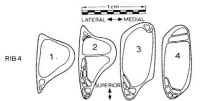
Figure 2.1.1 Cross-sections showing the organically optimised human rib cage (Saumarez, 1986)

2.2    Optimisation methods in structural design

When material is added at a point in a loaded optimal structure, the stresses will fall, however, the added material has not contributed to the strength of the structure, but merely to its weight. Conversely, if material were to be removed from the same point considered in the ideal section, the stresses will rise to exceed the section strength and the structure will fail (Saumarez, 1986).

Several methods of optimisation have been developed in order to reach the desired optimum state as defined above. The usual optimisation problem is set out by defining what is to be optimised, together with any boundary conditions to be applied. In structural design, most problems commonly minimise volume for maximum stress, with some of the most widely utilised methods including the Genetic Algorithm (GA), Floating Point Arithmetic and the Ant Colony Optimisation theory. These are mathematical models involving a higher degree of modelling, set out to achieve construction savings and minimal structural weight (Kikuchi and Horimatsu, 1994).

2.2.1     Evolutionary Structural Optimisation (ESO)

An optimisation method closely following the bone growth analogy was first defined by Xie and Stevens (1992) as the Evolutionary Structural Optimisation (ESO) method. The proposed ESO method aimed to mimic an evolutionary process where material defined as under-stressed is progressively being eliminated from the structure (Xie and Steven, 1992).

The method utilises the Von Mieses yield criterion in order to eliminate elements with internal stresses less than a pre-defined Rejection Ratio (RR) times the maximum Mieses stress over the structure. This cycle has been repeated until a steady state is reached, after which an Evolution Rate (ER) is introduced and added on to the RR, repeating over the iteration. The level of optimisation reached is dependent on how refined the RR and ER are. For example, the same problem can reach a closer to optimum state when a smaller evolutionary state is defined, as it will result in many more optimisation cycles (Xie and Steven, 1992).

2.2.1.1       Example 2: Bone decay

Figure 2.2.1. Metal implant embedded in bone illustrating optimisation precedure from original section to RR=1%, finalising at RR=10% (Xie and Steven, 1992)

Using the introduced ESO method, Xie and Steven further went on to model an example of natural evolutionary structural optimisation, when metal implants are used to repair broken bones. It has been noted by medics how metal implants can actually have a deteriorating effect on the recovery of the bone structure. Being much stiffer, the metal implant is working hardest, with the bone itself actually not being sufficiently stressed, resulting in part of the bone to diminish as calcium is absorbed into the blood stream (Xie and Steven, 1992).

A Finite Element (FE) model of a metal implant embedded in bone, illustrated in Figure 2.2.1, was produced. Using the ESO method, it was shown how the structure followed the Minimum Effective Strain theory set out by Frost in 1964, and how the bone indeed started diminishing in cross-section as material was under-stressed (Xie and Steven, 1992).

2.2.2     Bio-directional Evolutionary Structural Optimisation (BESO)

Since the initial publication of the Evolutionary Structural Optimisation theory in 1992, extensive research on the topic was done, with the core authors publishing many more papers as well as a book on the evolutionary method (Xie and Steven, 1997). The ESO method has further been proved to resolve a full range of structural optimisation problems, however suffering from a few major deficiencies, namely solution time and uniqueness. Therefore, it was pointed out that in order to reach a true optimum, a bidirectional algorithm should be developed in order to be able to search all directions, by not only removing under-stressed material, but also adding material in order to alleviate high stress (Querin, Steven and Xie, 2000).

Therefore a further improved version of the ESO method was developed (Querin, Steven and Xie, 1998), aiming to allow for a more through search of all the design space in order to reach a global and not only local optimal minima. The new and advanced method was called the Bio-Directional Evolutionary Structural Optimisation (BESO), again utilising the Von Mieses stress. An example was presented where a structure with a minimum member thickness was modelled to connect the two supports as a boundary condition, applying the BESO method. As a result, computational time was significantly saved, also resulting in a self-designing structure (Querin, Steven and Xie, 1998).

2.2.2.1       Example 3: Femoral head bone

The BESO growth algorithm has been further applied on many other problems (Eschenauer and Olhoff, 2001). For instance, by defining a design domain and discretizing it by means of finite elements, a density distribution can be achieved that accounts for influences from loading and support conditions. In the study shown, presented in Figure 2.2.2, a growth under stress example was modelled on the femoral head bone. As concluded in the study, the theoretical model and calculations produced results very similar to the distribution derived from X-ray photographs, thereby further validating the BESO method.

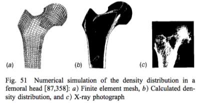
Figure 2.2.2. The femoral bone head BESO model (left) with calculated density distribution (middle), closely resemble the real bone structure (right) (Reiter, 1996)

2.2.3     Praise and criticism

The results from the above defined evolutionary optimisation methods are inherently subject to some risks, stemming from their highly computational nature. Some are analysed by Adeli and Karim (1997), on the basis of modelling cold-formed steel beams. The paper highlighted how results from a computational program based on C++ depended on from which end the calculations started, often converging into different solutions (Adeli and Karim, 1997).

A reoccurring theme amongst optimisation problems is how to correctly define the rejection criteria. This has been noted in studies for the genetic Algorithm (GA) method where it was stressed that care needs to be taken when setting the penalty functions as too strict ones may cause a failure in including a number of design families, thereby possibly excluding the most optimum solution (Jenkins, 1991).

This issue has been proved to be relevant also in the case of ESO, where studies have shown that the ESO rejection criteria may result in a highly non-optimal design. Zhou and Rozvany (2001) showed that ESO’s advantage of having conceptual simplicity also suffers from being an intuitive method with no proof of optimality. An example was outlined where following BESO, the optimisation method would add more material to an element being analysed. For the purpose of the example, the element has been removed all together instead, giving a greater than ten times closer to optimum solution than the BESO algorithm. The paper highlights several attempts at rebuttal to the stated issue, suggesting for further improvements on the method to emerge in the near future (Zhou and Rozvany, 2001).

Critics of the ESO method have further dismissed it as inefficient and lacking rationality (Rozvany, 2009). By referring to the issues explained in the 2001 paper, of at times producing unreliable and chaotic results, Rozvany (2009) claims the ESO method to lack the level of sophistication present in competing methods. He concluded that these are some of the many reasons as to why ESO is hardly used in industry applications.

Although criticised for its simplicity, the ESO method has also been praised for its intuitive nature and the possibility to know every stage of the shape and layout path towards to true optimum. During the evolutionary process, the material properties of the rejected elements are assigned as zero, further eliminating the need to generate a new mesh. What is more, in spite of being dismissed as hardly of in the manufacturing industry, the evolutionary procedure is in fact presented as a rough guide for the engineer, encouraging the use of existing shape optimisation codes in order to provide detail of the shape and size of structure. It has also been stated that although the process appears to be trivial, the results agree remarkably well with solutions obtained by analytical and other mathematically rigorous procedures (Xie and Steven, 1992).

2.3    Constructability

The capacity of the construction industry to produce highly-customised elements is rapidly improving. As a traditional approach, variations on standard cross-sections can be achieved via cutting and welding common sections or plates. Furthermore, hot-rolling can provide modified sections including tapered, castellated and curved beams (TATA, 2016).

As an exciting potential for producing bespoke elements, 3D printing is becoming a household name in the construction industry, with many studies into the structural use of 3D printed elements being undertaken. Stemming from the ability to produce highly aesthetic and customised sections, 3D printing has mostly found use in high-end institutions, however, being a time-consuming and expensive design process, the technique’s feasibility on relatively small-budgets is currently still questionable (Crolla and Williams, 2014). While the expertise and technology for 3D printing itself is expected to prevail as an expensive skill, Crolla and Williams (2014) positively predicted the raw cost of 3D printing to decline soon as many patents are to expire.

2.3.1     Topological stress optimisation

To find the most optimum design it is difficult to rely purely on engineering intuition, this is why mathematical models have been set up to iteratively solve the problem (Verbart, 2015). The Topological Optimisation (TO) method aims to find the strongest structural solution by optimising material layout within a given space to predefined boundary and loading conditions by using non-linear techniques such as GA (Sigmund and Maute, 2013). TO has found application in several industries, notably the automotive and aviation industries, where structural material savings can directly be linked to smaller fuel consumption. However, as already noted by Rozvany (2009), these methods are used in initial design stages where the designed has to further go through many further iterations to smooth out local stress failures, resulting in a produced solution far from the initial optimum. In addition to companies developing in-house software, there is a variety of open-source TO tool available, such as the Millipede and Monolith plugins, with the latter specialised in 3D printing (Monolith, 2017)(Michalatos and Kaijima, 2017). Both have been developed as components for Grasshopper 3D, a parametric design tool widely used in modern day architecture offices (Davidson, 2017).

2.3.1.1       Example 4: 3D printed node

There are some small-scale precedents to removing under-stressed material from a steel element in the design process. Utilising Additive Manufacturing (AM), research on possible node designs was carried out by Arup, the international multi-disciplinary engineering firm (Galjaard et al., 2015). The project focused on optimising a traditionally fabricated node element by using parametric design and FE analysis, in order to reduce the self-weight of the connection. The final optimised node was 75% lighter than the original, reducing the whole weight of the structure by 40%. Although the project was a success in that sense, the team also outlined a number of difficulties, including the lack of high-level computational skills combined with a vacuum of available relevant design software.

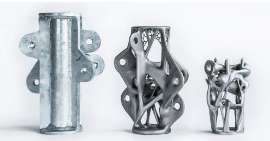
Figure 2.3.1. Model of a traditional welded node (left) with the two optimised 3D printed produces (Galjaard et al., 2015)

2.3.1.2       Example 5: 3D printed pedestrian bridge

In October 2015, a fellow Dutch company MX3D officially kick-started the project of manufacturing a steel 3D-printed pedestrian bridge, to be planted at the heart of Amsterdam’s red light district (MX3D, 2017). By customising multi-axis robots, normally used in the automotive industry, with steel welding nozzles the theoretical opportunity to weld infinitely large structures to a high speed is achieved. The printer is programmed to produce its own support panel and by moving along the length of the structure, the technique has opened up opportunity to 3D print on-site with minimal supervision. However due to health and safety constraints, the 8m spanning bridge is planned to be compositely printed in the company’s studio to then be transported and craned on site. With completion planned by the end of the year 2017, the pedestrian bridge would become a pioneering project and serve as an opportunity to further perfect and analyse structural 3D printing techniques as well as to develop a library of software for future projects. What is more, it would be one of the first examples of large-scale metal structures developed using stress topology optimisation software.

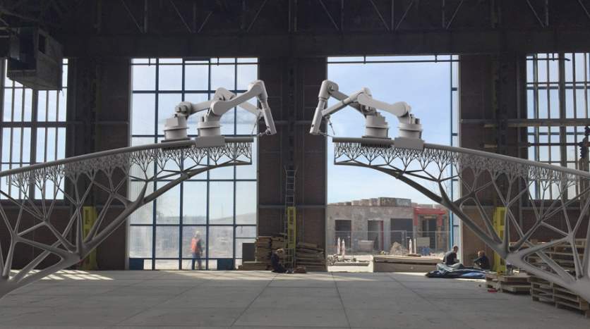
Figure 2.3.2 Visualisation of the bridge being 3D printed in MX3D’s studio (MX3D, 2017)

2.3.2     Future potential in 3D printing

Further to the previous example, 3D printing optimised elements has been proved to result in significant reductions in the weight of material being used. A study in 2014 was carried out using 3D printed customised nodes on a timber structure by producing optimised standardised sections available to be utilised in a range of situations (Crolla and Williams, 2014). It was shown that both topological optimisation for structure and other optimisation processes directly related to the manufacturing process allow for material and weight reduction of up to 60 per cent.

However, it has been pointed out that the minimum weight design often is not the most economical design. The optimisation procedure often results in a variety of customised section types for each design condition, leading to high fabrication costs (Adeli, 2000). This was also pointed out by the Arup team in their study, with the custom 3D printed elements becoming a relatively expensive part of the project, putting its economic feasibility into question (Galjaard et al., 2015).

What is more, metal 3D printing has yet to reach the capacity to produce large-scale high-strength elements. The commonly used 3D printing technique of direct metal laser sintering selectively melts and fuses metal powder with lasers in a layer-by-layer approach. It has been proved how the layer-by-layer manufacturing could lead to significant anisotropy in strength and ductility, due to poor bonding between material layers, limiting the efficacy of the printed parts (Mueller, 2016). However, 3D printing as a field is undergoing rapid development with methods already proposed to overcome the current limitations. For example, Stress Line Additive Manufacturing (SLAM) is currently under development, aiming to significantly improve the structural performance of 3D printed elements. Using a robotic arm to deposit material along three dimensional lines of principal stress, the SLAM method ensures material connectivity in the most critical direction (Tam, Coleman and Mueller, 2015).

2.4    Literature review conclusion

The bone growth analogy is an already-recognised theory with the principle being used in several optimisation methods. Although studies have shown ESO to suffer from some critical drawbacks, the simple idea of removing under-stressed elements in order to achieve a more optimum structural solution has proven to generally be a success. Furthermore, its inherent simplicity and ease of grasp make the evolutionary optimisation method stand out from highly mathematical alternatives.

What is more, when setting up the structural optimisation problem on the basis of minimizing structural weight under stress constraints, the boundary conditions should be defined with utmost care. It is important to further define realistic limits to what is actually achievable in fabrication, such as setting a minimum steel thickness. In addition to traditional approaches of welding and fabrication, 3D printing shows great potential and future capacity to be able to effectively produce bespoke structural steel elements.

3         Methodology

In order to develop an algorithm to produce the most optimum steel structure, the problem is approached in stages. Throughout the design procedure, an optimal cross-section is defined as one where the removal of any further material would result in stresses exceeding the material’s stress capacity (Saumarez, 1986). Firstly, an optimisation procedure for a single cross-section with a pre-defined loading condition is developed. Further on, the method used in designing a single cross-section is expanded for the design of a beam by dividing the span up to even length elements, calculating the forces acting at each slice and extrapolating the resulting near-optimum cross-sections to meet as a long beam. Lastly two more variations on the bone decay analogy are developed.

The optimisation program is written in Python, a high-level general use programming language (Python, 2017). Being a well-recognised software, Python is chosen both for its user friendly interface, large range of resources as well as compatibility with other software packages used in the engineering industry, including Rhinoceros and Microsoft Excel (GhPython, 2017).

3.1    Design parameters

In order to achieve consistency in the analysis, the same simply supported beam of 7m length is designed for throughout the examples, with exceptions noted. The geometry, loading, iteration and design parameters are as listed in the table below and further explained in following sections. Here the loading is based on a 7x7m grid under a 5 kN/m² live and 2 kN/m² combined dead and imposed loads, which have been factored to sum as 49 kN/m for serviceability limit state (SLS) and 71 kN/m for ultimate limit state (ULS) design load. An axial loading of 0.1 kN is applied and for biaxial loading a 40 kN/m out of plane load is designed for.

Table 2.3.2.1 Variables used in beam design

Geometry	Loading
L  = 7000 mm h  = 500 mm b  = 500 mm f  = 4 mm wt  = 4 mm	w1  = 71 kN/m w1SLS  = 49 kN/m w2  = 40 kN/m P  = 0.1 kN
Material Properties	Iteration parameters
σmax  = 275 N/mm2 E  = 210 000 N/mm2	c  = 10 RR = ER = 1%

 

3.2    Optimal cross-section design

As discussed earlier, bones have the ability to adapt to the stress state they are under by growing in cross-section if over-stressed or decaying when under-stressed. In this study, the bone decay analogy is applied by only removing material in the least stressed points of the cross-section, until an optimum solution is achieved.

The analysis can be tailored to any cross-sectional height (h) and breadth limit (b) as well as the material’s stress capacity (

σmax). Different initial sizes were tested and a 500×500 section was chosen as most practical due to reasons discussed in the results, with a maximum stress limit as 275 kN/mm² considered for steel. To design a single optimised cross-section, the axial load (A), shear force (S) and major and minor bending moments (M₁ and M₂) acting at the section will also be defined. From here, the cross-section is discretised into a mesh and maximum principal stresses as well as the axial stress for all elements of a full hxb cross-section are found. The stresses are then compared to the predefined maximum stress limit to ensure the cross-section is not overstressed and superfluous material will progressively be removed according to the bone decay analogy. As the cross-section will change in shape when material is removed, the new geometrical properties and stresses are recalculated within the calculation’s function and the process of removing material will be repeated until the cross-section converges into and optimum cross-section, as illustrated in Figure 3.2.1 below. Each step is further explained in the following sections.

Figure 3.2.1 The iteration loop visualised, showing how material is removed and stresses recalculated at each step until an optimum is reached.

3.2.1     Meshing

Based on the dimensional limits for height and breadth, a rectangular cross-section is produced and discretised into a mesh of hxb square elements, as seen in Figure 3.2.2. It is possible to refine the mesh by further dividing up the square elements, thereby giving more accurate results of the expected stress levels. This could be utilised when designing small steel elements where 1mm steps are relatively large in comparison to the member size. However, a finer mesh also brings along a delay in the iteration process as more mesh element need to be analysed, meaning the run time of the program will grow exponentially as the mesh gets smaller. For the purpose of this study a mesh accuracy of 1mm² is used.

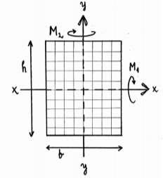
Figure 3.2.2 Cross-section of hxb size discretised into a mesh

3.2.2     Calculations’ Function

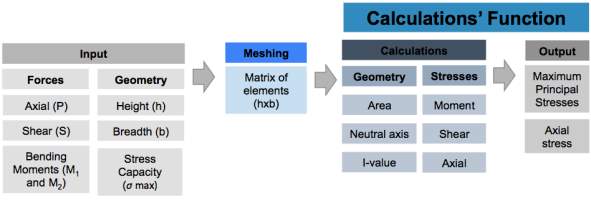
A function has been set up to calculate the maximum principal stresses and axial stresses for any cross-section based on the defined parameters. Using the dimensional limits and forces acting, the geometrical properties and stresses in each mesh element are calculated as explained in the following paragraphs. The process is illustrated in Figure 3.2.3, where the maximum principal stresses and axial stress on the cross-section are remembered.

Figure 3.2.3 The calculations’ function takes the input, creates a mesh and produces an output based on series of calculations

3.2.2.1       Geometry

In order to calculate element stresses, one needs to first know the geometrical properties of the section. The total area of the cross-section, the neutral axis location and second moment of area for any arbitrary shape are calculated as below, from the geometry of the section.

A= ΣAi

(1)

Where A = Total area of shape and A_i = Area of element

y̅=ΣAiyiA ̇

(2)

Where

y̅= Level of neutral axis, A_i = Area of element, y_i = Height to element centroid from datum line and A = Total area of shape

I=ΣAi(yi2)

(3)

Where I = Second moment of area, A_i = Area of element and y_i = Height to centroid from datum line

3.2.2.2       Stresses

Based on the cross-section geometry, stresses in each element of the mesh are calculated from the known loading condition. This includes finding the shear stress, axial stress, major and minor bending stresses as well as maximum principalstress. It is ensured that the absolute maximum principal stress will be retrieved in this step, as common programming software by default only retrieves the positive value of the square root (Langtangen, 2011). All the aforementioned stresses are calculated as follows.

τ=SΣ(Asiyi)It

(4)

Where τ = Shear stress, S = Shear force, A_si = Area above cut line, y_i = Height to centroid from datum line, I = Second moment of area and b = Length of cut line

σ=ΣMyiI

(5)

Where σ = Bending stress, I = Second moment of area, y_i = Height to centroid from datum line and M = Moment acting on section

σp=σ1+σ22 +-(σ1-σ22)2+τ2

(6)

Where σ_p = Maximum principal stress, σ₁ = Major bending stress, σ₂ = Minor bending stress and τ = Shear Stress

σa=PA

(7)

Where σ_a = Axial stress, P = Axial load, A = Area of section

3.2.3     Comparison

The maximum principal and axial stresses retrieved from the Calculations’ function are compared to the predefined material stress capacity. If the initial stresses from the full hxb cross-section already exceed this limit, the analysis will not commence and loading or dimensional limits will have to be revised to avoid section failure. If no elements exceed the stress limits, the cross-section will be allowed to enter the iteration loop, where a bone decay analogy will be implemented.

3.2.4     Bone decay analogy

In the bone decay analogy stage, under-stressed material will progressively be removed, by assigning the element stress as zeroin the principal stresses matrix. By doing so, the initially defined element matrix can be recycled until the end of the iteration process, removing the need to re-mesh the element matrix. However, some material may still be desirable to have even when under-stressed, therefore to ensure constructability, boundary conditions are implemented for reasons explained in the results, in chapter 4.2.1.

3.2.4.1       Defining under-stressed material

Here a process similar to ESO (defined in chapter 2.2.1) is introduced, where material is sequentially removed from a cross-section when under-stressed (Xie and Steven, 1992). Firstly, a Rejection Ratio is defined to eliminate elements that have stress levels lower than the RR times the material’s stress capacity. After each iteration, the RR is increased by an Evolution Rate and surplus material will again be removed. For example, if RR=1%, ER=1% and

σmax=275 kN/mm², then all elements where stresses are below 1%*275= 2.75 kN/mm² will be removed in the first iteration. The rate of iteration is to be increased by ER in each subsequent round, therefor in the second iteration loop all elements with stress below (1%+1%)*275 = 5.50 kN/mm² will be deemed as redundant and discarded.

As already noted in the case of ESO, the level of optimisation reached is dependant on how refined the RR and ER are (Xie and Steven, 1992). In order to achieve accurate results, it is imperative to undergo a step sensitivity study for each design, to confirm that the outcome is independent on the step size chosen, for reasons further discussed in section 4.2.2.

3.2.4.2       Applying boundary conditions

To ensure the practical constructability of the optimised cross-section, boundary conditions to material removal need to be set, with two introduced in the scope of this study. Firstly, the top of the sections is to always be flat and secondly, all material has to be connected. The first condition of a flat top flange is achieved by not allowing any material to be removed from the first top f rows of the section, even if under-stressed. In order to achieve material continuity, a web of a pre-defined thickness w_t is also introduced. These will be further explained and exemplified in the results section.

3.2.5     Convergence

By removing insufficiently stressed material, the remaining cross-section is forced to carry relatively more loading, which is why the geometry and stresses in each new shape need to be re-calculated. This iteration loop is repeated until an optimum shape is achieved, defined as a state of stress where the removal of any more material would cause the remaining material to work harder and finally result in exceeding the predefined strength. Once this occurs, the iteration loop will close and step back to retrieve the most optimum cross-section, from when the stresses were just below the material capacity.

3.2.6     Bending capacity

The elastic moment capacity of each converged cross-section is calculated to be able to draw comparisons with the bending moment acting on the section.

Me=fyIy̅

(8)

Where M_e = Elastic moment capacity of section, f_y = Stress capacity of steel, I = The second moment of area of section and

y= Distance to extreme fibre

3.3    Optimal beam design

Further on, a simply supported beam is designed by dividing the span up to even length elements, calculating the forces acting at each slice and extrapolating the resulting most optimum cross-sections at each cut to meet as a long beam. The number of elements the beam has split to (c) is an even number, to ensure the middle and, in the case of symmetrical loading on simply supported beam, most critical point would be analysed. Admittedly, the extrapolation of the cross-sections is a simplified approach and further optimisation could be achieved if the 3D effects of the stress distribution were to be considered. However, this is outside the scope of this research projects and a solid web has been opted for.

3.3.1     Calculating loading

Based on the pre-defined UDL in the major and/or minor axis, w₁ and w₂ respectively, the shear and bending loads along the simply supported beam are calculated using basic structural loading formulas, with the case for major loading as presented below.

M1=w1x2(L-x)

(9)

Where M₁ = Moment in major axis, w₁ = UDL in major axis, x = Location considered along the beam’s axis and L = Length of beam

S1=w1L2-w1x

(10)

Where S₁ = Shear force in major axis, w₁ = UDL in major axis, L = Length of beam and x = Location under consideration along the beam

3.3.2     Method 1: Full bone decay analogy

Firstly, the length of the beam is discretised into a number of cuts and knowing the loading at each location, the optimal cross-sections are independently calculated at each cut using the bone decay analogy, as defined in chapter 3.2. The resulting cross-sections are then extrapolated to produce a full beam profile.

3.3.3     Method 2: Changing section height

For reasoning explained in results, further analysis methods are developed in parallel to the aforementioned full bone decay analogy. As a starting point to the first alternative, only the middle or most stressed section is optimised to the loading condition it is under using the Method 1. The resulting section is remembered and used as a starting geometry for other cross-section iterations. Here, a new iteration procedure is defined, where keeping the top flange and web thickness unaltered, the overall height of the section is reduced until an optimum has been achieved. This is done by continuously removing 1mm thick horizontal strips of the web and recalculating stresses after each alteration. After each cut, the section becomes shallower, until finally reaching its most efficient profile.

3.3.4     Method 3: Changing flange width

In addition to modifying the predefined height, another method is considered where the effects of a changing base width is analysed. Again, only the most stressed cross-section is optimised using the bone decay analogy, with this optimum shape used as a starting geometry for further sections. In this method, the top flange and web thickness stay unaltered, while the breadth of the bottom flange is reduced. By eliminating 1mm thick slithers of flange at a time from both sides and recalculating stress levels after every step, a new optimum cross-section has been reached. As a final step, any superfluous web height is also removed by taking out 1mm thick slithers in steps, similarly as explained in Method 2.

3.3.5     Deflections

The beam has been designed for the maximum stress criteria, however, to ensure the serviceability of the resulting optimum beam design, the maximum deflection under SLS loading is also calculated. Knowing the loading and geometrical properties of the beam at a number of sections, the accumulative deflection is deduced using the formula below, where the double integration has been conducted using the Linear Trapezoidal Rule method. The resulting maximum deflection is compared to industry accepted limit of span/240 under combined dead and live loading (IStructE, 2016).

d2δdx2=-MEI                    dδdx=-∫MEIdx                δ=∫dδdxdx

(11)

Where δ = Deflection of beam, M = SLS moment at section, E = Elastic modulus of steel, I = The second moment of area at section and x = Location under consideration along the beam

3.4    Expected results

The most optimal cross-section for beam under major loading is expected to be the industry standard I-beam, where the combined effect of shear and bending stresses could result in a slight tapering in the web, as bending stresses decrease but shear stresses increase. In the case of a beam under combined loading where moments in both axes induces bending stresses on all edges of the cross-section, a box section would be expected to be most efficient. A slight thickening of web might be expected near the neutral axis to account for the highest level of shear stress, however as the thickness of the web in this case is mostly dependant on flexure about the minor axis, the effect of shear would be minimal.

When considering the most efficient shape for a whole beam section, it is known that a simply supported beam is least stressed at supports and most at mid-span, from which one could conclude that the cross-sectional area and section depth needed to carry loading will vary together with the level of stress, being at minimum at supports and tapering to largest at mid-span

4         Results

4.1    Cross-section design

4.1.1     Boundary conditions

Two boundary conditions are introduced in this study, a constant flat top flange and material continuity. In order to understand the natural behaviour of the bone decay analogy in a cross-section design, a small study is conducted where no boundary conditions are set, contrasted with the boundary-conditioned results as shown below. The results from different optimisation stages are also presented, from RR=25%, RR=50% to the converged optimised shape. It can be seen that in the case of loading in the major axis, an I-beam section has proven to be the closest to optimum, with a box-section in the case of bi-axial loading, fitting the standard designed sections currently used in industry.

Maximum tension

Maximum Compression

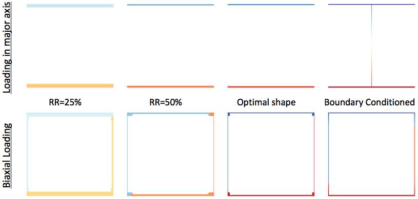
Figure 4.1.1 Optimisation stages and final section with or without set boundary conditions for both biaxial and single axis loading.

4.1.1.1       Top flange

When experiencing bending, the hxb solid cross-section quickly reduces down to material only around the outer perimeter already at RR=25% for both loading scenarios considered. From here, the material thickness narrows down to the even thinner optimal shape. The resulting final thicknesses of the section walls are equal in opposite directions and vary with loading, reducing down to minimal at supports, where there are only shear stresses acting. This can be seen most clearly in the case of cross-section under biaxial bending in the above figure. As the loading in the minor axis is almost half of the loading in the major axis, the vertical walls are also thinner than the horizontal in all levels of optimisation. Therefore, in order to ensure a minimal top flange thickness, a boundary condition needs to be set in order to maintain at least a thickness f for the flat top.

4.1.1.2       Continuity

For the case of loading singly in the major axis, the relative top or bottom of the section will feel most stressed, as it is the furthest away from the neutral axis, therefore material would be required around the outer perimeter to resist these stresses. Shear stresses vary from none at base and top of structure, to maximum value at the neutral axis, which would imply the necessity of a web to connect the flanges as well as to provide shear resistance. However, the stress component from shear has proven to be negligible and no continuity has naturally formed. Therefore a web needs to be introduced in order to achieve connectivity between the top and bottom material. The web is placed centrally on the cross-section in order to minimize torsion and a minimum thickness of w_t needs to be defined in order to avoid failure under local buckling and shear.

In the case of biaxial bending, continuity is organically introduced in the cross-section, however with a web thickness varying with loading condition, why is why a minimal web still needs to be introduced, as explained before. What is more, as seen in Figure 4.2.1, material has accumulated at corners for RR=50% and the optimal section, being smoothed out in the design case with boundary conditions applied. Although structurally beneficial, it can be concluded that the material congestion at corners was a numerical iteration error stemming from relatively low stress levels.

4.1.2     Iteration rate

Maximum tension

Maximum Compression

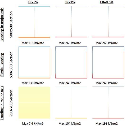
Figure 4.1.2 Converged optimal cross sections for a 500×500 and a 700×700 geometry with varying evolution step sizes

To determine the most efficient dimensional limits and iteration rate to be used, a study is carried out. First, the middle and most stressed cross-section of a 500×500 beam is analysed to the two loading conditions defined in Table 2.3.2.1 to evolution rates 5%, 1% and 0.5%. As seen from the results presented above, ER=5% reaches the lowest level of optimisation with the most material left within its cross-section as well as being the least stressed. The results converge at ER=1%, as with a more refined iteration step of ER=0.5%, the maximum stress and cross-sectional geometry remain unchanged. Therefore it can be concluded that using a 500×500 section with an ER=RR=1% is sufficient for the purpose of this research work.

Proceeding with the 700×700 section, the results never converge, therefore an even smaller iteration step would be necessary. What is more, for the case of ER=5%, the results interestingly present an almost full hxb section as the optimum. This phenomenon occurs as the larger the initial hxb dimensions, the stiffer the section and due to this, the initial principal stresses are well spread, with the maximum being fairly small. Therefore, if the iteration step is too large, the algorithm would want to remove of almost all elements of the mesh, but the flange and web as defined in the boundary conditions. However, in the next iteration the recalculated geometry would result in a significantly smaller area and I-value, leading to a huge jump in principal stresses, at times to values higher than the stress capacity. The program would interpret this as the most optimum solution for the defined ER and revert back to the last iteration. This proves that the larger the initial hxb cross-section chosen for the same loading condition, the more sensitive the results become to the iteration step chosen.

A possible solution to alleviate the issue of removing too much under-stressed material would be to refine the iteration step to a smaller increment. However, this would also bring along an exponential growth in run time of the iteration procedure. Therefore, the most practical approach would be to reduce the initial cross-sectional dimensions to smaller and more appropriate values for the level of stress it is expected to experience. For uniformly loaded steel beams, a span to depth ratio of 18 to 20 is typically used (SteelConstruction, 2017).

4.2    Beam design

A steel beam has been designed for the UDL loading specified in Table 2.3.2.1, to the three methods defined, the first singly with the bone decay analogy, the second with a changing section height and the third with a varying base width. The beam length is analysed by optimising each cut individually and projecting the results to form a whole beam section. As the loading is uniform, the produced design is symmetrical around the middle for all cases, consequently only results for half of the 7m long beam are to be presented in the following tables for clarity. To gain better appreciation of the results, 3D models of full beam designs have been produced in addition to tabulated results. An iteration step sensitivity study for the geometrical and loading condition considered was carried out in the section above, proving that the results are reliable for an ER=RR=1%.

4.2.1     Method 1: Full bone decay analogy

4.2.1.1       Loading in major axis

As predicted, the most optimum cross-section converges into an I-beam shape in the case of loading in the major axis, presented in Figure 4.2.1. The single exception to this rule is the cross-sectional shape at the support, where there are no bending stresses with only shear stresses acting on the section. As can be seen from colour scale presented in the figure below, the stresses in the top flange at the end support are near zero due to the lack of bending stresses. The flat top boundary condition has ensured for the support to maintain a T-beam shape as the bone decay analogy was allowed to only eliminate the under-stressed bottom flange.

Maximum tension

Maximum Compression

At position x (mm):	0	700	1400	2100	2800	3500
Area (mm2):	3480	7952	5968	6960	7952	7952

Figure 4.2.1 Steel beam design for bone decay analogy with RR=1%

Also as expected, the cross-sectional area grows with bending stress, with an exception at position x=700, closest to the support. This is explained as an anomaly stemming from the iteration sensitivity rate. The sensitivity study conducted previously, proved that the results are correct for an ER=RR=1% at the mid-section, however close to the end of the beam, the stress levels decrease to levels too small for the 1% step size to correctly iterate. Therefore, the results are reiterated with RR=0.5% and presented below to prove this hypothesis.

Maximum tension

Maximum Compression

At position x (mm):	0	700	1400	2100	2800	3500
Area (mm2):	3480	4976	5968	6960	7952	7952
Top Plate (mm):	4	6	8	10	12	14
Base Plate (mm):	0	4	6	8	10	12
I value (106 mm4):	93.3	213	286	346	405	405
Total volume (m3):	0.044
Max deflection (mm):	17.9

Figure 4.2.2 Updated beam profile analysed to RR=0.5%

As seen from the above results, with a further refined iteration step the cross-section near the support reaches a much higher level of optimisation, shredding nearly half of its cross-sectional area in comparison to RR=1%. The rest of the beam section has converged to the same geometries with the initial step size, from which it can be deduced that the abnormality was a results of the low level of stress.

The final beam section shows a uniform growth in cross-sectional area, with the flanges growing in thickness linearly when moving towards the mid-span. The web maintains the predefined minimum girth of w_t=4mm, which further proves that the effects of shear stress are negligible and no web thickening is required for the magnitude of stress experienced. As mentioned, the total volume and maximum deflection are achieved by mirroring the resulting cross-sectional geometries about the centre point of the beam, from where the iterated points are extrapolated to meet up as a whole beam. To illustrate this, a solid 3D model is presented below of the resulting beam section calculated from Method 1, together with a line-model where single cross-sections are drawn out.

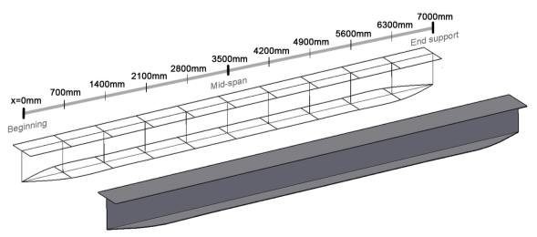
Figure 4.2.3 Resulting beam geometry for Method 1, loading only in major axis

4.2.1.2       Biaxial loading

Maximum tension

Maximum Compression

At position x (mm):	0	700	1400	2100	2800	3500
Area (mm2):	5460	6199	7936	9412	8920	9904

Figure 4.2.4 Bone decay optimisation profile for beam under biaxial loading with RR=1%

The bone decay analogy has been implemented in a beam under bending in both axes with the results presented above. Again it can be noted how near the support the optimisation procedure collapses and some ‘spikes’ of material are formed in the web 700mm along the beam length. As already proved with the case of loading in the major axis, the irregularity in the optimised shape can be explained as a result of using inappropriately large RR for the stress it is experiencing. However, as a further anomaly, at location 2100mm along the beam the converged cross-sectional area experiences a jump and consecutive decreases when moving on to a closer to middle location. It my be hypothesised that this might be a results of a more complex loading nature, which is why the whole beam has therefore been reanalysed for an RR=0.5%. Nevertheless, a definite conclusion can be made that the iteration rate chosen and proved in the earlier study is in fact insufficient for lowest stressed cross-sections, which is why a more refined rejection rate has to be chosen for reliable results.

Maximum tension

Maximum Compression

At position x (mm):	0	700	1400	2100	2800	3500
Area (mm2):	5460	6460	7444	8920	8920	9904
Top Plate (mm):	4	5	7	10	10	12
Base Plate (mm):	0	0	5	8	8	10
I value (106 mm4):	148	214	294	385	385	444
Total volume (m3):	0.055
Max deflection (mm):	19.4

Figure 4.2.5 Bone decay analogy in biaxial loading with RR=0.5%

The results for a RR=0.5% reiteration in Figure 4.2.5 show how a smaller iteration step has smoothed out any anomalies to an even growth in cross-sectional area as the loading increases towards mid-span. The optima depict an open U-section as the most efficient for at least 700mm from the end spans, evolving into a box-section further along the beam. Apart from this, the top and base plate show a steady growth in thickness in response to the developing degree of stress. In addition to bearing shear stresses, in the case of bi-axial loading the web is also carrying any out of plane bending stresses, however the default 4mm thickness has proved to be sufficient through the beam section, with the web maintaining the minimum thickness throughout the whole span.

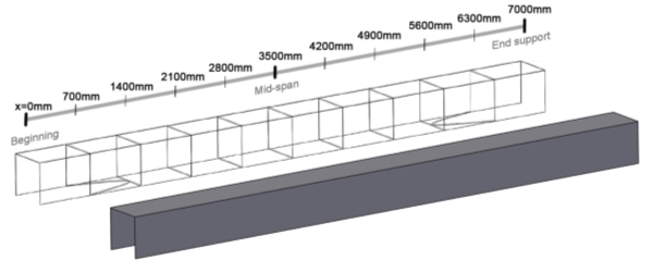
Figure 4.2.6 Steel beam section under bi-axial loading, optimised to the bone decay analogy

4.2.2     Method 2: Changing section height

In chapter 4.1.2 it was predicted for the cross-sectional area and depth of the beam to vary along the length accordingly to the stress it is experiencing. As noted in the previous section when analysing beam to the bone decay analogy, then the cross-sectional area did indeed vary with the magnitude of loading, however the depth of the optimal section remained constant. This is due to how the optimisation procedure has been set up, where maximum bending stresses experienced will always occur at the outer boundaries of the cross-section as the distance to the neutral axis is the largest. As a result, all material will automatically congest around the outer perimeter, keeping the converged section always at the predefined height h.

In order to analyse a scenario where the effects of changing beam depth could be analysed, a second method of optimisation has been defined with a procedure as explained in chapter 3.3.3, where the section is allowed to diminish in height in accordance to the stresses acting at each section.

4.2.2.1       Loading in major axis

Maximum tension

Maximum Compression

At position x (mm):	0	700	1400	2100	2800	3500
Area (mm2):	3980	7096	7388	7644	7840	7904
Height (mm):	256	285	358	422	471	500
I value (106 mm4):	35.7	124	201	284	358	386
Total volume (m3):	0.050
Max deflection (mm):	24.3

Figure 4.2.7 Section with varying height under loading in major axis

As seen from results above, the bottom of the section organically follows a similar curve to the bending moment the beam is experiencing, starting from the full height at mid-span and ranging down to roughly half of the original at support. The flange and web thicknesses are kept constant throughout the span, with the web at 4mm, top flange at 14mm and bottom flange at 12mm as per the middle section from Method 1. An exception to this occurs at the support, where the flanges are experiencing near zero stresses, therefore the bottom one has been deemed as redundant and removed, with top being maintained for constructability reasons. The full beam section has been modelled below, where the changes in section depth are clearly seen.

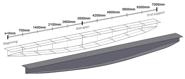
Figure 4.2.8 Method 2 optimised beam line-model and solid 3D model in case of loading in major axis

4.2.2.2       Biaxial loading

Similarly to loading in only major axis, the depth of the beam under loading in both directions varies in response to the level of stresses experienced, as depicted in figure below. The variations in final depths achieved for the box sections are more extreme in comparison to the I-beam section, with the section height decreasing from its full depth at mid-span down to only a third at support. This is due to the two sides enabling the section to carry the same level of stress at a shallower section height.

Maximum tension

Maximum Compression

At position x (mm):	0	700	1400	2100	2800	3500
Area (mm2):	3732	7696	8472	9040	9416	9903
Height (mm):	168	224	321	392	439	500
I value (106 mm4):	76.6	77.7	169	260	333	444
Total volume (m3):	0.058
Max deflection (mm):	27.8

Figure 4.2.9 Box-section with varying depth under bi-axial loading

What is more, near the supports the section opens up to form a U-shape, as without any bending stresses, the bottom plate is no longer required. Other than this exception, the beam profile maintains a constant wall thickness of 4mm, 12mm top and 10mm bottom flange thickness from the original section optimised to Method 1, with the full span modelled below.

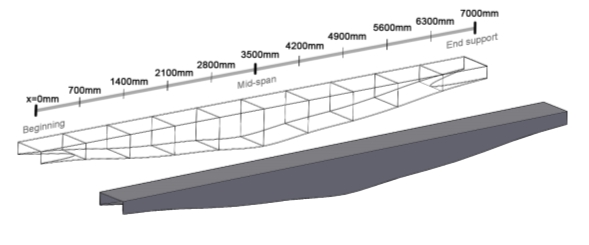
Figure 4.2.10 Box section with a changing height, with optimised beam depicted as solid as well as line-model

4.2.3     Method 3: Changing flange width

Finally a third variation of the bone decay optimisation procedure is developed. As discussed above in chapter 4.2.2, material will start congesting around the outer perimeter of the section. In the case of major loading, material stresses are roughly constant along a slither of material with only slight variations induced by shear stresses. Therefore, the section will naturally spread stresses evenly across the whole breath available, maintaining a constant flange breath throughout.

In order to be able to analyse the effects of a changing flange breath, the third optimisation method was developed as explained in 3.3.4, where the dimensions of the top flange and web are to be kept constant and the breadth of the base is allowed to vary. This analysis was undergone only in the case of loading in the major axis, with the results as outlined above.

Maximum tension

Maximum Compression

At position x (mm):	0	700	1400	2100	2800	3500
Area (mm2):	4310	5636	6656	7304	7724	7864
Base width (mm):	4	114	284	392	462	500
I value (106 mm4):	115	205	310	310	362	405
Total volume (m3):	0.047
Max deflection (mm):	19.8

Figure 4.2.11 Optimal section for loading in major axis with changing flange width

From the results of Method 1 at centre span, the flange and web thicknesses are taken to remain constant throughout the section, with the web at 4mm, top flange at 14mm and bottom flange at 12mm. The width of the base varies non-linearly along the span of the beam, maintaining its original 500mm breadth and reducing to none at supports in response to the actions felt by section, as seen from results presented above. The full geometry of the beam is as presented below.

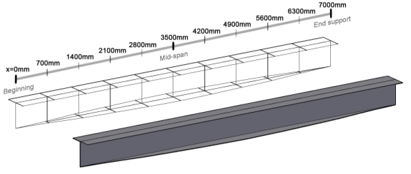
Figure 4.2.12 A line-model and solid 3D model of beam with optimised base flange

4.3    Cross-sectional areas

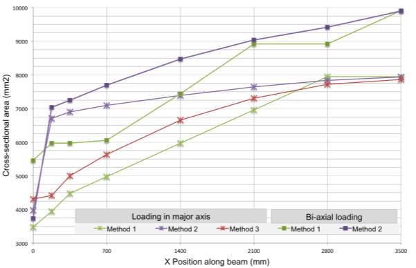
Figure 4.3.1 Optimised cross-sectional areas for each method plotted against major moment experienced

The resulting profile areas for beams under major loading or bi-axial loading optimised to all three methods considered as summarised above. Further to the results presented previously, additional cuts have been optimised nearer to support at 175mm and 350mm from support in order to establish a pattern in optimisation behaviour under low levels of stress.

4.3.1     Loading in major axis summary

From Figure 4.3.1, it can be deduced that the least material throughout the span of the beam is used when optimising to the bone decay analogy as per Method 1. Conversely, at position 2800 near the mid-span, the resulting cross-section was actually the least optimum. Moving towards the support from the aforementioned point, the material needed to maintain the level of stress experiences a steep and steady decline, losing almost 60% of the original cross-sectional area.

With a changing height, the beam optimised according to Method 2 is the least efficient of the three, losing about 16% of its mid-span section size at 175mm away from support. Moving closer to the ends of the beam, shear stresses replace bending stresses as the most critical loading case and the optimal cross-section can shed the weight of its bottom flange, bringing along the steep drop in cross-sectional area.

Method 3, only carried out in the case of loading in major axis, shows a progressively sharpening decrease in cross-sectional material, when moving from mid-span towards the supports, losing approximately 47% of its original section area. An exception to this is the modest kink at x=175mm, by which the whole base flange has been removed and the section is allowed to remove area by reducing its height.

4.3.2     Bi-axial loading summary

In the case of a beam loaded in both axes, the optimisation behaviour to Method 1 is slightly more eccentric than that of loading in purely the major axis. The beam experiences steady drops in cross-sectional size, plateauing near support as well between 2100 o 2800mm from the pinned ends. From most stressed region to least, the section has shed roughly 44% of its weight.

In the case of a varying section height, the rate of losing material when moving along the section is near identical to that of loading in single axes. The drop experienced near support is due to same reasons as stated above, with the bottom flange deemed as redundant and removed. Up to that point, the cross-section at x=175mm was about 29% lighter than the maximum, showing a higher level of optimisation that its counterpart loaded only in the major axis.

4.4    Bending capacities

The elastic moment capacities in the major axis at all spans been calculated and plotted against the bending experienced in Figure 4.3.2. The results presented below show a relatively uniform performance across all loading scenarios and optimisation methods considered. The cross-sections’ capacities never fall below the moment acting on section, further confirming the reliability of the optimisation procedure set up.

The bone decay analogy for both loading in major as well as bi-axial directions shows consistent capacities throughout the length of the beam, decreasing steadily along the span. As discussed above, a beam under bi-axial loading reaches a higher level of optimisation under Method 2, having to compensate with lower moment capacities, however the strength of the section still remaining greater than the moment experienced. Method 3, only implemented on the case of loading in the primary axis, shows relatively smallest ultimate moment capacities, plotted closely following the line of the bending acting on each section.

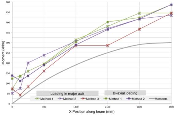
Figure 4.4.1 The elastic moment capacities and moment acting in the major axis are plotted from support to mid-span

The bending capacities in the minor axis have also been analysed and presented below, where the strengths exceed the moment acting on the section by more than 100 kNm on average. As the section has been designed to primarily respond to the major axis component of the combined principal stresses, the exceptional performance in the minor axis is to be expected.

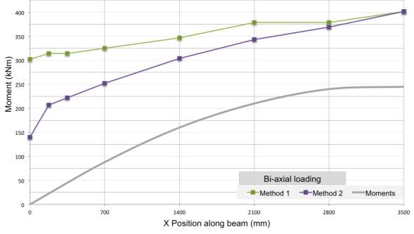
Figure 4.4.2 Bending capacities and moments acting in the minor direction

5         Discussion

The results from all three optimisation methods considered are compared and summarised in the following section. I-sections and box-sections are considered separately in total volume, deflection, constructability and embodied carbon. In addition, a ‘constant’ cross-section has been introduced, where the most middle optimised section has been extruded for the whole span of the beam in order to analyse the effect of tailoring each cross-section of a beam span to the loading it is under, with all results presented below.

To compare the ease of constructability of the methods considered, only currently widely available construction methods such as hot-rolling and welding are considered, excluding the future potential of efficiently producing complex shapes by 3D printing. Therefore, beams with a constant section dimensions have been regarded as design solutions with the highest ease of construction with sections with a varying plate thickness deemed as most complex to achieve.

There are two methods for calculating the embodies carbon within material- Cradle to Gate, which only considers the pure manufacturing process and Cradle to Cradle, which also takes into consideration the afterlife of the material in terms of transport, construction, demolition and recycling. Due to the high potential for recycling of steel, with 99% reused or recycled, the latter method provides much more favourable embodied carbon values. For a conservative estimate, the cradle to gate value for embodied carbon 1.735 kgCO₂e/kg is used. Considering the density of steel as 7800 kg/m³ embodied carbon per unit of volume equals 13 500 kgCO₂e/m³ (TATASteel, 2014).

Table 4.3.2.1 Summary of beam sections developed to different methods

Method	Volume (m3)	Maximum deflection (mm)	Constructability	Embodied carbon (kgCO2e)
I-Beam
Constant	0.056	17.9	Highest	756
1	0.044	19.4	Low	594
2	0.050	24.3	Medium	675
3	0.047	19.8	High	635
Box-Section
Constant	0.069	16.4	Highest	932
1	0.055	19.4	Low	743
2	0.058	27.8	Medium	783

5.1    Volume

As would expect, the most light structure emerges from Method 1, where the bone decay analogy enables the cross-sectional area to grow or decay in size as appropriate to the level of stress experienced. In comparison to the least efficient constant cross-section option, the savings in material volume are at 20.3% to 21.4% for the two loading scenarios.

Method 2, with a varying beam depth gives slightly different results for the two different loading scenarios. In the case of loading in purely the major axis, a reduction in total volume of 10.7% has been reached, while in the case of bi-axial loading this reaches up to 16.0%. With results from section 4.4.2, where moving along the beam’s length the bi-axially loaded beam shed a higher percentage of its maximum cross-section, it can be concluded that optimisation with varying section depth works more efficiently on sections loaded in two directions. The results illustrate potential for considerable savings in material, however as the base flange accounts for relatively more of the cross-sectional mass than the web, than the customisation of the flange thickness itself could leave room further savings.

It is to be noted that with a varying I-beam bottom flange width, Method 3 reaches an extremely high level of optimisation, with a total volume only 2.3% more than that of the bone decay analogy.

5.2    Deflection

The limit considered is span/240 for combined applied load and dead load, which for a 7m beam would deflections under SLS loading as 29.2mm. All solutions are within the stated limit, with Method 2 deflecting most. This was to be expected, as the stiffness of the section is a cubic function of the section height, therefore a shorter section height would lead to a lower second moment of area at each slither, resulting in the highest summative deflection.

With a consistent height and most material, the non-optimised Constant method produces the most stiff sections, followed by Method 2. With a span to deflection ratio of 360, the bone decay analogy has produced two sections with an almost identical stiffness for both loading scenarios.

Again it can be noted how Method 3 performs is only shy off from the extremely similarly to the bone decay analogy, with a maximum deflection at 19.8mm, only 0.4mm shy of Method 1.

5.3    Constructability

Due to the highly varying cross-sectional dimensions resulting from optimisation Method 1, the final beam section is deemed as most complex to construct. In the vase of Method 2 the varying height results in a web of altering height as well as a curved bottom flange. However, as all elements of the section, web and flanges, are of the same thickness, the construction of such a section remains feasible. Similarly with consistent element thicknesses, Method 3 further benefits from a constant element height, leading to a highly achievable section design, with the single complexity being in cutting out the custom bottom flange geometry.

5.4    Embodied Carbon

The total value of embodied carbon is a linear function of the volume of material used, therefore the more optimal a section is, the less carbon is withholds. This is why the most carbon emission are embedded in a constant cross-section, followed by Method 2. The bone decay analogy and Method 3 perform the best, with a notable difference in levels of embedded carbon between I-beams and Box-sections, stemming from the higher cross-section area of the latter.

6         Conclusion

The world steel industry accounts for roughly 5% of the total man-made greenhouse gas emissions, with production quantities on the rise in emerging economies (IISI, 2007). The necessity to design more intelligent and lighter steel structures is further highlighted by the international efforts towards reducing global CO₂ emissions, consolidated with the Kyoto Protocol and the Paris Agreement on Climate Change (UN, 1998, 2015). The current design approach of sizing sections to the maximum stress experienced is inefficient, rendering the majority of the member span to work well below its design capacities. This research work has set out to explore a more efficient distribution of steel in common structural members by defining a bone decay analogy and assessing its application in constructions. Considering three alternative optimisation approaches, more evenly stressed and ultimately more efficient structures are achieved, therefore promising significant savings in material usage and hence embodied carbon.

A design example has been used throughout to establish optimisation behavior for loading in a singular as well as biaxial direction. Alternative starting section geometries were explored and a relation between initial section size and level of stress experienced was established, highlighting the importance of realistic initial dimensions. In the case of the single cross-section analysis, an I-beam section has confirmed to be the closest to optimum shape under major axis loading, with a box-section in the case of bi-axial loading. These fit the standard design sections already used in industry, being the most effective solution in case of simple supports, provided the section was sized correctly. Throughout the examples analysed, the web maintained its predefined minimum girth, proving that the effects of shear stress has been negligible and no web thickening is required for the given loading configurations.

Optimising for the whole 7m span, the final beam sections show a uniform growth in cross-sectional area for all methods considered, with the flanges progressively thickening as moving from support towards mid-span. The full bone decay analogy has proved to be most efficient compared with an equivalent constant section size, with material savings just greater than 20%. A varying section depth demonstrated to be most beneficial for the bi-axial loading configuration, reducing in volume up to 16% in comparison to a constant section sized beam. In the case of loading singly in the major axis, a changing base flange breadth reaches higher material savings of XXX%.

By applying the bone decay analogy, it has been proved that common structural beams could be designed to the same ultimate strength capacity while reducing material weight up to 21%. The methods present considerable savings to be achieved, however the varying web and flange thicknesses are a challenge to manufacture within the scope of technologies readily available nowadays. As 3D-printing technologies are currently unavailable in industrial-scale capacities, a fully bespoke steel profile potential is yet to prove its potential to grow into a new industry standard in the foreseeable future. While these hurdles are still to be overcome, the Method 2 and 3 are highly constructible alternatives that can be manufactured via cutting and welding to varying flange height or breadth. Even with the highly achievable modification of varying bottom flange breadth accordingly to the level of stress experienced, this study has proved that 16% less steel could be used than the current industry norm. This promises fantastic saving that in addition to decreasing embedded carbon, would also reduce the total self-weight of a structure, ultimately scaling down building foundations.

6.1    Future research

6.1.1     Optimised web

The optimisation method developed is based on a cross-sectional approach, where the final beam section is reached via extrapolation along the whole length. Prior to defining a continuity boundary condition, the web was removed by the bone decay analogy as it is experiencing relatively low stresses. As already underlined in chapter 3.3, a constant web spanning the full breadth may not be necessary and further savings in material could be reached when optimising three-dimensionally. The developed beam section can be used as a starting geometry for optimisation in the longitudinal direction, where web would be expected to be removed at mid-span, with negligible shear stresses. An example beam design, optimised in the longitudinal direction in Millipede converges in an arch-like web shape, as illustrated below (Michalatos and Payne, 2012).

Figure 6.1.1 A simply supported beam under UDL optimised on Millipede (Michalatos and Payne, 2012)

6.1.2     Steel structure optimisation

Within the extent of the research project, a uniformly loaded beam with pinned support was considered, however the bone decay analogy has scope to rapidly be expanded to a variety of loading as well as end conditions. The optimisation procedure developed is based around an iterative loop where the geometrical properties and stresses are recalculated with each iteration, however the forces acting along the single beam remain unchanged. Further beam load or support configurations could be mathematically calculated as an extension to the design example developed, although a dull and tedious procedure. As a more attractive alternative, already existing structural design software can be utilised to model the desired end and loading scenario from which the load acting on a beam section can be exported. Structural analysis models are often developed already in the early design phases, with software such as Autodesk Robot Structural Analysis being household names in the construction industry (Autodesk, 2017). By employing existing software the data required for optimisation can potentially be rapidly exported via the use of spread sheets with minimal further resources invested.

Further on, whole steel structures can be optimised elements at a time. In the case of a rigid frame construction, the changes to member stiffnessdess (stemming from changes in member geometry) needs to be accounted for at moment connections, as stiffer members attract more moment. Python’s compatibility with Grasshopper and Rhinocesrours means meameber geometry could be easily be exported and visualised to architectural as well as construction models and drawings (Robert McNeel & Associates, 2017).

6.1.3     Design verification

The calculations on the structural performance of the steel sections are a simplified for the purpose of the report, where possible effects from torsion or buckling are unaccounted for. Due to this, further extensive check and testing of prototypes would need to be performed to conclude the feasibility of the design. Changing dimensions may mean that normal compliance with design codes may checks are not appropriate. In the case of the MX3D pedestrian bridge introduced in chapter 2.3.1.2, the city government of Amsterdam were accomodating for the unconvetional design solution and required a full load-bearing test to prove the acceptability of the design, not the normal procedure (Van der Velden, 2016).

testing would be required to increase the data available and to establish definite rules to height to loading or base width to loading ratios. These could be stanradised to new sets of beam designes to common loading, thereby becoming available even to low budget porjects that would lack the design expertise or budget for optimisation themselves, providing incentive to use less steel even in those types of project. New standard sections- design rules to bottom flange breath to every span etc – these would make saving material affordable in early design phases, when expertiese might be expensive, especially in low budget projects or warehouse design.

References

Adeli, H., 2000. Fuzzy Discrete Multicriteria Cost-Optimization of Steel Structures. Journal of Structural Engineering.

Adeli, H. and Karim, A., 1997. Neural Netwrok Model for Optimization of Cold-Formed Steel Beams. Journal of Structural Engineering, pp. 1535-1543.

Autodesk, 2017. Robot Structural Analysis [Online]. Available from: http://www.autodesk.com/products/robot-structural-analysis/overview [Accessed 11th April 2017].

Burgoyne, C., 2007. Chris Burgoyne – Research Projects. Cambrige University Engineering Department, Structures Group.

Crolla, K. and Williams, N., 2014. Smart Nodes: A System for Variable Structural Frames with 3D Metal-Printed Nodes.

Davidson, S., 2017. Grasshopper 3D [Online]. Available from: http://www.grasshopper3d.com/ [Accessed 26th March 2017].

Eschenauer, H.A. and Olhoff, N., 2001. Topology Optimization of Continuum Structures: A Review. Siegen.

Frost, H.M., 1964. The Laws of Bone Structure. Springfield, IL.

Frost, H.M., 1983. The Determination of Bone Architecture: The minimum Effective Strain. Springfield, IL.

Galjaard, S., Hofman, S., Perry, N. and Ren, S., Optimizing Structural Building Elements in Metal bu Using Additive Manufacturing. In:  Proceedings of the International Association for Shell and Spatial Structures (IASS), 2015 Amsterdam.

GhPython, 2017. Food4Rhino [Online]. Available from: http://www.food4rhino.com/app/ghpython [Accessed 23th of February 2017].

IISI, 2007. The annual  International Iron and Steel Institute  publication World Steel in Figures.

IStructE, 2016. Technical Guidance Note (Level 2, No. 1): Designing a steel beam. The Structural Engineer, 91(1).

Jenkins, W.M., 1991. Towards Structural Optimization via the Genetic Algorithm. Leeds.

Kikuchi, N. and Horimatsu, K., 1994. Practical Shape Optimization for Mechanical Structures. Advances in Design Optimization. London: Chapman and Hall.

Langtangen, H.P., 2011. A Primer on Scientific Programming with Python. Berlin, Germany: Springer.

Meyer Boake, T., 2015. Architecturally Exposed Structural Steel. Basel: Birkhäuser.

Michalatos, P. and Kaijima, S., 2017. Millipede [Online]. Available from: http://www.sawapan.eu/ [Accessed 26th March 2017].

Michalatos, P. and Payne, A., 2012. Printing Material Distributions. Available from: http://liftarchitects.squarespace.com/journal/2012/5/28/printing-material-distributions.html [Accessed 11th of April 2017].

Monolith, 2017. Monolith [Online]. Available from: http://www.monolith.zone/ [Accessed 26 March 2017].

Mueller, C., 2016. 3D Printed Structures: Challenges and Opportunities. Insights, Structure Magazine, pp. 34-55.

MX3D, 2017. MX3D Bridge [Online]. Amsterdam. Available from: http://mx3d.com/ [Accessed 22 March 2017].

Python, 2017. Python.org [Online]. Python Software Foundation. Available from: https://www.python.org/ [Accessed 23th of February 2017].

Querin, O.M., Steven, G.P. and Xie, Y.M., 1998. Evolutionary Structural Optimization (ESO) Using a Biodirectional Algorithm.

Querin, O.M., Steven, G.P. and Xie, Y.M., 2000. Evolutionary structural optimisation using an additive algorithm. Finite Elements in Analysis and Design, 34(3–4), pp. 291-308.

Reiter, T.J., 1996. Functional Adaption of Bone and Application in Optimal Structural Design. Düsseldorf.

Robert McNeel & Associates, 2017. Rhinoceros [Online]. Available from: https://www.rhino3d.com/ [Accessed 11th April 2017].

Rozvany, G.I.N., 2009. A Critical Review of Established Methods of Structural Topology Optimization. Seoul.

Saumarez, R.C., 1986. An analysis of action of intercostal muscles in human upper rib cage. Journal of Applied Physiology, pp. 690-701.

Sigmund, O. and Maute, K., 2013. Topology optimization approaches. Structural and Multidisciplinary Optimization, 48(6), pp. 1031-1055.

SteelConstruction, 2017. Framing Schmatics [Online]. Available from: http://www.steelconstruction.info/Framing_schematics [Accessed 3rd April 2017].

Tam, K.M.M., Coleman, J.R., Fine, N.W. and Mueller, C.T., Stress Line Additive Manufacturing (SLAM) for 2.5-D Shells. In:  Proceedings of the International Association for Shell and Spatial Structures (IASS), 2015 Amsterdam. Future Vision.

TATA, 2016. Modified Forms of Steel Sections [Online]. Available from: http://tatproddel.tat.cloud.opentext.com/sites/constructionuk/default/en/reference/teaching-resources/architectural-teaching-resource/technology/standard-steel-forms/modified-forms-of-steel-sections [Accessed 18th of December 2016].

TATASteel, 2014. Steel Construction – Embodied Carbon. The British Constructional Steelwork Association.

UN, 1998. Kyoto Protocol to the United Nations Framework Convention on Climate Change.

UN, 2015. United Nations’ Paris Agreement.

Van der Velden, G., 2016. MX3D Making Final Preparations for Amsterdam 3D-Printed Bridge. Available from: https://agmetalminer.com/2016/11/29/mx3d-making-final-preparations-for-amsterdam-3d-printed-pedestrian-bridge/ [Accessed 11th April 2017].

Verbart, A., 2015. Topology Optimization with Stress Constraints. TU Delft.

Xie, Y.M. and Steven, G.P., 1997. Basic Evolutionary Structural Optimization. Evolutionary Structural Optimization. London: Springer London, pp. 12-29.

Xie, Y.M. and Steven, H.P., 1992. A Simple Evolutionary Procedure for Structural Optimization. London.

Zhou, M. and Rozvany, G.I.N., 2001. On the Validity of ESO Type Methods in Topology Optimization.