ABSTRACT

With aging, steel pipelines for oil and gas transmission undergo corrosion defects that may compromise the integrity of such structure. This work presented a review on most common type of corrosion in the petroleum industries and methods industrially used for burst pressure evaluation of corroded steel pipelines such as, ASME B31G, DNV RP-F101, and PCORRC. According to several studies, the mentioned methods yield in general conservative results that may lead to unnecessary repair of pipelines. This work also reviewed two new models by Shuai et al. and Zhu that provides more approximated results, however these models do not account for multiple corrosion defects. As such, further investigation for a more accurate burst pressure corrosion assessment model is critically important. Using the nonlinear finite element method in Solidworks, a numerical FE model was developed and used to predict the failure pressure of standard API 5L X65 and X80 Steel pipes containing single external corrosion defect. The proposed model was validated with full-scale pipe burst tests data available in published references. Comparison of the numerical model with experimental and standard methods showed that the model can satisfactorily predict the failure pressure of mid and high grades of steel. The model showed excellent calculation precision, being able to predict the failure pressure within an average of 1.7% to 12% margin of error. However, the model has been only tested for single corrosion defect in isotropic steel pipes.

Table of Contents

ABSTRACT

ACKNOWLEDGEMENTS

CHAPTER 1

INTRODUCTION

1.1. Project overview

1.2. Aims of the project

1.3. Objectives

CHAPTER 2

LITERATURE REVIEW:

SECTION 2.1: CORROSION IN OIL AND GAS PIPELINES

2.1.1. Corrosion in oil and gas pipelines [2]

2.1.2. Corrosion Mechanism in oil and gas pipelines and Prevention

SECTION 2.2: BURST STRENGTH

2.2.1. Burst pressure in oil and gas pipelines

2.2.2. Burst failure criterions

SECTION 2.3: REVIEW OF EXISTING ANALITYCAL MODELS

2.3.1. ASME B31G model [6, 15]

2.3.2. DNV RP-F101 Model [17]

2.3.3. PCORRC Evaluating Method [15, 6]

2.3.4. Shuai et al. evaluation model

2.3.5. Zhu

SECTION 2.4: FINITE ELEMENT MODELS

2.4.1. Material nonlinearity and strain hardening effect on burst pressure

CHAPTER 3

CONCEPT AND DESIGN OF THE NUMERICAL FE MODEL

3.1. Geometry and symmetry

3.2. Assumptions

3.3. Modelling corrosion defect

3.4. Material properties and pipeline profile

3.5. Boundary conditions

3.6. Meshing

3.7. Burst Failure criterion

CHAPTER 4

ANALYSIS OF RESULTS, DISCUSSION AND RECOMMENDATIONS

SECTION 4.1: METHODOLOGY AND CALCULATIONS

4.1.1. Calculation example

4.1.2. Model validation and comparison to standard methods

SECTION 4.2: PARAMETRIC ANALYSIS

4.2.1. Effect of width on failure pressure

4.2.2. Effect of depth on failure pressure:

4.2.3. Short and Long corrosion defect effect on the remaining strength

SECTION 4.3: MODEL LIMITATION AND RECOMMENDATION

CHAPTER 5:

CONCLUSION

REFERENCES:

APPENDICES

Appendix A: SIMULATION DETAILS

Appendix B:  WORK PROGRAMME

Appendix C:  RISK ASSESSMENT

Appendix D:  MATLAB SCRIPT

CHAPTER 1

INTRODUCTION

1.1.     Project overview

Steel pipelines play extremely important roles in the oil and gas industry worldwide. It provides the most efficient, safe and economical mean for large-scale hydrocarbons’ conveyance, from production fields to refineries, processing plants, as well as to deliver oil and gas derivatives to consumers. Transmission pipelines, cross-country, typically transport unrefined crude oil or petroleum products such as gasoline, diesel and jet fuel, refined fuel oils and the already processed natural gas, liquid propane and butane [1, 2, 3].

Oil and gas industries use low strength, mid and high strength steel pipelines depending on the operating conditions. The most commonly used transmission pipelines considered in this work are mid-strength API X65 gas pipelines and high strength API 5L X80.

In general, transmission pipelines are of large diameter with thin wall subjected to high internal pressure. With aging, the pipelines might undergo a very common damage mechanism known as corrosion, that can appear in different shapes and sizes as a result of the internal flow and external environmental conditions. Consequently, the corroded region results in significant loss in the pipeline remaining strength due to significant localized thickness reduction. Subsequently, unexpected failure may occur. Therefore, accurate prediction of burst pressure of corroded pipes is of critical importance.

1.2.     Aims of the project

The aim of this work is to investigate the accuracy and limitations of existing burst failure assessment methods and propose a numerical solution to evaluate the integrity of thin-walled pipelines containing single corrosion defect and to determine whether the pipeline can continue to service, repaired or replaced.

1.3.     Objectives

• Outline pipelines technologies and importance for transportation of hydrocarbons;
• Outline corrosion mechanisms, damage detection and protection;
• Review of existing models for burst strength prediction;
• Design and develop a numerical FE model to evaluate the remaining strength of corroded steel pipes using Solidworks package;
• Investigate burst pressure behaviour in thin-walled X65 and X80 steel pipelines;
• Perform parametric analysis and establish the effect of various geometric and material parameters on burst strength;
• Discuss findings and their application for the design;

CHAPTER 2

LITERATURE REVIEW:

SECTION 2.1: CORROSION IN OIL AND GAS PIPELINES

2.1.1.  Corrosion in oil and gas pipelines [2]

With aging, different corrosion types and sizes may occur in the pipeline leading to unexpected failure.  Steel corrosion in the oil and gas field is mainly non-uniform corrosion that results from an electrochemical process, which involves electrons transfer from iron atoms in the metal to oxygen or hydrogen ions in water.

The most frequent forms of corrosion in petroleum industries’ transmission pipelines are:

• Sweet corrosion: is a CO₂ corrosion type, occurs when dry CO₂ gas is mixed in aqueous solution causing an electrochemical reaction between steel and the aqueous phase.
• Sour corrosion: is an H₂S corrosion type, due to metal contact with hydrogen sulphide and water.
• Galvanic corrosion: Also known as bimetallic corrosion, occurs when two or more dissimilar metallic materials are coupled and exposed to an electrolytic environment, leading the less noble material to corrode.
• Microbiologically induced corrosion: Caused by the bacterial activities resultant from an excess of H₂S, CO₂ and other acidic components in the flowing fluid that corrodes the pipes by toxicity.

Steel pipelines in the oil field can undergo internal or external corrosion or even both at the same time. The fluid carried usually contains hydrogen sulphide (H2S), carbon dioxide (CO2), chlorides from salt water and many other substances from the production of hydrocarbons. The mixture of carbon dioxide or hydrogen sulphide and water or oxygen usually results in a very acidic component that can destroy steel. If the mixture involves salt water, the attack becomes even more aggressive. This leads to greater internal corrosion damage [1,2]. Not only that but also an excess in the fluid velocity, combined with the unknown slurry bacteria can wear out or erode the pipeline internally. Transmission pipelines can be installed above or below the ground depending on the company preference. Irrespective of the chosen installation system, over time it can be under the effects of external corrosion. When the pipe is installed below ground, i.e. buried, and is not properly protected, the material with almost no electrical potential, such as soil, behave as a cathode (negatively charged). Whereas the unprotected pipe behaves like an anode (positively charged), as a consequence metal transference, from pipe to soil, takes place by means of electrons transfer promoted by the water and other medias (electrolyte) contained in the soil. In addition, the connection of dissimilar pipe materials, of different electrode potential, may also lead to serious corrosion damages by the same principles, and this is known as galvanic corrosion. Therewithal, external corrosion can be also due to the pipeline exposure to the harsh environmental condition, such as cold, heat, moisture, chemical pollution, etc.

2.1.2.  Corrosion Mechanism in oil and gas pipelines and Prevention

Corrosion is the most important damaging mechanism in oil and gas pipelines. Generally, it appears at either high-stress concentration points or zones such as seams or welded zone, in the form of general or localized corrosion. According to published researches [1,2], one main reason for pipeline leakage is external corrosion.

Pipelines buried for a very long period, i.e. over 5 years usually experience some sort of corrosion defect, especially cracks. The combination of residual or Hoop stress with the environmental condition of the soil results in crack initiation and crack propagation along the thickness of the pipeline, because of the amount of oxygen and moisture that the soil contains. While the pipeline is operational if corrosion continues, the cracks can grow from small to critical scales, weakening the strength of the material and eventually there will be fluid leakage or worst, sudden pipeline failure known as burst failure [4].

There are several ways to control corrosion in steel pipelines. Amongst the most effective corrosion preventions methods, cathodic protection and coating are the most used. However, coating alone is not sufficient to protect the pipe. The coating is a temporary protection method, used to prevent the pipe during operation. Cathodic protection, on the other hand, prevents it from corroding and reduces deterioration rate [2].

SECTION 2.2: BURST STRENGTH

2.2.1.  Burst pressure in oil and gas pipelines

Burst pressure, also known as burst strength, is the internal pressure the pipeline can withstand before rapture or burst as named. This means that if the internal pressure in the pipe reaches its critical pressure or is further increased the pipe will burst. Oil and gas pipelines carry many hydrocarbons that represent a danger to the environment, and the fluid pumped through the pipeline exerts pressure on it, that if exceeded will cause the pipeline to fail under burst. If the burst then takes place, there will be oil spillage leading to environmental damages that result in the company losing a huge amount of money for cleaning up, or in the worst case scenario affecting animal, plant or even human’s life.

It is well known that corrosion affects adversely the remaining strength of the pipeline. The more corroded the pipeline is, the greater the likelihood of burst under certain pressure condition. With time, corrosion can propagate in the pipeline in several ways, depending on the environmental and operating conditions, and the type of fluid carried.

Richard M. Peekema [5], in the article “Causes of Natural Gas Pipeline Explosive Rupture’’ briefly summarized 5 cases of pipeline explosion accidents due to burst table 1. Peekema reported that the abrupt and catastrophic release of the compressed gas is what caused the explosion in all the mentioned cases.

Table 1: Gas pipeline explosive rapture since 1985 summarized by R.M. Peekema [5]

	Year/Location	Pipeline	Crater size	NTSB Rep
2010 San Bruno, CA		30 in @ 400 psi	72×2×13 ft	PAR-11-01
Caused by		Fracture originating in partially welded seam
2000 Carlsbad, KY		30 in @ 675 psi	113×51×20 ft	PAR-03-01
Caused by		Severe internal corrosion reduced wall thickness
1994 Edison, NJ		36 in @ 1000 psi	140×65×14 ft	PAR-05-01
Caused by		Mechanical damage to external pipe surface
1986 Lancaster, KY		30 in @ 1000 psi	500×30×6 ft	PAR-87-01
Caused by		Failure to detect corrosion caused damage
1985 Beaumont, KY		30 in @ 1000 psi	90×38×12 ft	PAR-87-01
Caused by		Undetected atmospheric corrosion damage

Corrosion of any kind significantly reduces the strength of the material, the capacity of the pipeline to resist failure under pressure. When corrosion gets severe through the pipeline, even under its operational pressure condition the pipe may undergo a damage mechanism, which in general is by burst failure. A corroded pipeline is said to be safe when its operating pressure is below its burst pressure multiplied by the appropriate safety design coefficient [7].  Therefore, accurate prediction of burst pressure in oil and gas transmission pipelines that contain single or colonies of defects are demandingly important. Pipeline integrity assessment is still a challenge in the engineering design world, as up to today there is neither analytical nor numerical model that can accurately predict the residual strength of low, mid and high-grade of steel pipelines with different defect sizes and shapes. So far, the numerical, empirical and even analytical existing prediction models are lacking accuracy and consistency, when compared with experimental results. The range of their application is still limited.

2.2.2.  Burst failure criterions

FEA (Finite Element Analysis) methods are numerical solution methods based on continuous mechanic’s theory that can accurately estimate the stress, strain and displacement/deformation of any structure, be it complex or not, even with corroded regions, provided the analysis is correct. However, conventional FEA methods cannot estimate whether a corroded pipe will fail under a specific load unless a failure criterion is set forth.

In order to improve the estimation of the residual strength on pipelines, there should be a failure criterion, which is able to determine when failure will take place. Over the years, several criterions have been put forward attempting to predict burst failure pressure on steel pipelines. They are summarized in this work as:

1. Average Shear Stress Yield Theory (ASSY):

 ASSY is a new yield theory proposed by Zhu and Leis [7], based on the average equivalent stress of Tresca and Von Mises yield criterions. It assumes that if the average shear stress of the material reaches its critical value, plastic yield will take place. However, this criterion was only developed and tested for defect-free pipelines.

 

2. criterion of elastic limit [8]:

The elastic limit criterion assumes that if the equivalent Von Mises stress at the corroded region exceeds the yield strength of the pipe’s material the pipe is not safe and may risk burst failure. The criterion is of simple complexity, which makes it convenient. However, it is over-conservative since it limits the stress analysis to only the elastic region of the pipe. As result, this criterion leads to the unnecessary replacement of the pipeline that result in unnecessary cost. This criterion is more suitable for elastic failure design.

 

3.  Criterion of plastic limit state [9]

This criterion is based on the plastic limit of the pipe. It assumes that if the maximum Hoop stress in the pipe defect zone reaches the UTS of the pipeline the pipe will experience plastic deformation and fail. This criterion completely ignores the post-yielding effect of the material, hence is a conservative criterion.

 

4. Criterion of plastic failure [10]

In the criterion based on plastic failure, the pipe is said to experience local burst failure when the minimum equivalent stress of the corroded defect ligament in the pipe reaches the final post-yielding stress of the material, the true UTS, of the pipe in the FEA calculation.

For many years, researchers used the failure criterion based on UTS to assess the failure pressure on corroded steel pipes. Souza et al. [11], Fu et al. [12] and many others researchers used this criterion to investigate burst in the most widely used pipeline grade X60, for oil and gas transportation. However, some others like Choi et al. [13] suggested that the results provided by aforementioned failure criterion, overestimated burst of corroded pipelines of the same grade. Instead, the authors proposed that failure would occur if the equivalent Von Mises stress in the FEA calculation reaches 80% of true UTS if defect area is of elliptical shape and 90% if rectangular. The proposed criterion improved the accuracy of prediction, since the new criterion was found to yield more approximated results to the experimental ones when compared to others existing models at the time. Because of it, some researches went further investigating the effect of changing the UTS factor in the Von Mises failure criterion. Changing the factor from 80% to 100% of true UTS, Chiodo and Ruggieri [14] found out that two important factors greatly influence the UTS factor and are the strain hardening of the material and the defect’s geometry. For this reason, new studies were required and Zhu and Leis [7] came up with ASSV (Average Shear Stress Yield) a new yield theory. Even though evaluations showed the criterion can provide accurate burst estimation, the model was not tested for corroded pipes.

Therefore, the current situation demands further investigation of a failure criterion for a more accurate assessment of burst pressure in corroded pipelines. However, this piece of work attempts to continue developing an FE model that can better estimate the residual strength of different size, different grades of steel pipes by employing the failure criterion based on plastic failure.

SECTION 2.3: REVIEW OF EXISTING ANALITYCAL MODELS

Researches for evaluating corroded pipelines are long traced from 1960s and up to today, some analytical models have been put forward. Amongst the proposed methods of evaluation, the most widely known and industrially used are ASME B31G, DNV RP-F101, and PCORRC.

2.3.1.              ASME B31G model [6, 15]

The ASME B31G burst evaluation method was first proposed by AGA. Then ASME in 1984 released another version of the previous model, which subsequently underwent some adjustment with the available test data at the time and updated it in 1991. It went from ASME B31G to ASME B31G-1984 and updated to ASME B31G-1991 version. The changes were because the two first models were very conservative. Even though it was safe, still would lead to unnecessary pipeline repair or replacement.

The ASME B31G-1984 model defined flow stress to be

σflow=1.1SMYSand assumed maximum hoop stress to be equal to the yield stress of the pipeline. Not only that but also that for short and long defects, the metal loss area are 2/3

dLand

dLrespectively. The model is limited to a corrosion depth up to 80% of the thickness of the pipe and do not take into consideration corrosion depth of order smaller than 10%.

The ASME B31G-1984 model is given by:

pburst=2tDσflow1-23.dt1-23.dt.1M,0.8L2Dt≤42tDσflow1-dt1-dt.1M,         0.8L2Dt>4           (1)

If

0.8L2Dt≤4, it is considered short corrosion defect and the model assumes a parabolic shape corrosion area with curved bottom.

If

0.8L2Dt>4, long corrosion defect, the model assumes rectangular corrosion area with uniform bottom.

The simplified Bulging/ Folias factor is defined as:

M=1+0.8L2Dt            (2)

where

Pburstis the failure pressure in MPa; SMYS is the minimum yield strength, MPa; D is the outer diameter of the pipe, mm; t is the nominal wall t thickness of the pipeline, mm; d is the defect’s depth, mm; L is the measured length of the corroded area.

Later in 1991, Kiefner and Vieth [16] proposed a modified version (RSTRENG Method) of the ASME B31G model due to its conservativism. The modified model is given by:

pburst=2tDσflow1-0.85dt1-0.85dt.1M         (3)

The proposed modified model assumes,

1. Flow stress:

   σflow=SMYS+68.95MPa;

   (4)

2. Folias Factor:

   M=0.032L2Dt+3.3,L2Dt>501+2.51L22Dt-0.054L24Dt2,L2Dt≤50           (5)

3. Metal loss area:

   A=0.85dL(6)

where A is the average value of rectangular and parabolic area.

In general, the ASME B31G model is a very conservative method developed to evaluate burst failure pressure in lower grade steel pipelines. The ASME B31G-1984 is too conservative for long corrosion defects, but not for short or deep defects. The modified ASME B31G, on the other hand, is not conservative for long-defect but is conservative for short corrosion defect.

2.3.2.              DNV RP-F101 Model [17]

The DNV RP-F101 Evaluating Method, the result of a joint work of DNV and BG technology, consists of two different safety criterion namely Partial safety factor method and Allow stress method. Partial safety method is based on offshore pipeline system whereas Allow stress bases on allowable standard stress design and takes into consideration the strength design factor. In addition, Partial safety method accounts for material and defect inspection uncertainty that increases the accuracy of its prediction. However, it also means longer and more complex equation. Allow stress method, on the other hand, do not take into consideration these uncertainties, which leads to the prediction of a conservative pressure. However, it is a simple and convenient method, preferred by most operators for assessing the remaining strength of pipelines with single defect subjected to internal pressure alone.

• Partial Safety factors method:

pcorr=γm2tSMTSD-t.1-γd(d/t)*1-γd(d/t)*Q,γd(d/t)*<10  ,γd(d/t)*≥1          (7)

And

Q=1+0.31(LDt)2                 (8)

(d/t)*=(d/t)mes+εdStDdt         (9)

where

pcorris the allowable pressure of the pipe with single corrosion, MPa;

γmis the partial factor of safety;

γdis the partial factor of safety to account for corrosion depth;

εdis the factor of the fractile value of the corrosion depth; StD[d/t] is the standard deviation of d/t; SMTS is the specified minimum tensile strength N/mm², and Q is the length correction factor;

• Allow stress method:

pf=2tUTS(D-t)(1-dt)(1-dtQ)       (10)

psw=Fpf                       (11)

where UTS is the ultimate tensile strength of pipe material in MPa; F is the strength design factor of pipeline and

pswis the allowable operation pressure of the pipe;

The DNV RP-F101 criterion can be used for different grade of steel pipes. However, it is more suitable for assessing large-diameter pipes with high strength, and according to J.E. Abdalla Filho et al. [18] this method is not recommendable for short defects, as it results in non-conservativism. For single corrosion defect assessment, the failure model for DNV is same as for ASME B31G but the Folias factor (M) is replaced with the length correction factor (Q) and the flow stress takes into account the UTS instead of SMYS.

2.3.3.              PCORRC Evaluating Method [15, 6]

PCORRC is a Pipeline Corrosion Criterion, proposed by Stephens et al. in 1999, that aims to assess high-grade steel pipes which contains corrosion defect and experience plastic instability. For simplification, the model only considers the length and depth of the defect, disregarding width of corrosion and strain hardening of the material. This method showed to be less conservative than the previous two methods above. Since it accounts for plastic instability, the model uses ultimate tensile strength instead of yield strength. Xian-Kui Zhu stated that even though the PCORRC assessment method was brought forward to better the previous methods, it may sometimes overestimate the burst pressure on high-grade steel pipelines since it does not take the strain hardening effect of the material into consideration [14].

pb=UTS2tD1-dt1-exp⁡-0.157LRt-d   (12)

Pbis the burst failure pressure in MPa and R is the outer radius of the pipe in mm.

J.E. Abdalla Filhoet al. [18] found out during investigation that these assessment methods are in general all conservative when investigating short defect on the pipeline, all of them predict a failure pressure less than the experimental results.

Apart from the models already mentioned, many recent other models were set forward for burst evaluation of pipelines containing corrosion defects. Amongst them, the author of this work chose two best to further evaluate.

2.3.4.              Shuai et al. evaluation model

In 2008, Shuai et al. [6] proposed an empirical formula to evaluate burst failure pressure as the result of several FEM simulations. Different from PCORRC, this model accounts for defect’s width and makes use of the tensile limit strength criterion of the pipe material. According to the author, this model is less conservative than the previously mentioned ones. The model is able to predict the failure pressure with 0.4% to 13.57% prediction error.

pb=σb2tD1-dt1-(0.10751-wπD26+0.8925exp⁡-0.4103LDt1-dt0.2504  )(13)

where,

σbis the tensile limit of the material in MPa and

wis the defect width in mm.

5.              Zhu model

Recently (2015) Zhu [20] managed to develop a semi-empirically model for burst failure evaluation of line pipes with finite-sized defects:

pb=2+343n+14t0D01-d0t0fL0D0t0σuts         (14)

f

is an unknown function of the length of the defect given by:

fL0D0t0=1-11+0.1385L0D0t0+0.1357L0D0t02                (15)

Therefore, the Von-Mises equivalent stress is expressed as:

σM=3PD04t0-d0fL0/D0t0                  (16)

Pbis the burst pressure for the finite-sized defect,

Pis the internal pressure,

D0is the pipe outer diameter,

t0is the thickness of the pipe,

d0the defect depth and

L0the length of the defect.

This model does not take the width of the defect into consideration, according to the author, the assessment model can accurately estimate burst pressure of corroded pipes but further numerical and experimental investigation for high Strength steel pipes is required.

In general, the existing analytical models obtained either theoretically or empirically from FE models were found to be either conservative or limited to some applications, for instance low grade pipelines, because the analysis are based on low stress, between yield and ultimate tensile strength. So motived, this work deals with both mid and high-strength steel pipelines most used in oil and gas transportation.

SECTION 2.4: FINITE ELEMENT MODELS

In addition to the existing analytical models, there are also several numerical models to evaluate burst failure pressure in steel pipelines. Apropos, most of the analytical models are semi-empirically derived from FEA simulations. FEA model is a numerical assessment method that allows studying the failure behaviour of corrosion defects due to burst pressure. However, the accuracy of the estimation depends on the features of the model. It can get quite complex and time-consuming if real corrosion defect shape is to be taken into consideration.

Therefore, when building an FE model for burst pressure analysis it is important that the model is reduced to a minimum size that can yield the accurate results. This means that the symmetry in the pipe geometry and loading conditions have to be taken into account. In order to, if possible, reduce the running time of the overall simulation and get faster but precise simulation results.

For instance, Zhu and Leis [7] performed 22-detailed FEA calculation for static burst analysis using commercial FEA code ABAQUS. Due to plane strain condition, only one-quarter of the pipeline was modelled. However, the model was only developed for defect-free pipelines. Shuai et al. [6], Zhu [15] and many other investigators developed different numerical models for single corrosion defect pipes that yielded a good approximation to experimental values. Chen et al. [20] on the other hand, developed a model to evaluate interacting corrosion defects. Interacting corrosion defect, however, is out of the scope of this topic.

In general, a good finite element method has to consider the material of the model, element meshing size and type, since the model deals with burst failure it has to account to the nonlinear deformation and have a reasonable failure criterion. According to the results of the FE simulations by J.E. Abdalla Filho et al. [13], the use of shell elements rather than the solid elements is more preferable, because it provides more accurate results, i.e. a better approximation to the experimental values. FEA shells are not only more accurate but also renders less computational cost.

These findings motivated the current work to further investigate and develop a numerical model, simple and convenient, able to accurately estimate burst failure pressure of pipes containing single or multiple non-interacting corrosion defects.

2.4.1.  Material nonlinearity and strain hardening effect on burst pressure

Nonlinearity represents one of the main problems for FE model during burst evaluation of corroded pipes. When loaded the pipeline can undergo different deformation stages before it finally collapses. In general, when an internal pressure is applied, the pipe first deforms elastically (linear deformation) if the applied pressure is not greater than the yield strength of the pipe material. The linear deformation is then followed by elastic-plastic deformation if the applied pressure is between yield and tensile strength the pipe. If the internal pressure is further increased, the corroded pipe will undergo necking (in most cases) and subsequently burst. From plastic deformation to final rupture, the deformation is no longer linear.

Burst failure is highly influenced by material’s nonlinear hardening effect, principally for thin-walled pipelines. Recent researches on this area show that different grades of material have a different effect on the behaviour of the failure. Zhu [15] conducted a recent investigation on burst failure criterion of corroded steel pipes in 2015, the criterion is based on previous work done by Zhu and Leis [7] and considered the strain hardening effect on the burst failure pressure. It is given by:

σM=βnσutstrue        (17)

Where

σMis the Von Mises equivalent stress given in FEA,

βnis a correction factor quantified as a function of the strain hardening exponent of the material and

σutstrueis the material true ultimate tensile strength.

For large deformation, the

βnfactor is defined as:

βn=0.933-1.354n+1.45n2      (18)

For small deformation analysis as:

βn=0.933-0.576n+0.164n2      (19)

According to Zhu [15], the expressions given in equations 18 and 19 are only valid for defect-free line pipes. For corroded line pipes, the author defined

βn=0.89for the FEA calculation.

 

CHAPTER 3

CONCEPT AND DESIGN OF THE NUMERICAL FE MODEL

3.1.     Geometry and symmetry

The geometry and dimensions of the pipelines are given in section 3.4. Due to symmetry conditions of load, pipeline geometry and defect of the models could be simplified to significantly reduce complexity and computational time during analysis using static-nonlinear FE method.

Take the pipeline in figure 1, for instance, the geometry and the load applied are symmetric to all possible diametrical planes. The defect is symmetrical to the plane perpendicular to the longitudinal axis at halfway along the length of the pipe and to the plane perpendicular to the vertical axis at halfway along the height of the pipe. Therefore, only one-fourth (1/4th) of the pipe, figure 2, is required to be simulated in order to study how the pipeline will respond under the applied load condition, making use of appropriate boundary conditions.

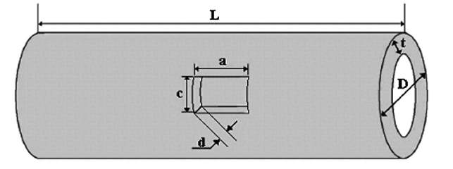
Figure 1: Geometric profile of the pipes tested by Choi et al. [18].

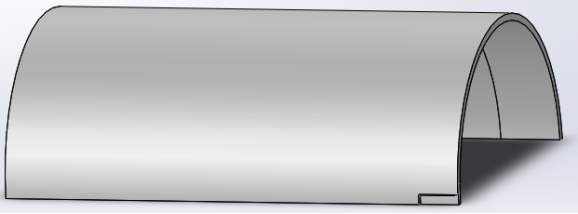Figure 2: Pipe configuration after symmetry condition is applied.

 

3.2.     Assumptions

• Material is isotropic (have properties that are identical in all direction, there is conservation of volume);
• Material experience elastic-plastic deformation, (there will be unrecoverable deformation);
• No influence of the material plastic anisotropy;
• Plasticity Von Mises Model

3.3.     Modelling corrosion defect

Corrosion defect is in simple terms a localized pipe wall reduction. Corrosion assessment methods and defect parameters estimation are available in [23].

Figure 3 presents different finite element models for the corrosion defect. For simplicity, in this study the corrosion defect shape is taken to be as that of a long defect with uniform thickness, as in figure 3d. It is approached by making an extruded cut in the modelled pipe and then apply fillet.

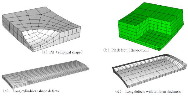Figure 3: Possible finite element models of the corrosion defect in the steel pipe taken from [6].

3.4.     Material properties and pipeline profile

Figure 1 is a geometric representation of an oil and gas transmission pipeline containing single external corrosion defect. The pipeline is 2.3 m long, 17.5 mm thick with 762 mm outer diameter, made of Standard API 5L X65 steel, with the following properties: Young’s modulus of

E=203.5 GPa,UTS

σuts=576 MPa, Yield Strength

σys=467MPaand Poisson’s ratio

ν=0.3. Defect geometry is given in table 1. The stress-strain curve data, figure 4, was implemented into Solidworks to account for large strain deformation in FEA calculation.

 

 

 

 

 

 

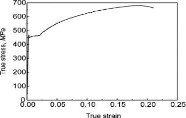
Figure 4: True stress-strain curve data of API 5L X65 from tensile test at room temperature by Choi et al. [13]

Another pipeline made of API 5L X80 Steel (figure 5), higher strength, with the following properties: Young’s modulus of

E=207 GPa,UTS

σuts=740 MPa, Yield Strength

σys=680 MPaand Poisson’s ratio

ν=0.3. Stress-strain curve is given in figure 4 and with defect geometry summarized in table 1 was also tested. The pipeline is of 1912 mm outside diameter and nominal thicknesses 19.89 mm and 13.79 mm.

 

 

 

 

 

 

 

 

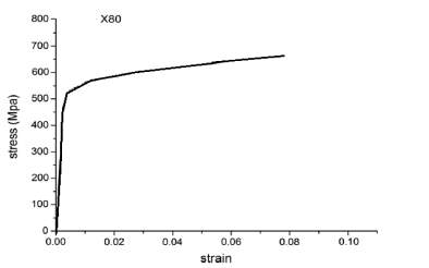
Figure 5: True stress-strain curve data of API 5L X80, from [22].

Table 1: Geometry parameters of pipelines and defects to be tested.

Material	Geometry of pipes		Geometry of defect			Pipe configuration
	D (mm)	t (mm)	a (mm)	c (mm)	d (mm)
X65	762	17.5	200	50	4.4
					8.8
					13.1
			100		8.8
			300		8.8
			200	100	8.8
				200	8.8
				50	4.4
X80	1912	19.89	605.72	50	15.41	HS1
					7.44
			607.74		1.77
		13.79	588.37		10.78	HS2
			589.4		5.45
			586.42		1.54

Where D and t are respectively the outer diameter and nominal thickness of the pipelines and a, c and d the corresponding length, width and depth of the defect.

3.5.     Boundary conditions

In order to accurately predict how the pipeline will fail, where and at what pressure, it is crucial that the pipeline be first constrained, and the constraints have to be as close to the reality as possible.

The constraint is such that no displacement is allowed normal to any of the symmetry planes. The standard boundary condition consistent with this constraint is fixed geometry fixture. This model takes advantage of reference geometry fixture, can be found under advanced fixture, to apply more specific constraints to each of the selected planes. However, Solidworks software provides symmetry boundary condition under advanced fixtures that could be alternatively used and allows previewing the deformation of the whole pipe even though only one-fourth is to be analysed. The applied fixtures in this model are as follow (figure 6):

• Fixed edges on one end of the pipe;
• No displacement allowed normal to the xy and xz plane at the pipe end containing the defect;
• No displacement allowed parallel to z direction of xz plane i.e. z=0;

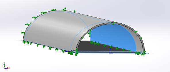Figure 6: Applied boundary condition as described in section 3.5

 

3.6.     Meshing

Meshing is a discrete representation of the geometry of the problem to be studied. Good result’s accuracy comes from appropriate element meshing. If the mesh is very rough, the analysis will not be able to express the stress and location of burst in the pipe. If the mesh is very fine, the analysis will yield more results that are accurate but the process will be time-consuming and will result in unnecessary computational costs.

The aim is to simplify the model as to provide accurate prediction and take less running time. This simplification includes:

1. Modelling only an approximated shape of the defect. The corrosion defect generally is of very complex shape, so for this purpose, there is no need for a very detailed defect shape. Instead, use an approximated shape [6]. For this model use shape d) in section 3.3.
2. Combine or discretize coarse and fine mesh sections. Since the analysis is more focused on the defect region or points, location where likely failure will occur, a considerably coarse mesh is used away from the defect, whereas the defect location will have a finer mesh, as in figure 7. By doing so and implementing appropriate meshing element, the running time is reduced yet the analysis can yield accurate results [6].

These simplifications however, will affect the overall result of the analysis, so it is necessary to introduce a new factor to account for the simplifications made. To avoid the effect of the simplification on burst pressure, stress concentration factor should be considered.

For the purpose of this study, the model used the curvature based mesh with the following parameters (figure 7):

Main body:

• Element size:  Min 25 mm and Max: 125 mm
• Minimum number of elements in the circle: 36
• Element size growth ratio: 1.5
• Draft quality mesh

Defect region:

• Minimum element size: 8.31 mm

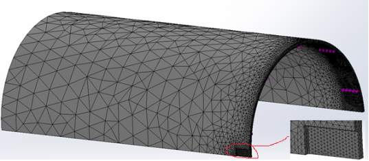Figure 7: Meshing quality plot of the overall pipe (left) and the defect zone (right)

3.7.     Burst Failure criterion

Burst pressure is the ultimate load or failure pressure at collapse. For the purpose of this work, this model assumes the criterion based on plastic failure (Von Mises plastic failure on Solidworks). Burst will occur when:

• The minimum equivalent Von-Mises stress at the defect region equals the UTS of the pipe material;
• For small pit defects when minimum equivalent Von-Mises stress at defect reaches 90% of UTS;

The plasticity Von Mises model in Solidworks package assumes small strain plasticity when small displacement or large displacement is used. It allows the input of the true stress-strain curve (figure 4 and 5) to account for plasticity. For this type of model, the use of the NR (Newton-Raphson) iterative method is recommended. Newton-Raphson is an iteration technique, based on simple idea of linear approximation, to solve equations numerically [24].

CHAPTER 4

ANALYSIS OF RESULTS, DISCUSSION AND RECOMMENDATIONS

SECTION 4.1: METHODOLOGY AND CALCULATIONS

4.1.1.  Calculation example

The suggested FEA model containing external corrosion defect was designed in Solidworks 2015 package. The simulation was conducted for static- nonlinear analysis. Then fixture (boundary conditions), material properties and meshing sizes aforementioned in chapter 3 are applied to the model. Take the case of API 5L X65 with a=200 mm, d=8.8 mm, and c=200 mm corrosion parameters.

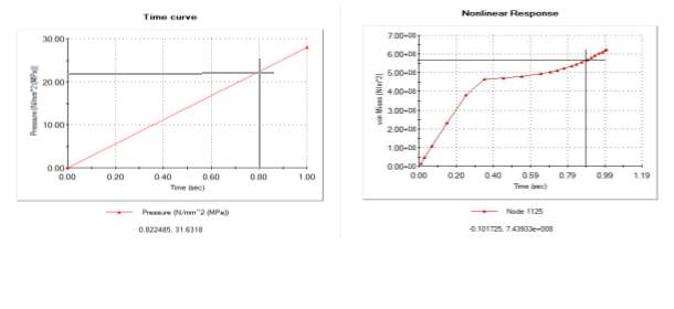For the analysis, a time incremental pressure load (figure 1) was used in the static – nonlinear method in SolidWorks. The nonlinear response (figure 2) of the pipe showed that when the Min. Von Mises stress at the defect ligament reached the UTS of the API 5L X65 Steel pipe, the correspondent applied internal pressure was 22.25 MPa.

 

 

 

 

 

Therefore, 22.25 MPa is the burst failure pressure estimated by this developed FE model. However, the burst experiment conducted by Choi et al. [13] for this same pipe and defect parameters yielded

Pb=22.64 MPa.

The predicted FEA value is an excellent approximation of the experimental value with only 1.73 % estimation error.

The results of the simulation show that, as the expected, the maximum stress concentration on the pipe will be near the defect.  Similarly, maximum strain and displacement take place also in the same region of the pipe since there is reduced material.

Note: See Appendix A, for further details of the simulation results.

 

4.1.2.  Model validation and comparison to standard methods

In order to investigate and validate the range of application and reliability of the purposed model, the model is compared with several experimental data available from published references.

The project considered two distinct grades of steel, most used in oil gas industry operations, to validate the model. Standard burst failure pressure assessment methods such as RSTRENG, DNV and PCORRC are also used to predict the failure pressure given the collected experimental test data. The obtained results are then expressed in tables 1 and 2.

The steel pipeline contained in figure 3 and table 1 represents the grade X65, which is a mid-strength steel grade used for gas transportation, whereas, figure 4 and table 2 represent the results of a high-strength of steel grade X80. The results as shown in figure 3 and 4, tables 1 and 2 indicate that in general all the models including the proposed FE model are acceptably conservative and can accurately predict at what pressure the pipe is expected to fail for both mid and high strength grade of steel. However, the RSTRENG method showed to be too conservative compared to the other three models and can sometimes lead to unnecessary repair or replacement of the pipelines. Amongst all the methods, the proposed FEA model yields the closest results to the experimental ones in table 1, this is a very good assessment method for mid-strength grades of steel. On the other hand, DNV failure pressure method predicts most accurately the values for X80 high strength pipes. However, PCORRC and the FE model predictions are just as close to the experimental results.

Figure 5 shows the comparison of the failure pressure between experimental and the result yielded in FE simulation for both X65 and X80 grade of steel. The results indicate that the model is valid for both grades. The model is able to predict the failure pressure within 1.72% to 11% margin of error for mid-strength X65 and 3.25% to 31.54% for high strength X80 steel pipe. However, in general, the model predicted closest results to the experimental on API 5L X80 grade, the high-strength steel.

Table 1: Experimental and computed burst failure pressure for mid- strength, X65.

API 5L X65 STEEL					3 mm fillet
Length	Width	Depth	P_exp	FEA	RSTRENG	DNV		PCORRC
200	50	4.4 (25%)	24.11	1.03	0.91	1.03		1.00
200	50	8.8(50%)	21.76	0.96	0.86	0.97		0.96
200	50	13.1 (75%)	17.15	0.90	0.83	0.86		0.92
100	50	8.8(50%)	24.3	0.89	0.89	1.01		0.96
300	50	8.8(50%)	19.8	0.97	0.87	0.95		0.96
200	100	8.8(50%)	23.42	0.93	0.80	0.90		0.89
200	200	8.8(50%)	22.64	0.98	0.83	0.93		0.92

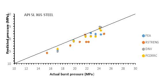Figure 3: Comparison between experiment, FE model and standard methods for X65 steel.

Table 2: Experimental and computed burst failure pressure for high- strength, X80.

	API 5L X80 STEEL						3 mm fillet
Length		Config	Width	Depth	P_exp	FEA	RSTRENG	DNV	PCORRC
605.72		HS1	50	15.41	9.3	1.05	0.89	0.87	0.90
605.72				7.44	17.7	0.93	0.83	1.02	1.02
607.74				1.77	23.3	1.05	0.78	0.99	0.98
588.37		HS2		10.78	5.2	1.32	1.07	1.00	0.99
589.4				5.45	12	0.97	0.82	1.00	0.99
586.42				1.54	16.1	1.08	0.78	0.97	0.96

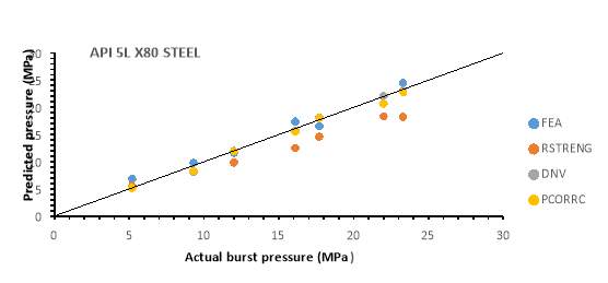
Figure 4: Comparison between experiment, FE model and standard methods for X80 steel.

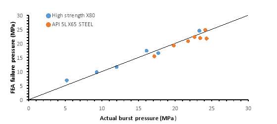
Figure 5: Comparison between experiment and FE model for X65 and X80 grades.

It is important to mention that the stress-strain curve data used for burst estimation for both mid and high strength steel used in the nonlinear method, during simulation, are nothing but a rough estimation of the published graphs. This might have influenced the overall result of the simulations.

SECTION 4.2: PARAMETRIC ANALYSIS

Corrosion defect is a function of three independent parameters namely width, depth and length. In general, it is known that extending defect region means more reduction in the wall thickness the pipe, consequently lower remaining strength. However, this section of the project investigates and discuss the individual effect of each parameter on the burst failure pressure of mid-strength X65 pipe.

4.2.1.  Effect of width on failure pressure

The effect of the width is investigated at constant defect length for two different depths and by changing the ratio of the width to pipeline arc–length as shown in table 3. The ratio ranges from 10 % to 80% of the circumferential length of the pipeline. Figure 6 shows that the width of the defect does not affect much the failure pressure, such that for the worst case scenario varying from 10% to 80% the strength is reduced from 16.54 MPa to 15.98 MPa which accounts only for 5.8% reduction. All the standard analytical methods to evaluate burst failure pressure ignore the effect of the width, table 3 and figure 6 show why even so they can accurately estimate the failure pressure. It is because it has negligible contribution to failure pressure compared to depth and length.

Table 3: Effect of corrosion width to failure pressure.

X65 STEEL	cπD	a= 300 mm d=8.8 Mm		a= 300 mm d=13.1
Width		FEA	ratio	FEA	ratio
231.2	10	22.3	1	16.54	1.00
578	25	22.1	0.99	16.52	1.00
1156	50	22	0.99	16.4	0.99
1618.4	70	21.85	0.98	16.33	0.99
1849.6	80	21.85	0.98	15.98	0.97

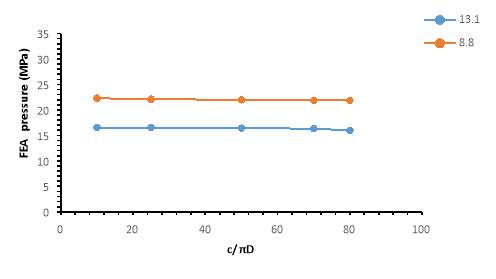
Figure 6: X65 – Pressure change with defect width

4.2.2.  Effect of depth on failure pressure:

Changing the depth of the corrosion adversely affects the remaining strength of the pipeline. For this study, the depth to thickness ratio was changed from 10% to 90%. The ratio represents how deep the corrosion goes into the thickness of the pipe. The change is investigated at a constant width of 50 mm for two distinct defect lengths as shown in table 4. The result in figure 7 shows that increasing the depth of the defect at a constant length the maximum allowable pressure in the pipe decreases in a linear fashion and at a very high slope. Such that a 15% increase in d/t results in about 15.5% reduction in the pipeline remaining strength.

 

Table 4: Effect of defect depth on the failure pressure.

X65 STEEL	dt	a= 300 mm c=50 mm		a= 600 mm c=50 mm
Depth		FEA	ratio	FEA	ratio
1.75	10	28.5	1.00	27	1.00
4.4	25	24.2	0.85	22.5	0.83
6.125	35	22.3	0.78	18.8	0.70
8.8	50	19.25	0.68	16.66	0.62
13.1	75	13.54	0.48	12	0.44
14	80	12.38	0.43	11.45	0.42
15.75	90	9.25	0.32	8.65	0.32

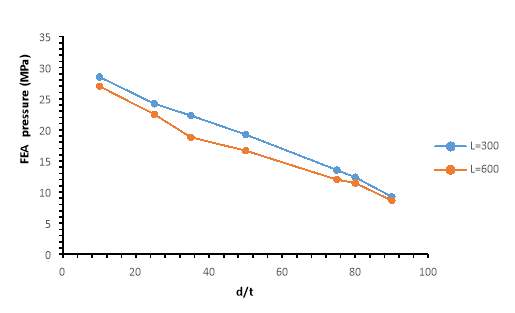
Figure 7: X65 – Pressure change with defect depth.

4.2.3.  Short and Long corrosion defect effect on the remaining strength

In order to evaluate how pressure change for short and long corrosion defect, the API 5L X65 pipe was used again, but this time the thickness of the pipe was adjusted to 13 mm to accommodate the definition of short and long corrosion given by the standard assessment methods.

Corrosion defects are defined as follow:

• If

  0.8L2Dt≤4, short corrosion defect;

• If

  0.8L2Dt>4, long corrosion defect;

Table 5 presents the pipe parameters investigated for long and short corrosion. The 13 mm thickness pipe is kept at constant defect width of 238.39 mm and tested for depths of 30% and 70% of the thickness. The result, as shown in figure 8, indicates that increasing the

a2Dt  reduces the maximum allowable pressure of the pipe in overall. However, it is clear that pressure decay rate is faster when

a2Dt<20(short corrosion defect), whereas when the length of the defect surpasses the outer diameter of the pipe

a2Dt>20(long defect) the change in pressure is very small. The overall trend of the pressure change with

a2Dtis similar to that of a power law decay function.

 

	cπD	Dt	a2Dt	FEA		Corrosion type
	0.1	58.61		dt=0.3	dt=0.7	Short
			2	19.44	13.15
			3.5	18.78	11.46
			5	18.35	10.5
			10	17.51	8.99
			20	16.87	7.94	Long
			35	16.44	7.45
			50	16.22	7.07
			100	15.89	5.96

Table 5: Effect of short and long corrosion defect on X65 Steel

 

 

 

 

 

 

 

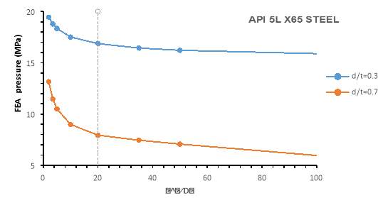
Figure 8: Pressure change with increasing corrosion length.

So far the parameters are looked at as changing independently, however real corrosion defect will hardly experience unidimensional change. It will usually experience a change in either two or even the three parameters. Since the width of the defect does not affect much the failure pressure, we look at changing defect depth and length at the same time. Again figure 8, indicates that the decay rate for short corrosion defect becomes even faster for deeper defects. For instance, for the X65 grade at depth ratio of 0.3 the pressure experience about 13% decrease from 2% to 20%

a2Dt, whereas at 0.7 the pressure decrease is about 40 %.

SECTION 4.3: MODEL LIMITATION AND RECOMMENDATION

The FEM model proposed in this work is restricted to evaluation of simple cases of corrosion such as: in isotropic mid and high strength pipes containing single external or internal corrosion. However real life corrosion cases can get far more complex than this. It may be considered the case when the material is anisotropic, or when there are multiple corrosion and interacting defects along the length or circumference of the pipe.

The model was not used to investigate the failure pressure behaviour in the cases mentioned above. Therefore, further simulation and analysis are recommendable to be conducted to verify the reliability and prediction precision of the model in such circumstances. With further correction, the model could be used to derive a semi-empirical analytical formula to estimate the remaining strength of oil and gas pipelines.

CHAPTER 5:

CONCLUSION

This piece of work investigated the accuracy of existing standard methods to assess the integrity of isotropic steel pipelines, used for oil and gas transportation, containing single external or internal corrosion defect. It was found that most of the existing models aforementioned in this piece of work are conservative methods and with limited application for burst evaluation of corroded pipelines. Amongst all the standards analytical methods, PCORRC stands out for great accuracy to predict failure on both mid and high strength pipes.

A FEM model, based on plastic Von –Mises failure criterion, was developed to evaluate the burst failure pressure of mid and high strength steel pipelines containing short and long-wall thickness reduction defect.

After several simulations, it was concluded that the developed finite element method can be used to effectively investigate and predict the failure behaviour of mid and high strength steel pipelines, containing single corrosion defect. The criterion based on plastic failure can provide good anticipation of the expected results, allowing engineers to decide whether the pipelines are to be repaired or replaced as required.

The model allowed observing that the width of the defect has almost no effect on the failure pressure. However, length and depth adversely affect the remaining strength of the pipe. According to the model, if the depth of the defect exceeds 80% of the thickness, the pipe should be replaced.

Even though the numerical model developed can yield excellent results for burst failure pressure, more grade X40 and X60 steel (low-grade) tests are required to complement the model. The model was not tested either for multiple and interacting corrosion defects. Finally, it is important to review, continuously, existing assessment methods for more precise burst pressure estimation.

REFERENCES:

[1] Tahcker, B.H., Light, G.M., Dante, J.F., Trillo, E., Song, F., Popelar, C.F., Coulter, K.E. and Page, R.A. (2010). Corrosion Control In Oil And Gas Pipelines. Pipeline & Gas Journal, 237(3), pp. 62-66.

[2] Cicek, V. (2013). Cathodic Protection: Industrial Solutions for Protecting Against Corrosion. Wiley, pp.231- 246.

[3] Revie, R. Winston. Oil and Gas Pipelines: Integrity and Safety Handbook, John Wiley & Sons, Incorporated, (2015). ProQuest Ebook Central, pp. 99

[4] Sadeghi Meresht, E., Shahrabi Farahani, T., and Neshati, J. (2011). Failure Analysis of Stress Corrosion Cracking Occurred in a Gas Transmission Steel Pipeline, Eng. Failure Anal., 18, pp. 963–970.

[5] Peekema, R. (2013). Causes of Natural Gas Pipeline Explosive Ruptures. Journal of Pipeline Systems Engineering and Practice, 4(1), pp.74-80.

[6] Shuai J, Zhang C, Chen F, He R. (2008). Prediction of Failure Pressure of Corroded Pipelines Based on Finite Element Analysis. ASME. International Pipeline Conference, 2008 7th International Pipeline Conference, Volume (2), pp. 375-381

[7] Zhu, X. and Leis, B. (2007). Theoretical and Numerical Predictions of Burst Pressure of Pipelines. Journal of Pressure Vessel Technology, 129(4), pp.644-652.

[8] Wang Yung-Shih. (1991). An elastic limit criterion for the remaining strength of corroded pipe. ASME OMAE 10th Int. Conf. off. Mech. Arctic Engrg, Stavanger, Norway, 5, pp:179-186.

[9] Hopkins P, Jones D G. (1992). A study of the behaviour of long and complex-shape corroded in transmission pipelines. ASME OMAE, 11th Int. Con. Off. Mech. Arctic Engrg. Calgary, Canada, 5, pp:211-217.

[10] Fu Bin. (1996). Advanced methods for integrity assessment on corroded pipelines. Proceedings of the 1996 Pipeline Reliability Conference, Houston, USA, pp:1-11.

[11] Souza, R.D., Benjamin, A.C., Freire, J.L.F., Vieira, R.D., Diniz, J.L.C. (2004). Burst tests on pipeline containing long real corrosion defects. Proceedings of International Pipeline Conference, October 4-8, 2004, Calgary, Alberta

[12] Fu, B. and Kirkwood, M.G. (1995). Determination of Failure Pressure of Corroded Linepipes Using the Nonlinear Finite Element Method. Proceedings of the 2nd International Pipeline Technology Conference, Vol. II, pp. 1-9.

[13] Choi J.B., Goo B.K., Kim J.C., Kim Y.J. and Kim W.S. (2003). Development of Limit Load Solutions for Corroded Gas Pipelines. International Journal of Pressure Vessels and Piping, Vol. 80, pp. 121-128.

[14] Chiodo, M.S.G. and Ruggieri, C. (2009). Burst Pressure Predictions of Corroded Pipelines with Long Defects: Failure Criteria And Validation, Proceedings of 2009 ASME Pressure Vessels and Piping Division Conference, Prague, Czech.

[15] Zhu X. (2015) ‘A New Material Failure Criterion for Numerical Simulation of Burst Pressure of Corrosion Defects in Pipelines’, ASME. ASME Pressure Vessels and Piping Conference, Vol. 6(B)

[16] Kiefner, J.F. and Vieth, P.H. (1989). A Modified Criterion for Evaluating the Remaining Strength of Corroded Pipe, Final report on Project PR 3-805 to the Pipeline Research Committee of the American Gas Association.

[17] DNV. DNV RP-F101. 1999, Recommended practice RP-F101 Corroded Pipelines[S].

[18] Abdalla Filho, J., Machado, R., Bertin, R. and Valentini, M. (2014). On the failure pressure of pipelines containing wall reduction and isolated pit corrosion defects. Computers & Structures, 132, pp.22-33.

[19] Besel, M., Zimmermann, S., Kalwa, C., Kippe, T., and Liessem, A. (2010). Corrosion Assessment Method Validation for High-Grade Lin Pipe. Proceedings of the 8 th International Pipeline Conference, Calgary, Canada

[20] Chen, Y., Zhang, H., Zhang, J., Liu, X., Li, X. and Zhou, J. (2015). Failure assessment of X80 pipeline with interacting corrosion defects. Engineering Failure Analysis, 47, pp.67-76.

[21] Lam, P. S., Morgan, M. J., Imrich, K. J., and Chapman, G. K. (2006). Predicting Tritium and Decay Helium Effects on Burst Properties of Pressure Vessels. Proceedings of the ASME Pressure Vessel Piping Conference, Vancouver, BC, Canada, July 23–27

[22] Ma, B., Shuai, J., Wang, J. and Han, K. (2011). Analysis on the Latest Assessment Criteria of ASME B31G-2009 for the Remaining Strength of Corroded Pipelines. Journal of Failure Analysis and Prevention, 11(6), pp.666-671.

[23] Proceedings.asmedigitalcollection.asme.org. (2018). [online] Available at: http://proceedings.asmedigitalcollection.asme.org/data/Conferences/ASMEP/89945/309_1.pdf [Accessed 18 Mar. 2018].

[24] He, J. (2004). A modified Newton-Raphson method. Communications in Numerical Methods in Engineering, 20(10), pp.801-805.

APPENDICES

Appendix A: SIMULATION DETAILS

 Further detail of thestatic–nonlinear response of API 5L X65 Steel pipe subjected to internal pressure, SolidWorks.

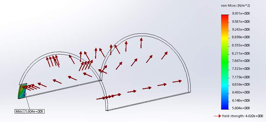
Figure A1: stress distribution on the corroded region of the pipe

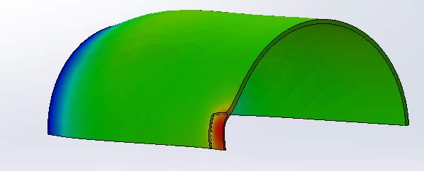
Figure A2: Deformed shape of the corroded pipe with

107displacement deformation scale.

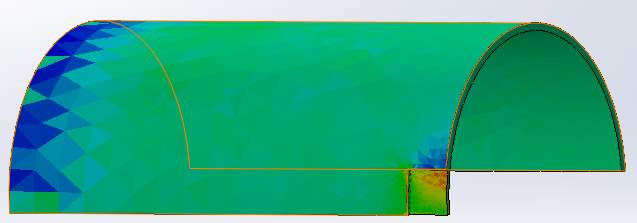
Figure A3: Strain distribution plot

Appendix B:  WORK PROGRAMME

Work Programme: Gant chart and table of activities performed during spring term.

Table 2: Breakdown of activities during spring.
Activities	Start Date	Days to complete	Task
Model improvement Re-meshing, reduce ruing time, etc.	22-jan	14	Task A
Short corrosion defect: FE simulation	05-feb	14	Task B
Short defect analysis and discussion	11-feb	7	Task C
Long corrosion defect simulation	19-feb	14	Task D
Long defect analysis and discussion	25-feb	7	Task E
Parametric analysis	05-mar	7	Task F
Model’s validation and Further analysis	12-mar	14	Task G
Final thesis writing and Poster	19-mar	28	Task H

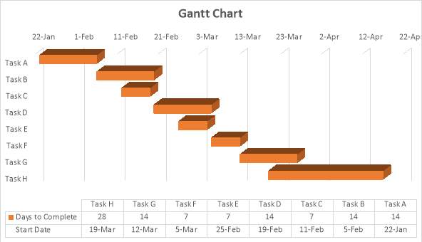
Graph 1: Gantt chart of the work performed during spring.

Appendix C:  RISK ASSESSMENT

Project name:	Predicting Burst Strength of Corroded Steel Pipes
Location of work:	University of Aberdeen (Campus)
Principal Investigator/Supervisor:	Maria Kashtalyan	Signed:	Date:
Assessment Prepared by:	Edmundo Cambolo	Signed:	Date:
Outline description of the work:	Investigating the remaining strength of oil and gas steel pipelines containing a single corrosion defect. Develop a numerical FE model to predict the pressure failure behaviour on the pipeline.
Names of persons carrying out the work:	Edmundo Cambolo

What are the hazards?	Who might be harmed and how?	What are you already doing?	Do you need to do anything else to manage this risk?	Action by whom?	Action by when?	Done
Saying too long in front of the computer	Edmundo. It may damage my eyes or even induce back pain	Small breaks, to minimise the possible damages	N/A	Edmundo		Yes
Virus in the computer	The report. Can end up losing great portion the report	Make sure that the ant-virus on the computer is updated and store the work in an external drive.	N/A	Edmundo		Yes
Losing internet connection	The report. Can compromise the overall research.	N/A	N/A	Edmundo		Yes
Solidworks Breakdown.	The report. Corrupted files. Heavier simulations. Not enough data.	Making sure that the programme is well used and the results are stored externally.	N/A	Edmundo		Yes

Appendix D:  MATLAB SCRIPT

Matlab script written to estimate burst failure pressure of standard methods and compare with the FE model.