Abstract

Undoubtedly, atom is the most significant particle of the any living any organism. Likely, data can be accepted as the most atomic part of IT sector. Since, data links corporates with external factors to have a prediction before making a decision. This does not only occur linking companies to external world but also link departments with each other.  That is why DWH and BI have become the most popular subjects in this century. Data is the key for unexplored treasures in any industry. Once it is processed accurately, there is a creation of true information. This true information is the key for the valuable knowledge and good predictions which leads to wisdom in any decision at the end.

In this thesis, there will be consideration of importance of using DWH and BI tools to make a good decision. Briefly, there will be explanations of the terminology of these two concepts, main pillars of DWH and BI, history of BI, ODI as DWH tool and OBIEE as a BI Tool.

After considering all those above, there will be a sample analysis to have an idea how raw data is processed through DWH systems and then links with the OBIEE tool. After all of these developments are done, there is decision making part which is opened to your comments.

Abbreviations

DWH        Data Warehouse

DB            Database

BI      Business Intelligence

SQL          Structured Query Language

RDBMS    Relational database management system

OLTP        Online Transaction Processing

OLAP        Online Analytical Processing

ETL           Extract, Transform and Load

CRM         Customer Relations Management

VPD          Virtual Private Database

TS              Transactional System

OBIEE       Oracle Business Intelligence Enterprise Edition

DML          Data Manipulation Language

IT               Information Technologies

MDS           Meta Data Services

RCU           Repository Creation Utility

J2EE          Java Enterprise Edition

FM             Fusion Middleware

BMM         Business Model and Mapping

LDAP         Lightweight Directory Access Protocol

GUID         Global Unique Identifier

ODI         Oracle Data Integrator

ICL        International Computers Limited Corp.

CAFS  Content Addressable File Store

ORM  Object-relational mappings

EMM  Erickson’s Model and Mapping

TABS  Huawei’s data source System

VAS   Value Added Service

CDR  Call Detail Record

SCD   Slowly Changing Dimension

OCDM  Oracle Communication Data Modelling

List of Figures

Figure 1

Figure 2

Figure 3

Figure 4

Figure 5

Figure 6

Figure 7

Figure 8

Figure 9

Figure 10

Figure 11

Figure 12

Figure 13

Figure 14

Figure 15

Figure 16

Figure 17

List of Tables

Table 1

Table 2

Table 3

Table 4

Table 5

Table 6

Table 7

Table 8

Table 9

Table 10

Table 11

Table 12

Table 13

Table 14

Table 15

Table of Contents

Abbreviations

1. Introduction

2. Details of Data Warehouse

2.1. What is Data Warehouse?

2.2. Data Warehouse Concepts in Telecommunication

2.2.1. Source System

2.2.2. Staging Area

2.2.3. DWH Layers in Telecommunication

2.3. Significant Terms in Data Warehousing

2.3.1. Granularity

2.3.2. Normalization

2.3.3. Denormalization

2.3.4. Aggregation

2.3.5. Dimension

2.3.6. Fact

2.4. ODI as a Tool of Data Warehousing

3. Details of Business Intelligence

3.1. What is Business Intelligence?

3.2. History of Business Intelligence

3.3. Significant Terms in Business Intelligence

3.3.1. Snowflake and Star Schema Definitions and Comparisons

3.3.2. Dimension Tables

3.3.3. Fact Tables

3.4. OBIEE as a Tool of Business Intelligence

3.4.1. Installation of OBIEE

3.4.2. Creating Repository in OBIEE

3.4.3. OBIEE Layers

3.4.4. Variables

3.4.5. OBIEE Reporting Objects

4. Conclusion

5. References

1.    Introduction

Database is an organized collection of data. (Merriam-Webster, n.d.)It is the collection of schemas, tables, queries, reports, views, and other objects. The data are used to model an idea in order to reach information with transformation of itself within the declared model, such as modelling the subscribers which are eager to churn from another telecom service provider.

Database management system (DBMS) is a computer software application that connects people with data and various applications to fetch and analyze data. DBMS is designed to allow the definition, creation, querying, update, and administration of databases. Well-known DBMSs are such as MySQL, PostgreSQL, MongoDB, MariaDB, Microsoft SQL Server, Oracle, Sybase, SAP HANA, MemSQL and IBM DB2. A database is not generally portable across different DBMSs because their architectures may vary between each other.On the other hand, different DBMS can work with each other by using standards such as SQL and ODBC or JDBC to allow a single application, ODI in our case, to work with more than one DBMS. Table shown below reflects the popularity of DBMS nowadays.

Figure 1

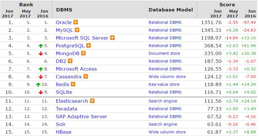
(DB-Engines Rank, 2017)

Database management systems are often classified according to the database model that they support. DBMS types and their period are briefly explained below.

 

 

1960s, navigational DBMS

The introduction of the term database intersects with the availability of direct-access storage from 1960s. The term represented a contrast with the tape-based systems of the past, allowing shared interactive use rather than daily batch processing. The Oxford English Dictionary cites(Wikipedia, n.d.) a 1962 report by the System Development Corporation of California as the first to use the term “data-base” in a specific technical sense.

Since computers evolved rapidly with increased capacity, numerous database systems popped up; by the mid-1960s a number of such systems had used for commercially. Interest in a standard began to grow, and Charles Bachman, author of one such product, the Integrated Data Store (IDS), founded the “Database Task Group” within CODASYL, the group responsible for the creation and standardization of COBOL. In 1971, the Database Task Group delivered their standard, which generally became known as the “CODASYL approach”, and soon a number of commercial products based on this approach entered the market.

The CODASYL approach based on the “manual” navigation of a linked data set which was formed into a large network. Applications could find records by one of three methods:

• Use of a primary key
• Navigating relationships (called sets) from one record to another
• Scanning all the records in a sequential order

1970s, relational DBMS

Edgar Codd worked at IBM. He was pioneered in the development of hard disk systems. He was not satisfied with the navigational model of the CODASYL approach, significantly lack of searching. In 1970, he wrote a number of papers that outlined a new approach to database construction that eventually culminated in the groundbreaking A Relational Model of Data for Large Shared Data Banks.(Codd, 1970)

In this paper, it is described that a new system for storing and working with large databases. Instead of records being stored in some sort of linked list of free-form records as in CODASYL, his idea was to use a “table” of fixed-length records, with each table used for a different type of entity. A linked-list system would be very inefficient when storing “sparse” databases where some of the data for any one record could be left empty. The relational model solved this by splitting the data into a series of normalized tables (or relations), with optional elements being moved out of the main table to where they would take up room only if needed. Data may be freely manipulated with insert, delete, edit and update and so on within these tables, with the DBMS doing whatever maintenance needed to present a table view to the application/user.

In the relational model, records are “linked” using virtual keys not stored in the database but defined as needed between the data contained in the records.

The relational model also allowed the content of the database to evolve without constant rewriting of links and pointers. The relational part comes from entities referencing other entities in what is known as one-to-many relationship, like a traditional hierarchical model, and many-to-many relationship, like a navigational (network) model. Thus, a relational model can express both hierarchical and navigational models, as well as its native tabular model, allowing for pure or combined modeling in terms of these three models, as the application requires.

For instance, a common use of a database system is to trace information about users, their name, login information, various addresses and phone numbers. In the navigational approach, all of this data would be placed in a single record (Figure 2), and unused items would simply not be placed in the database. In the relational approach, the data would be normalized into a subscriber table, a subscriber status table, a phone number table and address table (Figure 3). Records would be created in these optional tables only if the address or phone numbers were actually provided.

Figure 2

Number	Name	Surname	Operator	Upper Package	Package	Status	Address
5374982610	Halil	Baysal	Vodafone	Red	Red L	Connected	Kadikoy

Figure 3

	Number
	Subscriber Key	Number
	537498261020160930	5374982610
	Subscriber
	Subscriber Key	Name	Surname
	537498261020160930	Halil	Baysal
	Package Status
	Subscriber Key	Upper Package	Package	Status
	537498261020160930	Red	Red L	Connected
	Address
	Subscriber Key	Address
	537498261020160930	Kadikoy

Linking the information back together is the key to this system. In the relational model, some bit of information was used as a “key”, uniquely defining a particular record. When data is collected from a specific subscriber number key, data stored in the optional tables can be found by searching for this key whether it is null or not. For instance, if the subscriber number key of a subscriber is unique, addresses, package, name and surname for that subscriber would be recorded with the subscriber key as its key. This simple “re-linking” of related data back into a single collection (basic SQL select statement by joining two tables) is something that traditional computer languages are not designed for.

Just as the navigational approach would require programs to loop in order to retrieve data, the relational approach would require loops to retrieve information about any one record. Codd’s suggestions was a set-oriented language, that would later bring up the ubiquitous SQL. Using a bunch of mathematics known as tuple calculus, he showed that such a system could support all the operations of normal databases (inserting, updating etc.) as well as providing a simple system for finding and returning sets of data in a single operation (known as select statement).

Codd’s paper was chosen by two people at Berkeley, Eugene Wong and Michael Stonebraker. Then INGRES project was started with using funds that had already been reserved for a geographical database project and student programmers to expose code. Beginning in 1973, INGRES delivered its first test products which were generally ready for widespread use in 1979. INGRES was similar to System R in a number of ways, including the use of a “language” for data access, known as QUEL. Over time, INGRES moved to the emerging SQL standard.

IBM itself did one test implementation of the relational model, PRTV, and a production one, Business System 12, both now discontinued. Honeywell wrote MRDS for Multics, and now there are two new implementations: Alphora Dataphor and Rel. Most other DBMS implementations usually called relational are actually SQL DBMSs.

Integrated approach

In the 1970s and 1980s, It was strained that building database systems with integrated hardware and software. Base idea was providing higher performance at lower cost once hardware and software were being integrated. Examples were IBM System/38, the early stage of Teradata, and the Britton Lee, Inc. database machine.

Another idea to hardware support for database management was ICL’s CAFS accelerator, a hardware disk controller with programmable search capabilities. In the long term, these efforts were generally unsuccessful because specialized database machines could not keep dealing with the rapid development and progress of general-purpose computers. Thus, most database systems nowadays are software systems running on general-purpose hardware, using general-purpose computer to store data. However, this idea is still chased for certain applications by some companies like Netezza and Oracle (Exadata).

Late 1970s, SQL DBMS

IBM started working on a prototype system loosely based on Codd’s concepts as System R in the early 1970s. The first version was started on multi-table systems where the data could be split so that all of the data for a record (some of which is optional) did not have to be stored in a single large “chunk”. Subsequent multi-user versions were tested by customers in 1978 and 1979, by which time a standardized query language – SQL– had been added. Codd’s ideas were establishing themselves as both workable and superior to CODASYL, pushing IBM to develop a true production version of System R, known as SQL/DS, and, later, Database 2 (DB2).

Larry Ellison’s Oracle started from a different chain, based on IBM’s papers on System R, and beat IBM to market when the first version was released in 1978.

There were different applications on the lessons from INGRES to develop a new database by Stonebraker, Postgres, which is now known as PostgreSQL. PostgreSQL is often used for global mission critical applications (the .org and .info domain name registries use it as their primary data store, as do many large companies and financial institutions).

In Sweden, Codd’s paper was also read and Mimer SQL was developed from the mid-1970s at Uppsala University. In 1984, this project was joint with an independent enterprise. In the early 1980s, Transaction handling was introduced for high invulnerability in applications that was later implemented on most other DBMSs by Mimer,

Another data model, the entity–relationship model, popped-up in 1976 and become popular for database design as it emphasized a more familiar description than the earlier relational model. Later on, entity–relationship structure was renewed as a data modeling keystone for the relational model, and the difference between the two have become irrelevant.

1980s, on the desktop

The 1980s pioneered in the age of desktop computing. The new computers empowered their users with spreadsheets like Lotus 1-2-3 and database software like dBASE. The dBASE product was slight and easy for any computer user to understand out of the box. C. Wayne Ratliff the creator of dBASE stated: “dBASE was different from programs like BASIC, C, FORTRAN, and COBOL in that a lot of the dirty work had already been done. The data manipulation is done by dBASE instead of by the user, so the user can concentrate on what he is doing, rather than having to mess with the dirty details of opening, reading, and closing files, and managing space allocation.”(Ratliff, 2013)dBASE was one of the top selling software titles in the 1980s and early 1990s.

1990s, Object-Oriented

The 1990s, along with a rise in object-oriented programming, saw a growth in how data in various databases were handled. Programmers and designers started to use the data in databases as objects. That is to say that if a person’s data were in a database, that person’s attributes, such as their address, phone number, package were now considered to belong to that person instead of being external data. This allows for relations between data to be relations to objects and their attributes and not to individual fields. (Database References, 2013) The term “object-relational impedance mismatch” described the inconvenience of translating between programmed objects and database tables. Object databases and object-relational databases are used to solve this problem by providing an object-oriented language (sometimes as extensions to SQL) that programmers can use as alternative to only relational SQL. On the programming side, libraries, object-relational mappings (ORMs), are used to solve the same problem.

2000s, NoSQL and NewSQL

XML databases are a kind of structured document-oriented database which lets querying based on XML document attributes. XML databases are mostly used in enterprise database management, where XML is being used as the machine-to-machine data interoperability standard. XML database management systems include commercial software MarkLogic, Oracle Berkeley DB XML, and a free use software Clusterpoint Distributed XML/JSON Database. All are enterprise software database platforms and support industry standard ACID-compliant transaction processing with strong database consistency characteristics and high level of database security.

NoSQL databases are often very rapid, do not require fixed table schemas, escape join operations by storing denormalized data, and are designed to scale horizontally in other words row count increase is not advised but having more columns in table. The most popular NoSQL systems include MongoDB, Couchbase, Riak, Memcached, Redis, CouchDB, Hazelcast, Apache Cassandra, and HBase which are all open-source software products.

In recent years, there was a high demand for massively distributed databases with high partition tolerance but according to the CAP theorem it is impossible for a distributed system to simultaneously provide consistency, availability, and partition tolerance guarantees. A distributed system can satisfy any two of these guarantees at the same time, but not all three. For that reason, many NoSQL databases are using what is called eventual consistency to provide both availability and partition tolerance guarantees with a reduced level of data consistency which brings to the end reliability of the retrieved data are offered some defined trust rate such as 95% reliability.

NewSQL is a class of modern relational databases that aims to provide the same scalable performance of NoSQL systems for online transaction processing (read-write) workloads while still using SQL and maintaining the ACID guarantees of a traditional database system. Such databases include ScaleBase, Clustrix, EnterpriseDB, MemSQL, NuoDB and VoltDB.

Table is a component in database for collecting of many data entries by being composed of records and fields. Tables are also called as datasheets. There is a basic sample of table (Figure 4) shown below which keeps subscribers’ active addon packages and their activities.

Date	Subscriber	Package ID	Category	Package Name	Opt-in	Opt-out	Active Flag
30.05.2017	59005739920130827	DOV3GBPRP	DOV	Data Over Voice 3GB	1	1	1
30.05.2017	59466160020110421	DOV3GBPRP	DOV	Data Over Voice 3GB	1	1	1
30.05.2017	59414106920170524	TORPDST2GB	DOV	Mazya 2 GB Data Add on	1	0	1
30.05.2017	58059519820110126	DOV10GB110	DOV	Internet 10GB	1	1	1
30.05.2017	59327311920170105	DOV10GB110	DOV	Internet 10GB	1	0	1
30.05.2017	58347936820160413	DOV10GB110	DOV	Internet 10GB	1	1	1
30.05.2017	59059197520161116	DOV10GB110	DOV	Internet 10GB	0	0	1
30.05.2017	59310451520161228	DOV10GB110	DOV	Internet 10GB	1	0	1
30.05.2017	59295348420100628	DOV10GB110	DOV	Internet 10GB	1	0	1
30.05.2017	59302699220160711	DOV10GB110	DOV	Internet 10GB	1	0	1

Figure 4

Record is the place where data is kept. A record is composed of fields and includes all the data about one particular subscriber, address, or package and so on in a database. In this table (Figure 5), a record contains the data for one subscriber id(key) and add-on package being used by him/herself. Records appear as rows in the table.

Date	Subscriber	Package ID	Category	Package Name	Opt-in	Opt-out	Active Flag
30.05.2017	59005739920130827	DOV3GBPRP	DOV	Data Over Voice 3GB	1	1	1

Figure 5

Field is component of a record and contains a single piece of data for the related subject of the record. In the table shown in Figure 5, each record contains 8 fields. Each field, another word columns, are correspondent. They illustrate their related subjects to the database user. It can be seen below. DB user can understand that subscriber field belongs to different subscribers. (Figure 6)

Subscriber
59005739920130827
59466160020110421
59414106920170524
58059519820110126
59327311920170105
58347936820160413
59059197520161116
59310451520161228
59295348420100628
59302699220160711

Figure 6

Filter displays records in a database based on the criteria which is preferred to retrieve. Performance while implementing a filter on the query is dependent on some derivatives such as strength of the server, table size and table creation attributes. To have an imagination, 7-8 million active subscribers in a telecom company generates 350 million (with the size of 128 GB for that partition) data events over base stations within a day. Once there is a filter on this table for a specific subscriber for 6 months, it will not be possible to fetch data even there is Exadata server. In SQL, it is used with a “where” statement.

 

Query finds, inserts, updates records in a database according to request which is being specified.

Report presents data in an understandable format and is especially appropriate for printing, analyzing and forecasting. Reports can display data from tables or queries. All or selected fields can be included in a report. Data can be grouped or sorted and arranged in numerous ways.

2.    Details of Data Warehouse

2.1.  What is Data Warehouse?

It is cited that data warehouse is a database that stores current and historical data of potential interest to decision makers throughout the company. (Kenneth C. Laudon, 2014) The data is generated in many core operational transaction systems, such as systems for CRM, Online Web Services, EMM, TABS, Call Center and Network System transactions. The data warehouse fetches current and historical data from various operational systems, in other words servers, within the organization. These data are combined with data from external sources and transformed by correcting inaccurate and incomplete data and remodeling the data for management reporting, analysis and mining before being loaded into the data warehouse.

Availability of the data is provided by data warehouse system. Data can be reached by anyone based on the requirement but data cannot be changed or edited by these end users. A data warehouse system also provides a range of ad hoc and standardized query tools, analytical tools, and graphical reporting facilities for certain times. This is the significant difference from Big Data. Reachable data for a time range in a data warehouse environment is not as wide as in Big Data environment.

2.2.  Data Warehouse Concepts in Telecommunication

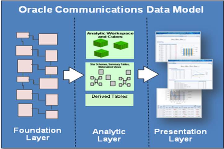
Mainly the idea of the OCDM

2.2.1.     Source System

2.2.2.     Staging Area

2.2.3.     DWH Layers in Telecommunication

2.3. Significant Terms in Data Warehousing

2.3.1.     Granularity

Granularity definitions have various answers. Les Barbusinski’s Answer: Granularity is usually mentioned in the context of dimensional data structures (i.e., facts and dimensions) and refers to the level of detail in a given fact table. The more detail there is in the fact table, the higher its granularity and vice versa. (Joe Oates, 2002) In another word, once there is the higher granularity of a fact table, count of rows will be closed to the transaction level.

For example, there is a DataMart which has time, cell station (Region & City), call direction (incoming or outgoing), call type (international and local), event type name (voice call, SMS, data, MMS, and VAS) and metric values such as usage revenue, data consumption, calling duration, free SMS events.

Though dimensions of the any CDR for sure do not consist of listed dimension previously. A CDR has more dimensions like Package dimension which includes subscription type of any main package being used by the customers. The metrics in the Cell fact table must be stored at some intersection of the dimensions (i.e., Time, Cell, Call Direction, Call Type, and Event Type) based on the need, even though there is a chance to have more details on traffic events in other word higher granularity. This may be helpful to increase the depth of the analysis. On the other hand, there will be surely performance issues while fetching the data by increasing row counts and scanning more rows. For a real estimation, there are 350 million data events within a day at the most atomic (granular) level because it includes not only the date of event but also timestamp of the event. (This one day data event data is around 128 GB without compression) Once a subscriber wants to read data for 20 days, it will be an issue for database while bringing the results. Also, end users are not searching only for data events they are also looking for SMS, MMS and Voice Call Events. Once traffic events are all gathered at the highest granularity, row count for one day traffic events is around 450 million. There is no such a way to call this raw data as an analysis. That is why granularity has to be specified. Once time dimension is changed from day with timestamp detail to day detail, row count of the specified may be decreased to 100 million. It is still raw data but can be analyzed.

Chuck Kelley’s, Joe Oates’, and Clay Rehm’s answers are more or less similar with Les Barbusinski’s. In order to call any analysis to make decisions, it shouldn’t be based on raw data. It should be adjusted, specified, and aimed to accurate target. This is called as an analysis upon Business Intelligence terms and granularity is one of the significant component of this terms.

2.3.2.     Normalization

Normalization is a process of organizing the data in database to avoid data redundancy, and any anomalies. There are three types of anomalies that may occur when the database is not normalized. These are insertion, update and deletion anomalies.

To illustrate, manufacturing company which stores the employee details in a table named employee having four attributes: emp_id for storing ID, Name for employee’s name, Address for address  of employee’s and Department for the department details in which the employee works. Basically, tabel is shown below. (Table 1)

Table 1

ID	Name	Address	Department
101	Ahmet	Aydın	D001
101	Ahmet	Aydın	D002
123	Veli	Denizli	D890
166	Hatice	Kayseri	D900
166	Hatice	Kayseri	D004

Table 1 is not normalized. There are three kinds regarding this problem.

Update anomaly: In Table 1, There are two rows for Name Ahmet as he belongs to two departments within the company. If it is required to update the address of Ahmet then there is  update the same in two rows or the data will become inconsistent. If somehow, the correct address gets updated in one department but not in other then as per the database, Ahmet would be having two different addresses, which is not possible and would lead to inconsistent data.

Insert anomaly: There is a new hired worker who is under training and currently not directed to any department. There is no way to insert the data into the table if department field doesn’t allow null attribute.

Delete anomaly: It can be supposed that if the company stops operations of the department D890 in certain period of time, then deleting the rows which are having department as D890 will also remove the information of employee Veli because he is dedicated himself only to this department.

In order not to face with these anomalies, tables have to normalized. There are many types of normalization. Common ones are shown below.

• First normal form(1NF)
• Second normal form(2NF)
• Third normal form(3NF)
• Boyce & Codd normal form (BCNF)

First normal form (1NF) can be declared as an attribute (column) of a table cannot keep multiple values. It should keep only atomic values.

Supposingly, a company wants to hold the names and contact of its employees. It creates a table that looks like this:

ID	Name	Address	Phone
101	Ali	Denizli	8912312390
102	Veli	Kayseri	8812121212 9900012222
103	Ayse	İstanbul	7778881212
104	Can	Trabzon	9990000123 8123450987

Table 2

Two employees (Veli & Can) have two phone numbers therefore the company stored them in the same field in Table 2.

This table is not in 1NF rules. Rule is defined as “each attribute of a table must have single values”, phone number values for employees Ali & Can violates that rule.

To make the table get along with 1NF, this table should be transformed in Table 3.

emp_id	emp_name	emp_address	emp_mobile
101	Ali	Denizli	8912312390
102	Veli	Kayseri	8812121212
102	Veli	Kayseri	9900012222
103	Ayse	Istanbul	7778881212
104	Can	Trabzon	9990000123
104	Can	Trabzon	8123450987

Table 3

Second normal form (2NF) tables should be based on two rules below.

• Table should be in 1NF (First normal form)
• No non-prime attribute is dependent on the proper subset of any candidate key of table.

An attribute which is not part of any candidate key is defined as non-prime attribute.

For example, a school wants to store the data of instrcutors and the areas they have knowledge. Being created table might seem in Table 4. Since an instructor can teach more than one subjects, the table can have multiple rows for the same instructor.

ID	Subject	Age
111	Maths	38
111	Physics	38
222	Biology	38
333	Physics	40
333	Chemistry	40

Table 4

Candidate Keys are ID and Subject.Non prime attribute is Age in Table 4. The table is in 1 NF because each attribute has single values. However, it is not in 2NF because non prime attribute teacher_age is dependent on teacher_id alone which is a proper subset of candidate key. This violates the rule for 2NF as the rule says “no non-prime attribute is dependent on the proper subset of any candidate key of the table”.

To make the table complies with 2NF, it has to be divided into two tables like below tables;
Teacher details table (Table 5)

ID	Age
111	38
222	38
333	40

Table 5

Teacher subject table (Table 6)

teacher_id	subject
111	Maths
111	Physics
222	Biology
333	Physics
333	Chemistry

Table 6

After dividing tables into 2 tables, the ruke for the second normal form (2NF) is achieved.

Third Normal form (3NF)

There are some certain rules to accept any table as 3NF if both the following conditions are provided below:

• Table must be in 2NF
• Transitive functional dependency of non-prime attribute on any super key should be existing.

In another words, 3NF can be defined as in 3NF if it is in 2NF and for each functional dependency X over Y at least one of the following conditions hold:

• X is a super key of table
• Y is a prime attribute of table

For example, a company wants to keep the complete address of each employee, employee_details table is created as below.

ID	Name	Zip	State	City	County
1001	Refik	282005	TR	Denizli	Kuspinar
1002	Mert	222008	UK	London	Nicaragua
1006	Halil	282007	TR	Istanbul	Istiklal
1101	Cem	292008	IT	Milano	Lux
1201	Can	222999	TR	Kayseri	Cinar

Table 7

Super keys: {ID}, {ID, Name}, {ID, Name, Zip}…so on
Candidate Keys: {ID}
Non-prime attributes: all attributes except ID are non-prime as they are not part of any candidate keys.

In this example, City and County are dependent on Zip. Zip field is dependent on ID that makes non-prime attributes (state, city and County) are transitively dependent on super key which is ID. This violates the rule of 3NF. To make this table complies with 3NF, It has to be divided into two tables to remove the transitive dependency:

Employee ID table (Table 8):

ID	Name	Zip
1001	Refik	282005
1002	Mert	222008
1006	Halil	282007
1101	Cem	292008
1201	Can	222999

Table 8

Zip table (Table 9):

Zip	State	City	County
282005	TR	Denizli	Kuspinar
222008	UK	London	Nicaragua
282007	TR	Istanbul	Istiklal
292008	IT	Milano	Lux
222999	TR	Kayseri	Cinar

Table 9

Boyce Codd Normal Form (BCNF)

It is an advance version of 3NF. It is also called as 3.5NF. BCNF is stricter than 3NF. A table complies with BCNF if it is in 3NF and for every functional dependency X over Y, X should be the super key of the table.

To illustrate, there is a company where employees can work in more than one department. Made up table is shown below (Table 10).

ID	Nation	Department	Dept Code	Dept No of Employee
1001	Turkish	Production and planning	D001	200
1001	Turkish	Stores	D001	250
1002	Jamaican	Design and technical support	D134	100
1002	Jamaican	Purchasing department	D134	600

Table 10

Functional dependencies in Table 10:

ID over Nation

Department over Dept Code and Dept No of Employee

Candidate key: {ID, Department}

Table 10 is not in BCNF as whether ID and Department are keys. To change the table to comply with BCNF, It has to be divided into three tables;
Nationality table:

emp_id	emp_nationality
1001	Turkish
1002	Jamaican

Table 11

Department table:

Department	Department Code	Dept No of Employee
Production and planning	D001	200
Stores	D001	250
Design and technical support	D134	100
Purchasing department	D134	600

Table 12

Employee to Department table:

ID	Department
1001	Production and planning
1001	stores
1002	design and technical support
1002	Purchasing department

Table 13

Functional dependencies:

ID over Nationality, Department over { Dept Code, Dept No of Employee }

Candidate keys are ;

• For first table: ID
• For second table: Department
• For third table: ID and Department.

This is transformed to the BCNF since both the functional dependencies left side part is a key.

2.3.3.     Denormalization

Denormalization is a strategy used on a previously-normalized database to increase performance. The logic behind is to add excess data where it will be beneficial the most. It can be used for extra attributes in an existing table, add new tables, or even create instances of existing tables. The general purpose is to decrease the execution time of select queries by increasing the accessibility of data to the queries or by populating summarized reports in separate tables. (Drkušić, 2016)

Decision criteria to denormalize the database;

As with almost anything, reasons to apply denormalization progress have to assessed. It has to be guaranteed that profit will be generated by decreasing the risks.

Maintaining history is the first reason for denormalization. Data can change during time, and surely values have to be stored that were valid when a record was created. For example, a person’s address or mobile number can be changed or a client can change their business name or any other data. Once they are generated, they should be included. Otherwise populating historic data for a certain period may not be possible. It can be solved by adding a timestamp for the transactions. It increases the query complexity surely but it will be used in that case.

Second reason is to improve query performance. Some of the queries may use multiple tables to access data that is needed frequently. Think of a situation where there is a need to join 10 tables to return the client’s sales channel representative and the region where products are being sold. Some tables along the path may contain large amounts of data. In this sort of case, it would be wiser to add a subscriber id attribute directly into the sales channel table.

Third reason is to boost reporting execution period. Creating reports from live data is quite time-consuming and can affect overall system performance (big data’s big problem). Let’s say that it is required to track client sales over certain years for all clients in a requirement. Generating such reports out of live data would “dig” almost throughout the whole database and slow it down a lot because of the consumed storage on RAM and processors. Computing commonly-needed values up front: Having values ready-computed so it is not required to generate them in real time.

It’s important to understand that use of denormalization may not be required if there are no performance issues in the application. Yet, if there is any notice that the system is slowing down – or may happen – then applying of this technique can be discussed.

Disadvantages of Denormalization;

Obviously, the biggest advantage of the normalization process is increased performance. Yet, it comes with many drawbacks listed as below.

• Higher disk space need is one of the concern because there is duplicated data on some attributes.
• Data anomalies is another disadvantage of using denormalization. It requires a lot of attention. Since, data is not populated only from a one source. It has to be adjusted every piece of duplicate data accordingly. That is also applied to reports. In order not to, face with these sort of issue, adjustment of the model has huge importance.
• Documentation increase for each denormalization rule that is being applied. If database design is modified later, at all our exceptions and take them into consideration once again.
• Slowing down other operations is another drawback. It can be expected that there is slowness while data insert, modification, and deletion operations. If these operations happen merely, this could be a benefit. Simply, there will be one division for slow select into a larger number of slower insert/update/delete queries. While a very complex select query technically could slows down the entire system, slowing down multiple “smaller” operations should not affect badly the usability of applications.

To sum up, there are more significant indicators while using normalized or denormalized approaches. Normalized databases work very well under conditions where the applications are write-intensive and the write-load is more than the read-load. Updates are very fast. Inserts are very rapid because the data has to be inserted at a single place and does not have to be duplicated. Select statements are fast in cases where data has to be retrieved from a single table, because normally normalized tables are small enough to get fit into the buffer. Although there seems to be numerous advantages of normalized tables, the main cause of concern with fully normalized tables is that normalized data means joins between tables. Join operation means that reading have to suffer since indexing strategies do not go well with table joins. Denormalized databases works well under heavy read-load and when the application is read intensive. This happens because of the following reasons; data is present in the same table so there is no need for any joins, this lead “select statements” to become very fast. More efficient index usage is another key benefit of this approach. If the columns are indexed properly, then results can be filtered and sorted by utilizing the same index. While in the case of a normalized table, since the data is spread out in different tables, this would not be possible. Although select statements can be very fast on denormalized tables, but because the data is duplicated, DMLs (updates, inserts and deletes) become complicated and costly. It is not possible to neglect one of the approach while comparing with other one.  In real world application, both read-loads and write-loads are required.  Correct way would be to utilize both the normalized and denormalized approaches depending on the cases being required.

2.3.4.     Aggregation

Aggregation is another important component within DWH systems. There is always calculation for computable attributes. These attributes consist of KPIs, in other words fact, measure or metrics. (It will be explained within details in Fact section). Within an analysis, there is always need for the aggregation functions in order to understand the data based on the grouped by attributes. (It will be explained within details in Dimension section.) For example, based on cell station, call type and call direction summing the data being used, revenue being generated. This sample table is shown below.

Cell Station	Call Type	Call Direction	Data Size	Usage Revenue
12	International	Incoming	0	1
13	International	Outgoing	0	3
14	Local	Incoming	0	4

Table 14

There are many functions for Aggregations. Sample functions are shown below;

• Average
• Count
• Maximum
• Nanmean
• Median
• Minimum
• Mode
• Sum

2.3.5.     Dimension

A dimension is a structure that divides facts and measures in order to enable users to answer business questions, make their analysis and transform data to information -assigning a meaning to data-. Commonly used dimensions are products, location, time, subscriber and so on in telecommunication.

In a data warehouse, dimensions provide structured labeling information to otherwise unordered numeric metrics. The dimension is a data set composed of individual, non-overlapping data elements. The primary functions of dimensions are threefold: to provide filtering, grouping and labelling. (Wikipedia Org., 2017)

2.3.6.     Fact

A fact is a value or measurement which represents a fact about the managed entity or system. In other words, metrics -fact- are calculated values by using aggregation function. For example, the ratio of profitability of Vodafone Red L subscribers, average revenue per user (ARPU), possible churn rate of the subscriber and so on.

In order to distinguish terms of Fact and Dimension. Below table can be used as indicator of both.

Cell Name	Data Usage Amount	Data Usage Size MB
Bostanci-1	12.321,12	12.391.390,12
Bostanci-4	9.340,22	123.213,00
Kadikoy-1	12.312,40	9.890.889,30
Kadikoy-2	73.872,20	9.090.112,20
Kadikoy-3	98.194,09	9.090.122,20
Kadikoy-4	3.123,20	965.612,20
Kadikoy-5	93.828,81	78.560.112,20
Atakoy-4	123.123,30	45.612,20

Table 15

Cell Name is the dimension of the table. Metric values are grouped by Cell Name. It shows the Data Usage Amount which is the charged amount for the data events and Data Usage Size MB which is the total data consumed in MB based on Cell Name dimension.

2.4. ODI as a Tool of Data Warehousing

Oracle Data Integrator -ODI- is used for extracting data from different source systems such as Attunity, Axis2, BTrieve, Complex File, DBase, Derby, File, Groovy, Hive, Hyperion Essbase, Hyperion Financial Management, Hyperion Planning, Hypersonic SQL, IBM DB2 UDB, IBM DB2/400, In-Memory Engine, Informix, Ingres, Interbase, JAX-WS, JMS Queue, JMS Queue XML, JMS Topic, JMS Topic XML, Java BeanShell, JavaScript, Jython, LDAP,              Microsoft Access, Microsoft Excel, Microsoft SQL Server, MySQL, NetRexx, Netezza, ODI Tools, Operating System, Oracle, Oracle BAM, Oracle BI, Paradox, PostgreSQL, Progress, SAP ABAP,              SAP Java Connector,              SAS (deprecated), Salesforce.com (deprecated), Sybase AS Anywhere, Sybase AS Enterprise, Sybase AS IQ, Teradata, TimesTen, Universe, XML and loads data into modelled tables while transforming. It is an ELT tool. This makes ODI unique while comparing with the other Data warehousing tools like Informatica (IBM’s DWH tool)

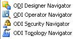
There are four main windows once ODI is opened which is shown below.

Figure 7

Designer Navigator is used to design data integrity checks and to build transformations such as for example:

• Automatic reverse-engineering of existing applications or databases
• Visual development and maintenance of transformation and integration interfaces
• Visualization of data flows in the interfaces
• Automatic documentation generation
• Customization of the generated code

Figure 8

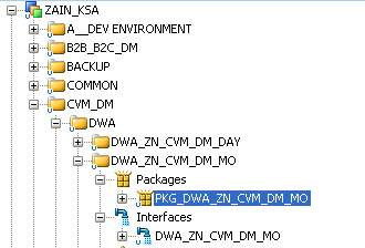
In Figure 8, there is project section of Designer which includes directories of the development.

Figure 9

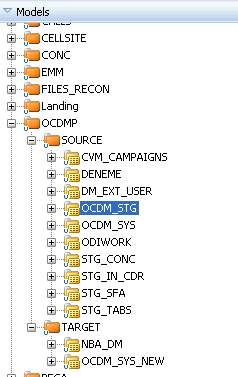
In Figure 9, It shows the defined schemas and their tables as model. It is used for reverse engineering the created databases and their tables.

Figure 10

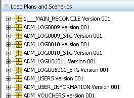
In Figure 10, there are the scenarios of the developed interfaces and packages. These scenarios are xml files which have defined data load flow, variables and package or interface details.

Figure 11

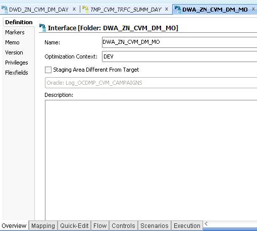
In Figure 11, there is a window of an interface which has an overview tab it includes definition to give a name to the interface, optimization context which is used for executing scripts on specified database and logical schema. Version shows the date of creation and update of the interface.

Figure 12

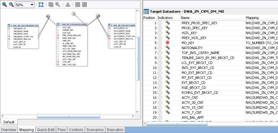
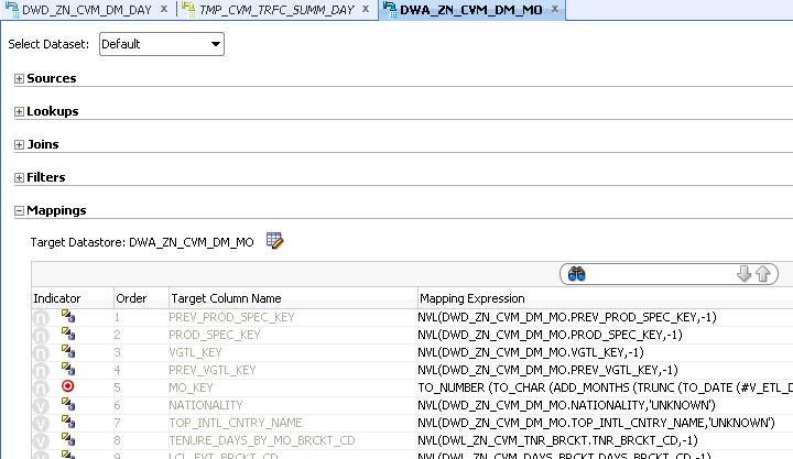
In Figure 12, there is definition of the mapping rules on target table’s columns. Source tables which are used for loading this target table are dragged in to the white panel on the left. Joins can be defined by dragging columns to another column (foreign key) in other table. Filters are defined by dragging the required column out of the boundaries of table surface.

On the right panel, there is name of the target data store. ‘DWA_ZN_CVM_DM_MO’ in our case. Target is defined in model and attributes of the table are filled by the mapping rule from the source.

Figure 13

In Figure 13, Quick Edit tab is shown. This tab identically is used for the operations can be done in Mapping. Source to define source tables. Joins to define join conditions between source tables. Filters to define filter rules. Mapping to define how to load data on target table’s attributes. Target data store shows the database objects where ELTs are loaded through.

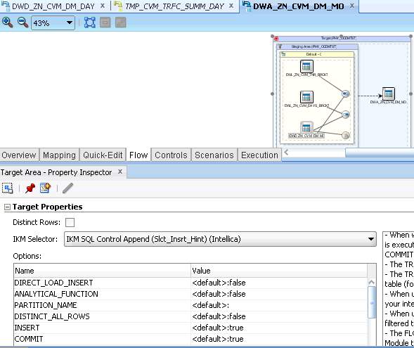Figure 14

In Figure 14, data flow preview can be seen as above. Also, knowledge module selection can be adjusted in this panel. Knowledge modules are scripted modules that contain database and application-specific patterns. There are many types of Knowledge modules. Mainly, they are shown as below.

Loading Knowledge Module (LKM) is used to load data from a source datastore to staging tables. This loading can be referred that when some transformations take place in the staging area and the source datastore is on a different data server than in the staging area.

Integration Knowledge Module (IKM) is another type of KMs. It takes place in the interface during an integration process to integrate data from source or loading table into the target datastore depending on selected integration mode; insert, update or to capture SCD.

In our example, IKM is used. There are parameters while using this KM. Benefits of the KMs can be observed. KMs are extensible. If any change occurs in Interfaces, KM is modified and covers the newly emerged needs. In this KM, creation of the target table, truncation of target and that sort of parameters can be set based on the need.

Operator Navigator is the management and monitoring tool to follow ETLs’ success or time consumption. It is designed for IT production operators. Through Operator Navigator, interface or package scenario executions can be traced in the sessions, as well as the scenarios.

Figure 15

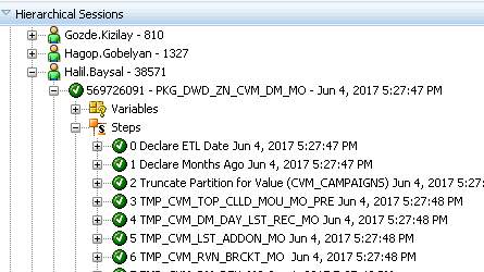
In Figure 15, It can be seen that execution of the package is done successfully. Steps define the que of the pre-steps in this package in order to load the target table accurately.

Topology Navigator is used to manage the data describing the information system’s physical and logical architecture. By Topology Navigator, the topology of your information system, the technologies and their datatypes, the data servers linked to these technologies and the schemas they contain, the contexts, the languages, the agents, and the repositories can be managed. The site, machine, and data server descriptions let Oracle Data Integrator to execute the same integration interfaces in different physical environments.

Figure 16

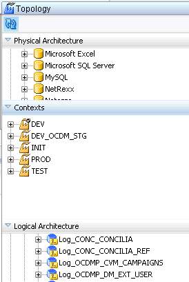
In Figure 16, Physical Architecture is used for defining the technology type of the source databases. Contexts are bridge between production and development in the case above. If DEV is chosen data load will be executed in Development Environment. Logical Architecture is conductor of the schema which is pointed.

Security Navigator is the tool for implementing the security rules in Oracle Data Integrator. By Security Navigator, users and profiles and assign user rights for methods (edit, delete, etc) on generic objects, and fine-tune these rights on the object instances can be created.

Sample Case:

Add-on department business end users wants to retrieve daily add-on packages subscription based on main packages.

Solution for this requirement is simple. In order to have that analysis there is a table which keeps historic data at the most atomic level. In other words, once a subscriber opts in any add-on package any time, a row will be inserted for that transaction. They are not volunteer to have this raw data, as it is not feasible to understand this data. That is why opt-ins, opt-outs, transaction and active base counts for any subscriber have to be identified in a temporary table. After this preparation step is done, subscribers’ opt-ins, opt-outs, transaction and active base counts can be aggregated -being summed- based on the main and add-on package.

Illustration of the solution on ODI are shown below;

Figure 17

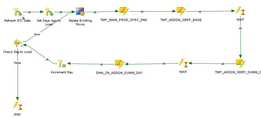
In Figure 17, structure of the current package for daily addon analysis is provided. First step is defining “Refresh ETL Date” variable to start the loop. This variable is provided once this package is executed. It defines the last day to loop this package ETL. “Set Days Ago to Load” is another manually provided variable on execution time. It defines how many days to loop back. Delete Existing Rows is a procedure that removes data for specified dates in order to prevent from duplications in case of reloading on “Addon Summary Daily Analysis”. Then there is another step TMP_MAIN_PROD_SPEC_RNK which is used for ranking the subscriber and subscribers’ main packages on specified date. TMP_ADDON_SBRP_BASE is also another temporary step which loads data for specified date and keeps data of the transactions based on subscriber and package level. WAIT step is quite significant to differentiate the interfaces whether running sync or not. After both temporary preparation steps are done, another temporary table TMP_ADDON_SBRP_SUMM_DAY is started. This scenario is referred to combination of two temporary preparation step previously. This is filled with subscribers, their main packages, their addon packages and start and end date of the addon packages. Lastly, DWA_ZN_ADDON_SUMM_DAY is started by the package automatically. It implements rule basically, if start date equals to the day that package is started then opt in count will be 1 and it will be summed based on main and addon package. Likewise opt-out, active base and transaction count are calculated in the same logic.

3.    Details of Business Intelligence

3.1. What is Business Intelligence?

3.2. History of Business Intelligence

3.3. Significant Terms in Business Intelligence

3.3.1.     Snowflake and Star Schema Definitions and Comparisons

3.3.2.     Dimension Tables

3.3.3.     Fact Tables

3.4. OBIEE as a Tool of Business Intelligence

3.4.1.     Installation of OBIEE

3.4.2.     Creating Repository in OBIEE

3.4.3.     OBIEE Layers

3.4.3.1.             Physical Layer

3.4.3.2.             Business and Mapping Layer

3.4.3.3.             Presentation Layer

3.4.4.     Variables

3.4.5.     OBIEE Reporting Objects

3.4.5.1.             Analysis

3.4.5.2.             Filters

3.4.5.3.             Graphs

3.4.5.4.             Dashboard

4.    Conclusion

5.    References

Codd, E. F. (1970, June). RDBMS. (P. BAXENDALE, Ed.) Communications of the ACM, 13(6), 377-387. Retrieved from Penn Engineering: http://www.seas.upenn.edu/~zives/03f/cis550/codd.pdf

Drkušić, E. (2016, March 17). Vertabelo Blogs. Retrieved May 24, 2017, from Vertabelo Blogs: http://www.vertabelo.com/blog/technical-articles/denormalization-when-why-and-how

Joe Oates, C. K. (2002, June 25). Information Management. Retrieved May 24, 2017, from Information Management: https://www.information-management.com/news/what-does-granularity-mean-in-the-context-of-a-data-warehouse-and-what-are-the-various-levels-of-granularity

Kenneth C. Laudon, J. P. (2014). Management Information Systems: Managing the Digital Firm (13 ed.). Edinburgh Gate, Harlow, England: Pearson Education. Retrieved June 04, 2017

Merriam-Webster. (n.d.). Retrieved from Merriam-Webster: www.merriam-webster.com/dictionary/database

Rank, D.-E. (2017, June). Solid-IT. Retrieved 06 04, 2017, from Solid-IT: https://db-engines.com/en/ranking

Ratliff, C. W. (2013, 07 12). Interview with Wayne Ratliff. Interview with Wayne Ratliff. (T. F. History, Interviewer) Retrieved from http://www.foxprohistory.org/interview_wayne_ratliff.htm

Wikipedia. (n.d.). Retrieved 05 21, 2017, from https://en.wikipedia.org/wiki/Database

Wikipedia. (2013). Retrieved 05 21, 2017, from Wikipedia Org.: https://en.wikipedia.org/wiki/Database#CITEREFNorth2010

Wikipedia Org. (2017, April 5). Retrieved May 19, 2017, from Wikipedia Org.: https://en.wikipedia.org/wiki/Dimension_(data_warehouse)