Dynamic Modeling and Experimental Validation of Direct Contact Membrane Distillation (DCMD)

Dynamic modeling and experimental validation of Direct Contact Membrane Distillation (DCMD) using Computational fluid dynamics using and simulations

ABSTRACT

Direct contact membrane distillation (DCMD) process was modeled using algebraic and computational fluid dynamics methods. These modeling approaches have beneficial outcome in terms of optimization of heat flux, mass flux and fluid flow through DCMD. Two modeling approaches are used for getting results in form of COMSOL (which is CFD tool) and MATLAB based one dimensional algebraic simulation. Graphical user interface (GUI) has provided user friendly method to process the results using computational means and extract numerical data required for calculation. From tools (1) MATLAB results were compared quantitively and (2) CFD results were both qualitively and quantitively analysed. Simulated parameters were optimized using Monte Carlo simulation in MATLAB. A script following user input was used to obtain interfaces temperatures of membrane with feed and permeate. These temperatures were further used to calculate dusty gas parameters. The temperature dependence of process, velocity, pressure, flux magnitudes were shown by numerically obtained results. Present work showed evaluation of Willmott index (d) as 0.9889 and Relative Error (RE) as 0.1304. In this study results found were better, marginal deviation in values of dimensionless numbers (Reynolds and Prandlt), vapour pressures, conductivity and temperature compared to reported literature were seen. Analogy between heat and mass transfer has been established for calculating dimensionless number along DCMD module. Flux obtained was 27 kg/m².hr at 60 degree Celsius with dimension of 15 mm length, 2 mm width and 3 mm depth of the channel for feed and permeate. Trade-off between conductivity and heat transfer coefficients was shown.

Keywords– DCMD; Modeling; CFD; GUI; Simulation; Parameters; Trade-off; Analogy

1. Introduction

Membrane distillation (MD) is an emerging technology for separations that are traditionally accomplished by conventional processes such as distillation or reverse osmosis. It is a thermally driven process in which only vapour molecules are transported through porous hydrophobic membranes.

In membrane distillation, selection properties of the membranes not only effects heat, mass and fluid transport phenomena but also operating conditions, design considerations and distance between spacers. For improving fluid transport, hydrodynamics plays an important role and provide ways to study parameters which effects DCMD process using equations. Equations used by Gilron et al. [19] has been crucial in relating hydrodynamics with vapour pressure. Vapour-liquid equilibrium studies says vapours across the membrane are driven by vapour pressure differences which is the only mode for mass transfer in DCMD.

Modeling steps for heat transfer consisting algebraic equations were taken by Tzahi et al. [1]. Graphical interface in COMSOL was given input as closure relationship. Closure relationships helped to calculate interdependent parameters using CFD simulations carried out by Guhan et al. [2]. Yu et al. studied ways to set up the boundary conditions and making computer aided drawings (CAD) on AUTOCAD for CFD compatible geometry.

Direct contact membrane distillation modules have been created as a mimic of experimental setup. These process parameters which are geometries and flow conditions of feed and permeate etc. were generated virtually using COMSOL. Based on study auxiliary units like condenser, heater, pump and vacuum were created as per respective DCMD process.

Suitable design of the module, process parameters and properties of DCMD membrane reported by Yu et al. [6] and Tzahi et al. [1] has been manipulated and reiterated using MATLAB script to attain a final converged value. Absolute error less than 0.001 was the condition for convergence. A compromise between increased membrane permeability and decreased thermal resistance (which tend to reduce heat efficiency or interface temperature difference) [9] was related to optimum membrane thickness. Although much work had been done in area of fabrication of novel membranes to attain suitable hydrophobicity, porosity and conductivity for DCMD applications, little work has looked at improving design and hydrodynamics. To the best of our knowledge the combined usage of CFD and script based MATLAB modeling studies were limited and thus motivated us to carry out the same for membrane distillation.

Aim behind performing these simulations was to study effects of change of vapour pressure and temperature with brine solution as feed in DCMD module. Two dimensional modelin [6] was developed based on energy, mass and momentum balances same approach has been used in carrying out this study. The results reported for permeate and feed side are calculations in form of dimensionless entities, pressures, conductivity and flux etc.

Current study included  one dimensional algebraic Dusty gas model using Monte Carlo simulation [14] and two dimensional CFD modeling for horizontal and vertical DCMD module with counter current feed/permeate flow. Computational work has not been carried out in the field of DCMD, here it combines analytical, numerical as well as computational ways to study membrane distillation.

Design of direct contact and air gap membrane process by combined usage of Monte Carlo simulation and CFD was found to be a better way of analysing phenomena occurring in the module. Segregation of individual process phenomena was done in three different sections called as feed section, permeate section and membrane. Set of equations on MATLAB were solved for each section which provided optimization of important parameters needed to maintain the required temperature and pressure using an algorithm [13]. Script was reiterated to study effect of change on operating range, geometry etc. which was easy to customize and analyse DCMD process section wise.

This paper studied effect on Dusty gas parameters with respect to laminar, turbulent flow regimes, surface energy, thermal conductivity and porosity [30], [31], [32]. Analysis over temperature polarization coefficient (TPC) along vertical cross section of DCMD module [29], [30],[33] . Effect of temperature gradient on membrane interface temperature and DCMD performance due to dimensionless quantities (Reynolds number, Prandlt number) have been highlighted [25],[31]

Comparison of experimental and predicted flux using Monte Carlo Simulation and effect of module length/diameter on heat transfer coefficient [11], [12] flow distribution with respect to arc length were carried out to analyse DCMD efficiency.

To ensure successful and economical operation experimental validation were performed, Tzahi et al. provided data for validation. Analogy between heat and mass transfer following DCMD, AGMD with laminar flow were suggested [26]

Current study suggested that CFD gives qualitative predictions of length and diameter that influences the MD performance as discussed in [3]. This work in future can be used as a guidance in performing studies on module design, module scale up and process optimization.

Material and Methods

1. Schematic representation and explanation

For determining which turbulent model most accurately represents membrane distillation module flow, heat and mass transfer are coupled at different flow regimes which are laminar, transitional and turbulent, three flow models are chosen for the simulations. They are laminar, k-epsilon and Menter SST k- omega turbulence model.

In membrane distillation, coupling of three different  multi-physics have been carried out which include stationary fluid flow, heat transfer in module and porous media, reaction engineering physics without any reaction, generation and accumulation terms. An isometric behaviour is assumed which enables uniform mixing in both channels on both side of the membrane. The feed temperature, T_f decreases initially and attains a steady value which is T_fm at the interface. Water evaporates from the saline water (Brine) and diffuses through the membrane. Simultaneously, heat is conducted through the membrane to the permeate which is maintained at condensation point. The cold flow temperature T_p rises to follow the boundary layer to attain T_pm at the membrane surface on the cold side. The driving force is therefore, the vapour pressure difference between T_fm and T_p, which is less than the vapour pressure difference between T_f and T_p. This process is called temperature polarization. The temperature polarization coefficient is defined by Schofield et al.[8]as

TPC=Tfm-TpmTf-Tpwhich is to be studied in this work. The diagrammatic representation of vertical and horizontal DCMD module is shown in Figure 2.1(a) and Figure 2.1(b).

  

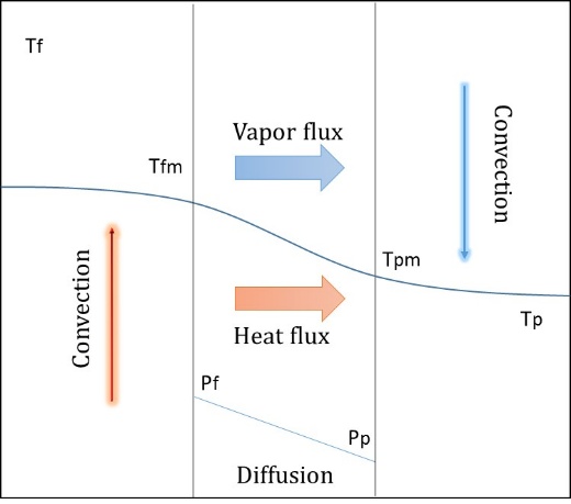
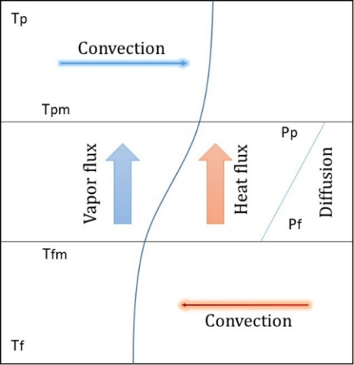
2.1 (a)      2.1 (b)

Figure 2.1-Temperature used in calculation of TPC with flow directions of    feed, permeate, vapour and heat flux with Pressure gradient

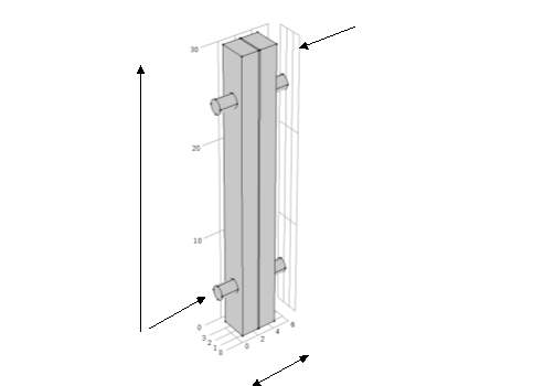
In horizontal module, one tank is mounted on other with diameter of 3 cm and height of 2 cm each as shown in Figure 2.3 and Figure 2.1 (b). Other as vertical geometry with rectangular column of 30 mm height, 3 mm depth and 2mm width for feed and permeate each as shown in Figure 2.2 and Figure 2.1 (a). To analyse in details about the effects of change in various parameters we perform two types of simulations (A) Monte Carlo simulations which took user input of temperatures on bulk side of feed (brine solution) and permeate (pure water). Anonymous values for both interface temperatures were taken as input which gets converged to an optimum value.

(B) Input between 1.75 m/sec to 5 m/sec and Monte Carlo simulation were performed over data provided as input. The average of the outcome was then taken and compared with reported literature by Tzahi Cath Adams et al. [1].

90 numerical simulation using computational tools were performed to compare the results qualitatively and quantitively as shown in figure 3.1 and Figure 3.4.

In Figure 2.3, Saline water flows at 60^oC through the inlet feed from lower end and inlet permeate cold water is fed at 20^oC from the permeate side pump, the temperature is maintained at 40^oC and 20^oC, on the feed and permeate side membrane interfaces with bulk liquids. The velocities are in a range of 1.75m/sec to 5m/sec. Vacuum is applied to the membrane. Temperatures and pressure measuring instruments are used for measurement purpose. Pumps are used according to capacity required..

Figure 2.2–Vertical geometry drawn using SALOME with dimension as depicted by Tzahi Cath et al. in [1]

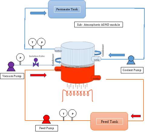
Figure 2.3-Schematic representation of the process

2. Equations and material

The heat transfer model can be made equivalent to an electrical analogy [8] and these equations are best explained and applied if divided into three major divisions: feed, membrane and permeate, separately a set of equations is applied individually as three different entities. The governing equations used are taken from[9] for computational fluid dynamics. COMSOL and ANSYS user manuals were also utilized. Properties used for materials which are water, high strength alloy steel, Air and PEEK (Porous Solid) are directly imported from libraries available in proprietary product COMSOL and Perry’s handbook. Here speed of sound is used at certain places for numerically solving the discretized domain. The equations used for simulations are as follows-

Continuity Equation-

∂ρ∂t+∇.(ρv⃗)=0      —— (1)

Navier Stokes Equation-

∂(ρv⃗)∂t+∇.ρv⃗v⃗=-∇p+∇.τ̿+ρg⃗+F⃗  —— (2)

Energy Equation-

ρCp∂T∂t+u.∇T=-∇.q+ τ:S-Tρ∂ρ∂tp∂P∂t+u.∇p+Q ——- (3)

Stress Tensor-

τ̿= μ[∇v⃗+∇v⃗T-23∇.v⃗]      —— (4)

Darcy‘s law-

∂Vp∂t=J=∆pμA(1Rm+R)       —— (5)

Reynolds (Re) and Prandlt (Pr) Number for both permeate and feed side-

Re=Dvρμ

and

Pr=Cpμk     —— (6)

Nusselt Number-

Nu=1.86×Pr×Re×DiaL0.33 —— (7)

Heat transfer coefficient (h) of both permeate and feed boundary layer-

h=Nu×kD

—— (8)

Dittus-Boelter Equation-

h=1+6DiameterLp×0.023×Pr0.33×Re0.8——9

Knudsen diffusion coefficient of the water vapour-

Dk=23r8RTπM12—–(10), here R= 8314 known as universal gas constant,

τis 1.8 and molecular weight of water has been used in place of M.

General flux-

Ji∆p=23 Dk1RTrεLp+p̅8μiRTr2εLp, —— (11), here second term denotes mass transfer due to Poiseuille’s flow and first denotes Knudsen diffusion taken from [21].

3. Input taken from user in MATLAB and COMSOL

Table 2.1-Input temperatures

Temperature feed bulk (Tfb)	Temperature feed and membrane interface (Tfm)	Temperature permeate bulk (Tpb)	Temperature permeate and membrane interface (Tpm)
60.1	59	10.00	21
50.5	49	15.00	21
40.0	39	17.00	21
29.9	28	18.00	21

4. Computational grid and mesh generation

The geometry and computational domain were created using the open source geometry creation software Salome and COMSOL GUI platform. Both were chosen to utilize benefits of customizable open source platform. Here we can import .DWG extension files or CAD (Computer Aided drawings) drawing which are highly precise and highly compatible. Both tetrahedral and hexagonal meshes were created and used for a grid independent study, for determination of ideal number of cells to be used in the mesh.

The tetrahedral mesh is unstructured, with finer mesh around the curved areas of the tubes Software automatically creates a finer mesh in certain areas of the mesh which are defined as user controlled mesh it refines DCMD module edges, the extended volume in Figure 2.4 has larger triangular discretised cells, thereby saving computational efforts and time.

After creating the tetrahedral meshes, it was determined that a more structured grid would be better to use, since that is most commonly used and known to provide accurate calculations. Further it was also determined to have the capability of making different boundary conditions for the extended volume as compared with the original membrane distillation module. Figure 2.4 shows unstructured mesh in both horizontal and vertical module.

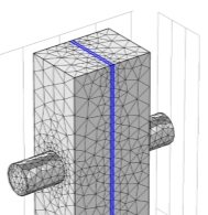
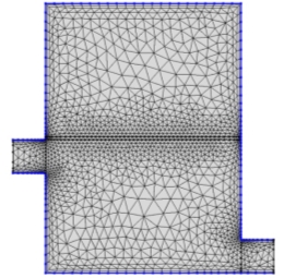
Figure 2.4–User controlled mesh in horizontal and vertical geometry with corner refinements, free triangular and auto adjustment feature activated to improve accuracy of results by non-structured meshing as shown

 

5. Boundary Conditions and dimensions
   1.    Dimensions

For vertical module, dimension of the channel is 2 mm* 3 mm* 30 mm, Inlet and outlet diameter are kept same as 0.75 mm (radius)* 2 mm as in Figure 2.2. Membrane thickness is varied in a range of 150 to 450 µm. The CAD geometry were designed for flat sheet and dead end module. Similarly dimensions for horizontal module were chosen as 3 cm diameter, 2 cm height with permeate tank mounted over feed in Figure 2.3.

2.    Boundary Conditions

The range of experiments are simulated with different initial and final boundary conditions to study the behaviour of the results of the initial run are described in Table 3.1, 3.2 and 3.3. Entrance velocity on feed is varied in range of 1.75 to 5 m/sec on feed side and Exit velocity of permeate side is varied from 1.75 to 2 m/sec on the permeate side. Likewise temperatures are varied within a range from 273 K to 363 K for condenser and heat source. The following methodology is followed for carrying simulation. Step (A)-The temperature of the condenser is fixed and temperature of source is manipulated and (B) The temperature of the heat source is fixed and temperature of condenser is manipulated.

 

3. Results and Discussion
   1. Effect on Dusty gas parameters with laminar and turbulent flow regime assumptions

Sieder Tate equation used for laminar flow condition where high deviation was noticed in [19] whereas Dittus-Boelter equation using equation (9) for turbulent flow condition low deviation was noticed in this study. MATLAB simulation has justified the results. Heat loss due to q_c (heat conduction) is large to q_v (convectional heat transfer) at temperature lower than 325 K as feed side parameters fluctuates much as compared to permeate as shown in Table 3.1 and 3.2 , q_v contributes nearly 92% of the total heat transfer so the other (q_c) can be easily disregarded. Assumed temperature is deviated only ±5% by [5] and majority of mass transfer is taking place in transition zone. The Dusty gas parameter calculated are shown in Table 3.3. Similarly deviation of parameters with respect to each other are shown in Figure 3.1 to Figure 3.15.

Table 3.1 –Permeate side simulation results showing Nusselt no. is very small

Rho	Dynamic Viscosity (x10-5)	Specific heat	Conductivity	Reynolds No.	Prandlt No.	Nusselt No.	Heat transfer coefficient
Kg/ (m3)	Kg/m.sec	J/kg.K	Watt/m.K				Watt/m.K
999.192488	99.2	4179.922303	0.605300	21153.536870	6.849880	0	471717683.073985
999.192492	99.2	4179.922302	0.605300	21153.531567	6.849882	0	471717618.260156
999.192496	99.2	4179.922301	0.605300	21153.527510	6.849883	0	471717568.667171
999.192498	99.2	4179.922300	0.605300	21153.524313	6.849885	0	471717529.592130

 

Table 3.2 –Feed side simulation results

Rho	Dynamic Viscosity (x10-5)	Specific heat	Conductivity	Reynolds No.	Prandlt No.	Nusselt No.	Heat transfer coefficient
Kg/ (m3)	Kg/m.sec	J/kg.K	Watt/m.K				Watt/m.K
984.054758	45.8	4183.976408	0.673470	45141.110337	2.844051	0	718013358.162020
987.678756	54.1	4183.005848	0.657150	38313.587600	3.445928	0	655077781.376065
991.642504	65.8	4181.944299	0.639300	31647.212870	4.304399	0	589008146.611555
995.455252	80.4	4180.923190	0.622130	25997.373995	5.403842	0	528327223.714031

 

 

 

 

 

Table 3.3 –Dusty gas model parameters

Dk	Ppm	Pfm	Pap	Paf	N	Flux
m2/sec	Pascal	Pascal	Pascal	Pascal	Kg/m2.sec	Kg/m2.hr
0.000045	2321.806503	20046.737027	99003.193497	81278.262973	0.007767	27.959645
0.000044	2321.803128	12660.687813	99003.196872	88664.312187	0.004381	15.770343
0.000044	2321.800547	7375.429498	99003.199453	93949.570502	0.002083	7.500329
0.000043	2321.798512	4207.525405	99003.201488	97117.474595	0.000762	2.741919

2. Effect of surface energy, thermal conductivity and porosity on performance

Reasonably large pore size and narrow pore size distribution limited by the minimum Liquid Entry Pressure (LEP) of the membrane restricts membrane fouling [1]. In MD, the hydrostatic pressure must be lower than LEP to avoid membrane wetting. This can be calculated by the Laplace (Cantor)

Liquid Entry Pressure=-2B γRangle cosine< Psystem-Pwith pores

———-12

Where, B is a geometric factor,

γis the surface tension of solution, angle cosine is the contact angle between solution and membrane surface which depends on hydrophobicity of the membrane,

Ris the largest pore size,

Psystemis the liquid pressure on the either side of the membrane and

Pwith poresis the air pressure in the membrane pore.

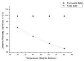
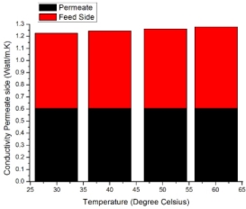
Figure 3.1 –Dynamic Viscosity   Figure 3.2 – Conductivity

 

Using equation (17) we predicted the conductivity of the membrane. Conductivity of membrane is a function of conductivity of vapour present inside membrane, conductivity of liquid present on either side of membrane and porosity (void fraction) of the membrane. Reverse calculation is performed to estimate the indirect effect of LEP in section 3.3, 3.5 and 3.6. Figure 3.1 shows dynamic viscosity decreasing linearly with increase in temperature. As dynamic viscosity decreases thermal boundary layer dominates over hydrodynamic boundary layer with decrease in Prandlt number and increase in conductivity as shown in Figure 3.2.

3.3 Effect of TPC on temperature contours along the cross section and effect of temperature gradient on membrane interface temperature

To justify the results a script was run in MATLAB.  Dusty gas equations were used to study the process, input for the values of

Tfm,

Tf,

Tpm and Tpvalues as mentioned in Table 3.4 were taken by user. Number of iteration were counted and noted down to keep a record of steps taken to attain a steady value of temperature at interface. Interface temperatures calculated were responsible for best mass flux values after convergence is achieved. The same has been validated qualitatively through computational fluid dynamics simulations.

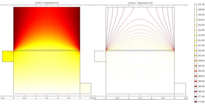
TPC decreases significantly with decrease in the operating temperature for permeate as shown in Figure 3.3, it should be slightly lower than or equal to thermal efficiency (η) 0.5. TPC value varies from 0.61 to 0.77. Surface temperature of the TPC plot explained based on the results in [12].Results are highly in accordance with reported resultby Besagni et al. [23]. Shorter modules are less vulnerable to TP effects and have higher TPC than longer modules [13].

TPC decreases significantly with increase in H (mass transfer coefficient) as reported in [9] by Yu et al. lower the H decreases, mass flux showed an increasing trend. At lower H value DCMD module was found to be less susceptible and prone to polarization effects.

Figure 3.3 –Temperature polarisation effects which are qualitatively described above with surface temperature and contour lines on feed (boiler) and permeate (condenser) sections with legend bar showing range

TPC is the indirect coefficient used to evaluate the boundary layer resistances for well-designed MD, TPC approaches unity [6] using equation (13) showed agreement with surveyed literature.

Table 3.4- T_fm and T_pm are found by Monte Carlo Simulation and optimized using iterations making comparison of other decisive parameters

| Tfb	Tfm	Tpb	Tpm	No. of Iterations	Tfm after interations	Tpm after interations
Degree Celsius	Degree Celsius	Degree Celsius	Degree Celsius		Degree Celsius	Degree Celsius
60.10	59.00	10.00	21.00	2	40.001	20.006
50.50	49.00	15.00	21.00	4	39.90	20.005
40.00	39.00	17.00	21.00	6	39.89	20.005
29.90	28.00	18.00	21.00	8	39.88	20.003

TPC=Tfm-TpmTf-Tp=11+Hh=1-Hh

———-13

The feed and permeate TPC are defined as-

TPC= TPCp+TPCf-1 ———–14

4. Effect on performance due to dimensionless quantity (Reynolds number)

Experiments were conducted for horizontal module as shown in Figure 2.3. partial pressure increases with increase in Reynolds number, the simulation was performed at ten different values of Reynolds number (based on the Inlet and Outlet diameter) ranging from 3300 to 7000 with the inlet feed velocities from 1m/sec to 5.75m/sec. Saline water flows at 60^oC through the inlet feed from lower end and permeate cold water is fed at 20^oC from upper end as shown in Figure 2.2. The rejection of salt from solution is more than 95% which is predicted by the conductivity of the permeate fluid. Here Prandlt number is near to value of 7 in Table 3.1 on the permeate side as described by Matsuura et. al in [17] and decreases on feed side with increase temperature which says about the viscosity and conductivity shown in Figure 3.5.

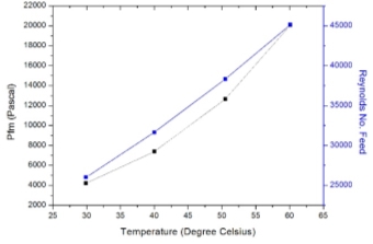
Figure 3.4 –Feed interface temperature with membrane, Reynolds number with respect to input temperatures

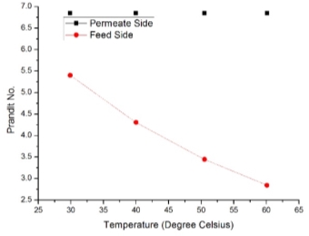
Figure 3.5 –Prandlt number variation on permeate and feed side with respect to temperature

 

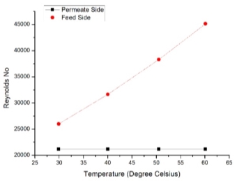
Figure 3.6 – Reynolds number variation on permeate and feed side with respect to temperature

 

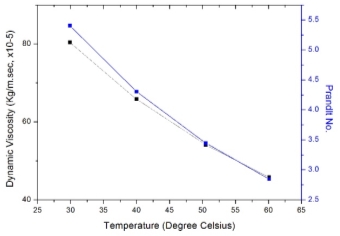
Figure 3.7–Dynamic viscosity falls almost at a similar rate as Prandlt no.

 

5. Pressure Contours at various locations and pressure drop

Partial and vapour pressure were evaluated using numerical methods, data has been calculated and plotted along the length of the module for different temperature values ranging from 273 K to 333K. Equation (15) was used for calculation of diffusion (D_k) with help of antoine’s equation where A= 23.238, B=3841 and D=-45 and equation (15) Water vapour pressure on permeate membrane interface was

Ppm=eA-BTpm+Dand feed membrane interface was

Pfm=eA-BTfm+D

Then

papand

pafwere calculated using,

pap=101325-Ppmand

paf=101325-Pfm

P×Dk=4.46106×T2.334

———-15

The values of pressure variations along the feed-membrane interface shown in Figure 3.9 shows that vapour pressure variation increases with increase in temperature which helps in better mass flux across the membrane. Streamline graphs helped in rectifying very crucial design modification to improve hydrodynamics as shown in Figure 3.8.

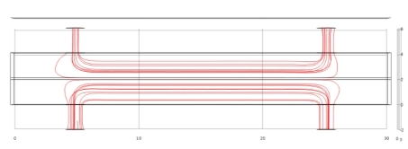
Figure 3.8–Streamline depicting irregularities in fluid dynamics which can mitigated by improvement in module design.

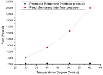
Figure 3.9–Partial pressures on feed and permeate side

 

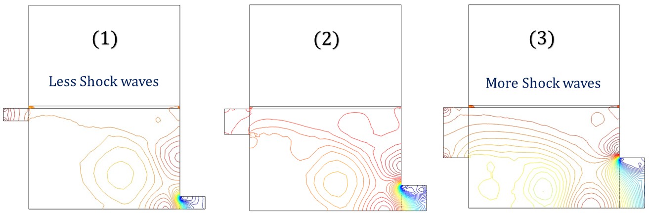
Figure 3.10 (a)

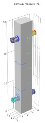
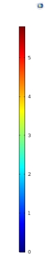
Figure 3.10 (b)

Figure 3.10– Pressure contours for (a) horizontal and (b) vertical profile, the legend bar depicts pressure in Pascal’s.
 

6. Effect of the module length or diameter on flux and heat transfer coefficients

In shorter modules, where thermal Boundary layer are still developing at the exit

∆Tfcurves are of similar shapes as

∆Tpalong the flow direction. Whereas, in longer modules, thermal Boundary layer is fully developed [1], [25].

The magnitude of q_pis larger than q_f because the permeate side has smaller contact area (inner membrane wall) than the feed side (outer membrane wall), with a local heat transfer rate (flux) imposed at the same location in the radial direction, q_pis larger than q_f.. For flux calculation primary consideration is value of Knudsen number defined as,

Kn=λD

where,

λ= 0.11

×10-6m is used as mean free path and

D = 0.22

×10-6 m is used as pore diameter, value of

Kncomes as 0.5 it shows Knudsen number lies between lies between 0.01<

Kn<1, so we can evaluate flux using Knudsen- molecular diffusion transition

N =

εMτδRT1Dk+PaPfDkln-1ln(Pfm -Ppm) ———-16. So Q can be calculated to evaluate

ηby equation

, η=Qq+Q. When Knudsen diffusion is calculated, Poiseulli’s equation is also evaluated. Both were added to calculate total flux Q. Calculation of heat transfer coefficients on both feed and permeate side was done by putting Q from above result and

ηas unknown. Validation between results obtained by numerical methods and parameters calculated by Dittus Boelter equation as shown in Figure 3.11 had proved permeate heat transfer coefficient were more stable than on feed side. Similarly, an analogy can be established between heat and mass transfer phenomenon. It predicts heat transfer coefficients were dependent on inlet velocity and feed temperature as shown in figure 3.12.

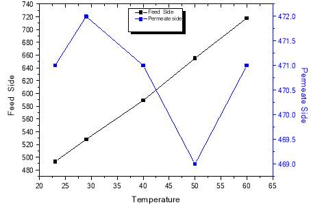
Figure 3.11 –Feed and permeate side heat transfer coefficients.

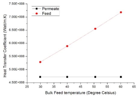
Figure 3.12 –Feed and permeate side heat transfer coefficients.

 

To investigate response of characteristics length with respect to Nusselt number it was observed that shorter modules tend to have relatively higher Nu_{p .}and Nu_f   then the longer one. Nu_psubscript p denotes permeate side and f denotes feed side. Nu_f   increases with increase in Re_f reported in [6].

The equation for thermal conductivity used is

km=1-ϵkg+ϵkp—— (17) and the heat transfer coefficients calculated from

hm=kmδ  , heat transfer coefficient multiplied with thickness of membrane gives conductivity as discussed in section 3.2. Likewise on calculation it was found that dimensions used for module in creating simulations of membrane distillation are satisfactory. Figure 3.13, heat transfer coefficient effecting flux with different module dimensions, 15 mm module length is found to be better than 5, 30 and 45 mm.

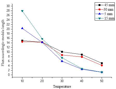
Figure 3.13–Flux according to different module length shows similar results as in [1] by Tzahi  et al. and the one with 15 mm length is better

7. Varying flow distributions and change in velocity profile with arc length

The dimension of the module length has effects on velocity and pressure drop. Operating the module at higher feed and permeate circulation velocities increases the trans-membrane flux but thermal efficiency decreases due to greater heat loss. A thorough consideration of the heat transfer parameters (q, TPC, N_uand η) was conducted. Figure 3.15(a) shows velocity drop along inlet and outlet of different dimension on the feed and permeate side of MD module. Membrane properties, module configurations and system energy recovery is essential for meeting the expected outcome. The results shown in Figure 3.14(b) shows difference in drop velocities due to change in module dimensions and temperature when coupled with different mass flow velocities. Curl shown in second geometry in Figure 3.14 (a) shows proper distribution than other geometries.

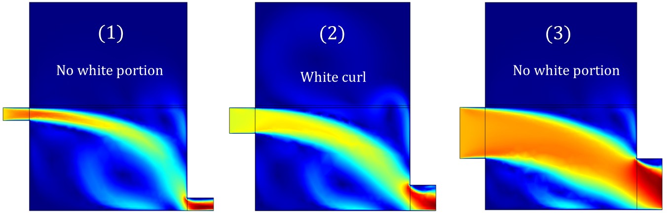
Figure 3.14 (a)

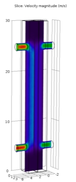
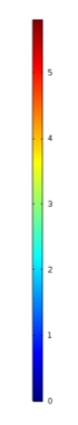
Figure 3.14 (b)

Figure 3.14–Velocity distribution profile for (a) horizontal and (b) vertical profile, the legend bar depicts velocity 0 m/sec to 5.75 m/sec. The red portion is at high velocities leading describing drop in velocity and pressure

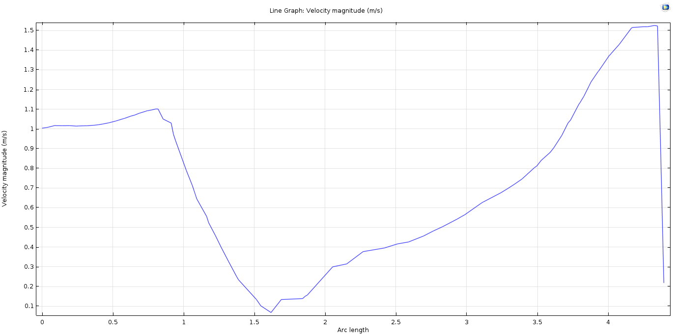
Figure 3.15–The above result plotted between two points along the arc length within a horizontal module shows high fluctuations in velocities which should be mitigated by optimizing the design

8. Comparison of experimental and predicted flux using Monte Carlo Simulation

In [13], Yu et Al. used Monte Carlo procedure to study efficiency related to heat flux Q as,

η=Qq+Q. Here

Qvapour heat flux and q is condensed water heat flux. Total heat flux can be written as a function of mass flux as mentioned in [16] and [22]. The heat transfer coefficients on the shell side was nearly half then on the lumen side. Shell side heat transfer hydrodynamics played important role in improving MD configuration as shown in section 3.8. At steady state, heat balance equation utilises calculated parameters to evaluate

Tfmand

Tpmusing following equation

Tfm=hpTp+hfhpTf+hfTf-N∆Hvhp+hf1+hmhp—–18 and likewise

Tpmis also calculated. In Table 2.1 based on the input parameters described in section 2.1 optimized value of interface temperature is shown.

Table 3.5 shows comparison of results from experimental data taken from [9], [1] andpredicted flux value. So a new membrane cell was designed to hold a flat-sheet membrane under moderate pressure gradients without a physical support. Design consideration included maximizing mixing and minimising of pressure drop in flow channels. By optimizing channel cross section, length and smoothness better performance can be achieved. Minimization of heat loss to the surroundings by using acrylic plastic is observed. Results in Table 3.5 were plotted to show deviations from experiments [1] shown in Figure 3.16.

Table 3.5-Depicting the predicted flux values from simulation/coding and expected flux values from published paper, titled as “Experimental study of desalination using direct contact membrane distillation: a new approach to flux enhancement” authored by Tzahi Y Cath, V Dean Adams, Amy E Childress and Journal of membrane science 228 (2004) 5-16.

SL No.	Feed Temperature (oC)	Predicted Flux (Pi), (Kg/m2.hr)	Experimental Flux (Ei), ( (Kg/m2.hr)
1	60.1	27.95	27.4
2	50.5	15.77	17.0
3	40.0	7.5	11.0
4	29.9	2.74	3.6

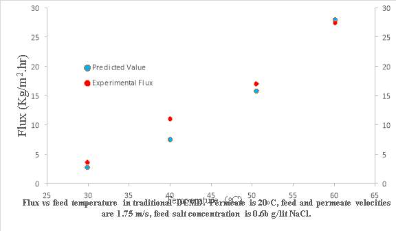
Figure 3.16–Predicted flux and experimental flux plotted against temperature

1.      Error Analysis

Here RMSE is root mean square error which was used to calculate RE (Relative Error), where

Piis predicted or model value,

EiExperimental value,

E̅mean of the experimental value and n number of points analysed using relation

RMSE=∑i=1n(Pi-Ei)2n

———19

RE=RMSEE̅

———20

2.      Willmott Index (d)

Finally, d was calculated as Willmott index using the following relationship. Modeling was done based on the criteria mentioned in Table 3.16. Figure 3.16 justifies the accuracy of predicted data graphically.

d=∑i=1n(Pi-Ei)2∑i=1n{Pi-E̅+|Ei-E̅|}2

———21

Criteria Range	Model Type
d => 0.95 and RE =< 0.10	Model is Very Good
d => 0.95 and RE =< 0.10	Model is Very Good
d => 0.95 and 0.10 <= RE <= 0.15	Model is Good
d => 0.95 and 0.15 <= RE <= 0.20	Model is Marginal
d => 0.95 and 0.20 <= RE <= 0.25	Model is Poor

Table 3.6– Willmott Index criteria list shows d and RE lies between 0.95 and 0.10 to 0.15.

 

The Willmott index, d is 0.9889 and value RE (Relative error) is 0.1304 which is good and is within acceptable range.

3.      Convergence

Repeatability and reproducibility of the phenomenon was achieved with low level of errors which comes to be in the order of three decimal places. The numerical simulation converges in 5 minutes giving suitable results within validation range.

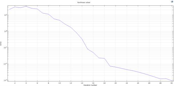
Figure 3.17–Error percentage and the accuracy lies within three decimal places and convergence attained shows repeatability and reproducibility.

 

4. Conclusion

In this study, we analysed in detail the variation of flux with respect to channel length of feed and permeate, pressure contours, temperature profile, velocity distribution, relative error in convergence of numerical results and Willmott index. CFD simulation have been performed systematically in COMSOL version 5.2 for the purpose of achieving optimized temperatures and pressure. The results obtained through computational fluid simulations were extracted and used to obtain suitable design parameters and helped in suggesting appropriate manipulations. The assumptions that were used to converge the results were, negligible inertial terms, no radial dependence or axial pressure profile, Newtonian behaviour, symmetry boundary condition. The Dirac function is taken into account to assume uniform membrane network of uniform pores considered as roughly about over 5000 and result is averaged over 30 readings and validated using Monte Carlo simulation.  From the analysis, following conclusions can be drawn.

1. To minimise the heat loss in the membrane, higher feed temperature and lower thermal conductivity is required. High thermal conductivities increases sensible heat transfer and reduce vapour flux.
2. High porosity increases both thermal restrictions and permeability, as a result both the efficiency and flux were increased. On the contrary, high porosity tend to crack membrane. Low surface energy is indication of high hydrophobicity.
3. Present work showed evaluation of Willmott index (d) as 0.9889 and Relative Error (RE) as 0.1304. Flux obtained was 27 kg/m2.hr at 60^oC with a dimension of 15 mm length, 2 mm width and 3 mm depth of the channel for feed and permeate each.
4. TPC is decreased and N_u is increased with higher operating temperatures. Thermal efficiency is also improved since temperature polarization coefficient is inversely proportional to the thermal conductivity.
5. Tortuosity (

   τ) is reciprocal of porosity, In MATLAB, script porosity has been put with a fixed value of 0.7 so reciprocal of porosity comes as 1.47 to 1.54.

6. Using a correction factor in Dittus- Boelter equation as ,

   1+6DiameterLpthe heat transfer coefficient calculated was more precise and realistic

7. Polarization effects indirectly quantifies the boundary layer resistances for well-designed MD. Concentration polarization is less effective when compared to temperature polarization.
8. Prandlt Number decreases to increase thermal boundary layer thickness on feed side. TPC tends to approach unity. h becomes high enough so that the whole term

   Hhterm can be neglected with H tending towards zero.

9. Temperature effects are more pronounced and realistic when viscous flow in taken into consideration. A deviation from Knudsen diffusion) is experienced when viscous heat is included in simulation.The model was verified using results from system identification toolbox.
10. Moving reference frame methodology using computational methods when applied with symmetric boundary condition were simulated to show better permeability. With accurate temperature and fluid mechanics coupling, permeate and feed heat transfer coefficients are evaluated. Flux was found to be increasing with higher stirrer speed to decrease the TPC effects.
11. MD can work at low operating temperature, pressure and low thermal energy requirement but thermal efficiency is much lower. DCMD can be made economical in applications which can utilise recovered waste heat to purify saline water. Water purification in Middle East is satisfying almost 55% of its total consumption using these techniques.
12. Monte Carlo (MC) simulation random inputs between a range of 1 m/sec and 5.75 m/sec were taken to study the porosity and tortuosity.  Membrane permeability prediction is been carried out using MC simulation. Heat flux and enthalpy calculation are evaluated using empirical relation-

    HvT=1850.7+2.8273T-1.6 X 10-3T2and optimum value was reported.

NOMENCLATURE

Greek Letters

μ

viscosity

ρ

density

δT

chosen grid thickness in grid r direction

τ̿

stress tensor

η

energy efficiency

τ

tortuosity

ε

porosity or void fraction

Subscripts

fm feed-side membrane surface

pm permeate-side membrane surface

p  permeate

f feed

J_i Flux at generic point

P₁ Initial pressure

P₂ Final pressure

v⃗

velocity vector in generic direction

k conductivity

T_fm temperature on feed membrane interface/surface

T_pm temperature on permeate membrane interface/surface

T_f temperature of bulk feed

T_p temperature of bulk permeate

P_ap partial pressure on permeate side

P_fm vapour pressure on feed membrane interface/surface

P_pm vapour pressure on permeate membrane interface/surface

P_af partial pressure on feed side

H overall heat transfer coefficient

L characteristic length

R_m membrane resistance

d hydraulic diameter or length of the pore

REFERENCES

[1] T. Y. Cath, V. D. Adams, A. E. Childress Experimental study of desalination using direct contact membrane distillation: A new approach to flux enhancement. Journal of Membrane Science 228 (1) (2004) 5–16.

[2] C. P. Om Ariara Guhan, G. Arthanareeswaran, K. N.Varadarajan, S. Krishnan, Numerical optimization of flow uniformity inside an under body- oval substrate to improve emissions of IC engines. Journal of Computational Design and Engineering 3(3) (2016) 198–214

[3] C. P. Om Ariara Guhan, G. Arthanareeswaran, K. N. Varadarajan. CFD Study on Pressure Drop and Uniformity Index of Three Cylinder LCV Exhaust System. Procedia Engineering 127 (2015) 1211–1218.

[4] A. Burgoyne, M. M. Vahdati, Direct Contact Membrane Distillation. Separation Science and Technology 35(8) (2000) 1257–1284.

[5] M. Khayet, Membranes and theoretical modeling of membrane distillation: A review. Advances in Colloid and Interface Science, 164(1–2) (2011) 56–88.

[6] H. J. Hwang, K. He, S. Gray, J. Zhang, I.S. Moon, Direct contact membrane distillation (DCMD): Experimental study on the commercial PTFE membrane and modeling. Journal of Membrane Science, 371(1–2) (2011) 90–98.

[7] J. Phattaranawik, R. Jiraratananon , A. Fane, Heat transport and membrane distillation coefficients in direct contact membrane distillation. Journal of Membrane Science, 212 (1) (2003) 177–193.

[8] R.W. Schofield, A.G. Fane, C.D.J. Fell, Gas and vapor transport through microporous

Membrane. II. Membrane distillation, J. Membr. Sci. 53 (1990) 173.

[9]  H.Yu, X. Yang, R. Wang, A. G. Fane, Analysis of heat and mass transfer by CFD for performance enhancement in direct contact membrane distillation. Journal of Membrane Science, 405–406 (2012) 38–47.

[10] V. A. Bui, L. T. T. Vu, M. H. Nguyen, Simulation and optimisation of direct contact membrane distillation for energy efficiency. Desalination, 259 (1–3) (2010) 29–37.

[11] J. Phattaranawik, R. Jiraratananon, Direct contact membrane distillation: Effect of mass transfer on heat transfer. Journal of Membrane Science 188 (1) (2001) 137–143.

[12] A. Burgoyne, M. M. Vahdati, Direct Contact Membrane Distillation. Separation Science and Technology, 35(8) (2000) 1257–1284

[13] M. Khayet, A. O. Imdakm, T. Matsuura, Monte Carlo simulation and experimental heat and mass transfer in direct contact membrane distillation. International Journal of Heat and Mass Transfer 53(7–8) (2010) 1249–1259.

[14] A. O. Imdakm, T. Matsuura, A Monte Carlo simulation model for membrane distillation processes: Direct contact (MD). Journal of Membrane Science 237(1–2), (2004) 51–59.

[15] V. A. Bui, L. T. T. Vu, M. H. Nguyen, Modelling the simultaneous heat and mass transfer of direct contact membrane distillation in hollow fibre modules. Journal of Membrane Science 353(1–2) (2010) 85–93.

[16] H. Yu, X. Yang, R. Wang, A.G. Fane, Numerical simulation of heat and mass transfer in direct membrane distillation in a hollow fiber module with laminar flow. Journal of Membrane Science 384(1–2) (2011) 107–116.

[17] M. M. M. Su, K.Y. Teoh, T. S. Chung Wang, Effect of inner-layer thermal conductivity on flux enhancement of dual-layer hollow fiber membranes in direct contact membrane distillation. Journal of Membrane Science, 364(1–2) (2010) 278–289

[18] G. Chen, X. Yang, R. Wang, A. G. Fane, Performance enhancement and scaling control with gas bubbling in direct contact membrane distillation. Desalination, 308 (2013) 47–55.

[19] J. Gilron, , L. Song, K. K. Sirkar, Design for cascade of crossflow direct contact membrane distillation. Industrial and Engineering Chemistry Research, 46(8) (2007) 2324–2334.

[20] A. M. Alklaibi, N. Lior, Comparative study of direct-contact and air-gap membrane distillation processes. Industrial and Engineering Chemistry Research, 46(2) (2007) 584–590.

[21] D. Singh, K. K. Sirkar, Desalination of brine and produced water by direct contact membrane distillation at high temperatures and pressures. Journal of Membrane Science 389 (2012) 380–388.

[22] A. O. Imdakm, T. Matsuura, Simulation of heat and mass transfer in direct contact membrane distillation (MD): The effect of membrane physical properties. Journal of Membrane Science 262(1–2) (2005) 117–128.

[23] G. Besagni, R. Mereu, F. Inzoli, P. Chiesa, Application of an Integrated Lumped Parameter-CFD approach to evaluate the ejector-driven anode recirculation in a PEM fuel cell system. Applied Thermal Engineering (2017)

[24] R. Al-waked, M. S. Nasif, G. Morrison, M. Behnia, CFD simulation of Air to Air Enthalpy Heat Exchanger: Variable Membrane Moisture Resistance. Applied Thermal Engineering (2015)

[25] I. Hitsov, T. Maere, K. De Sitter, C. Dotremont, I. Nopens, Modelling approaches in membrane distillation: A critical review. Separation and Purification Technology 142 (2015) 48–64.

[26] J. Woods, E. Kozubal, Heat transfer and pressure drop in spacer-filled channels for membrane energy recovery ventilators. Applied Thermal Engineering 50 (1) (2013) 868–876.

[27] L. Sikos, J. Klemeš, J. Reliability, Availability and maintenance optimisation of heat exchanger networks. Applied Thermal Engineering 30 (1) (2010) 63–69.

[28] S. Wright, G. Andrews, H. Sabir, A review of heat exchanger fouling in the context of aircraft air-conditioning systems, and the potential for electrostatic filtering. Applied Thermal Engineering 29 (13) (2009) 2596–2609.

[29] H. Yu, X. Yang, R. Wang, A. G. Fane, Analysis of heat and mass transfer by CFD for performance enhancement in direct contact membrane distillation. Journal of Membrane Science 405–406 (2012) 38–47.

[30] H. Yu, X. Yang, R. Wang, A. G. Fane,  Numerical simulation of heat and mass 30transfer in direct membrane distillation in a hollow fiber module with laminar flow. Journal of Membrane Science 384(1–2) (2011).  107–116.

[31] X. Yang, H. Yu, R. Wang, A. G. Fane, Optimization of microstructured hollow fiber design for membrane distillation applications using CFD modeling. Journal of Membrane Science 421–422 (2012) 258–270.

[32] M. M. A. Shirazi, A. Kargari, A. F. Ismail, T.  Matsuura. Computational Fluid Dynamic (CFD) opportunities applied to the membrane distillation process: State-of-the-art and perspectives. Desalination 377 (2016).  73–90.

[33] C.D. Ho, H. Chang, C.H. Tsai, P.H. Lin, Theoretical and Experimental Studies of a Compact Multiunit Direct Contact Membrane Distillation Module. Industrial & Engineering Chemistry Research 55(18) (2016) 5385–5394.