Flood Modelling and Forecasting Methods and Management Strategies
Info: 5876 words (24 pages) Dissertation
Published: 12th Dec 2019
Table of Content
Task A – Estimation of 1% AEP flood
Task B – Flood Forecasting, Warning and Control
Reduction of operational costs
Task A – Estimation of 1% AEP flood
Catchment´s characteristics
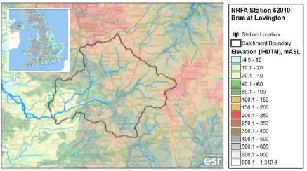 The Brue at Lovington catchment is located at the south of the UK (Fig. 1) and has an area of 135.2 km2. It is fed upstream by Mendip and Salisbury Plain springs. The geology goes from Oxford Clay and Great Oolite in the upper part to Yeovil Sands and Inferior Oolite in the lower-catchment (CEH, 2018).
Figure 1: Location of the Brue at Lovington catchment. Source: CEH (2018)
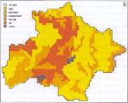 The land use is mainly rural with little urbanization. In 1983, after flooding events in the town (1968, 1979 and 1982), the Burton Dam reservoir was constructed, it drains 21% of the catchment (CEH, 2018). The FARL index is 0.997 which means there is almost no flood attenuation due to reservoirs or lakes. The percentage of runoff derived using the hydrology of soil types classification is low (Fig. 2), meaning it’s moderately impermeable (SPRHOST = 36.27; Shaw et al., 2014).
Figure 2: Classification of soil types in the Brue catchment. Source: Mellor et al. (2000)
The Station is located west of Lovington, opened in 1964 and rebuilt in 1998. For the period record of 1964 to 2016 the mean flow recorded was of 1.938 m3s-1. The summer weed growth downstream affects the stability of the stage-discharge relationship (CEH, 2018).
In the catchment, some flood management plans have been made, one is the North and Mid Somerset Catchment Flood Management Plan to assess inland flood risk across all of England and Wales. The other is the South Drain Water Level Management Plan for the Lower and Upper Brue Drainage Board.
FEH WINFAP statistical method
There are different statistical distributions that can be used to represent flood peak frequencies, a software package that’s used is WINFAP – it was produced as part of the Flood Estimation Handbook (FEH; Shaw et al., 2014). It’s a statistical method that uses observations of flow or river gages directly in a frequency analysis. This approach estimates the peak flow for a given return period, in this case for 100 years, consists of the following steps: the estimation of the index flood (median annual maximum flood – QMED), the estimation of an appropriate flood growth curve, and the derivation of a flood frequency curve which relates the index flood to the growth curve – providing an estimate of the peak flow for the return interval (Wallingford HydroSolutions Ltd, 2009). Both a Single Site and Pooled Analysis of flood-peak data were carried on for the period of 1964-2007. A time series graph was also made, the flow peak record was of 141.568 m3s-1 for May 30, 1979.
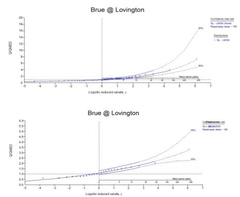 The Single Site Analysis is based on an observed flood series at the catchment and cannot be applied to ungauged catchments (Wallingford HydroSolutions Ltd, 2009). A General Logistic distribution was applied with the L-Moments technique. It was also considered the construction of the dam in 1983, so a second analysis considered only from this point was done. Growth curves, with 95% confidence limits were obtained (Fig. 3). This growth curves normalize the floods observed by dividing the value by the index flood, which is the median annual maximum flood flow (flood that is exceeded on average in exactly half of all years with a 2 years return period); this provides a non-dimensional scale of discharge (Shaw et al., 2014). The annual maximum discharge for a return period of 100 years was 50.376 m3s-1 for the complete period and 77.776 m3s-1 for the period since the dam was constructed.
Figure 3: a) Growth curve with a 95% confidence interval for the period of 1964-2007; b) Growth curve with a 95% confidence interval for the period of 1983-2007.
A Pooled Analysis was also done using the General Logistic distribution. This can be applied to an ungagged catchment as it uses the catchments characteristics to identify a number of gauged catchments that are hydrologically similar to it (Wallingford HydroSolutions Ltd, 2009). To select the pooling stations the BFIHOST (Baseflow Index) was considered, as it is the fraction of the total hydrograph that is derived from baseflows and has to be similar between the stations (Wallingford HydroSolutions Ltd, 2009). The group was strongly heterogeneous. This analysis was done for the entire period as well as just from 1983 (dam construction).
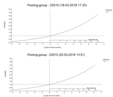 The following growth curves were obtained (Fig. 4):
Figure 4: a) Growth curve for the period of 1964-2007; b) Growth curve for the period of 1983-2007.
FEH Rainfall-Runoff method
The FEH ‘revitalized’ flood hydrograph method was used. This model consists of: a loss model converting total rainfall into effective rainfall, a routing model, and a baseflow model (Kjeldsen, 2007).
In this model, the seasonal design rainfall depth is obtained by the multiplication of the RDDF (point estimate of design rainfall obtained from the FEH DDF model), the ARF (areal reduction factor transforming point rainfall to catchment average rainfall), and SCF (seasonal correction factor transforming annual maximum rainfall to seasonal maximum rainfall; Kjeldsen, 2007).

The time to peak can be estimated from catchments descriptor as shown below, and then from the Tp the duration time can be obtained:


The temporal distribution of the rainfall-runoff process is modelled using a design storm profile. The revitalized method adopted a 75% winter profile (Kjeldsen, 2007).
To obtain the 100-year design flood event it’s estimated from the input design rainfall event and the soil moisture content. The loss model is applied and it estimates the fraction of the total rainfall volume turned into the direct runoff (Kjeldsen, 2007). Then this direct runoff is routed to the catchment outlet using the unit hydrograph convolution, using a ‘kinked triangle’ unit hydrograph, to finally add the baseflow and obtain the total runoff (see Annex 3; Kjeldsen, 2007).
The following design flood hydrograph was obtained (Fig. 5), the peak flow was equal to 121 m3s-1.
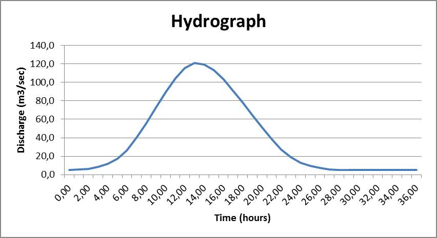
Figure 5: Design flood hydrograph.
SHETRAN simulation method
The continuous simulation converts rainfall time series from a stochastic rainfall model into a hydrograph using a catchment rainfall-runoff model. SHETRAN is a coupled surface/subsurface physically based spatially distributed 3D finite difference model that allows to model the flow and transport of a basin (Ewen et al., 2000). It is based on the hydrological modelling system SHE (Systéme Hydrologique Europeèn) which considers interception, evapotranspiration, snowmelt, overland and channel flow, unsaturated and saturated zone flow for the water movement through the river basin (Mellor et al., 2000).
The output given was evaluated on WINFAP obtaining the following time series graph, the peak flow for the catchment was of 92.542 m3s-1. A Single Site Analysis was done following the same criteria as used for the FEH statistical method (Fig. 6).
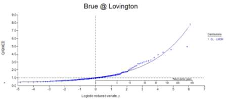
Figure 6: Growth curve for the 200 year period.
In addition, a Gumbel plot was done, where the magnitude of the event vs. the rarity or frequency on a reduced variate scale is graphed. On Fig. 7 the growth curve standardized by the mean is displayed.
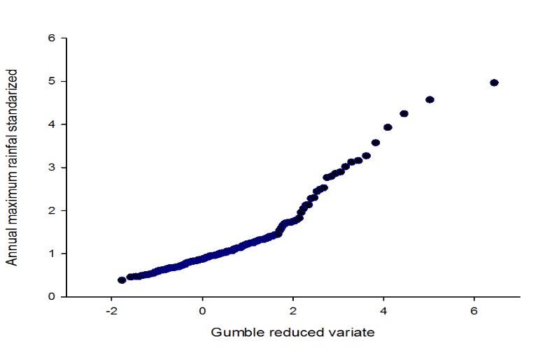
Figure7: Growth curve standardized by the mean.
Comparison of methods
Flood frequency analysis were done, by the application of different methods, with the aim of estimating the peak discharge which is likely to be equaled or exceeded on average once in 100 years. On Table 1 the results obtained are showed. The runoff values for the 100 year peak flow obtained are plausible, having in consideration that the catchment is relatively permeable with little urbanization.
Table 1: Table of comparison between the results of the different methods used in this coursework.
| Method | 100 year return period (m3s-1) | Period | Number of readings |
| FEH WINFAP statistical method-Single site | 150.376 | 1964-2007 | 44 |
| FEH WINFAP statistical method-Single site | 77.776 | 1983-2007 | 25 |
| FEH WINFAP statistical method-Pooled analysis | 111.049 | 1964-2007 | 518 |
| FEH WINFAP statistical method-Pooled analysis | 89.749 | 1983-2007 | 502 |
| FEH Rainfall-Runoff method | 121 | – | – |
| SHETRAN simulation method-WINFAP | 92.542 | – | 200 |
The WINFAP statistical and Rainfall-Runoff method are both developed by the FEH to estimate floods. These methods are appropriate for the catchment as it is larger than the recommended limit of 0.5 km2 and it is mainly rural (Shaw et al., 2014). The first one consists of fitting probability distributions to river flow data, while the other one models the rainfall-runoff using design events. One advantage is that they both can be applied for catchments that have flow data or with ungauged locations. This is important as many times sites don’t count with long-term stream gauges (Shaw et al., 2014). On the other hand, these models rely heavily on statistical methods of regionalization of the discharge frequency characteristics against catchment descriptor variables, which can produce uncertain estimates (Shaw et al., 2014).
For the WINFAP statistical method there were only 44 years of data that could be used. This is a problem as to have a reliable estimate we need at least 500 datasets, therefore it’s a limitation. To solve this problem a pooled analysis was done to improve confidence in the estimate, now we were able to count with 518 datasets. This explains the high value of cumecs we obtained for the 100 years return period in the Single site analysis (150.376 m3s-1) in comparison with the rest of the methods. Secondly, it has to be considered the construction of the dam in 1983. If we split the period at this point we see that the first 19 years make a big difference in the results obtained. For the Single site analysis the 100 year return flow goes from 150 to 77 m3s-1, decreasing almost half its value. The Pooled analysis also changes, going from 111 to 89 m3s-1. In conclusion, the best analysis for WINFAP is the Pooled group that takes into account the construction of the dam. As an extra advantage, by WINFAP we could obtain growth curves, that as they have a non-dimensional scale, they can be useful to compare catchments because the form of the frequency distribution doesn’t change (Shaw et al., 2014). Last, both for WINFAP statistical and SHETRAN simulation method peak flows are used, this data is easy to acquire. The only problem is that there might have some uncertainty as rating curves need to be extrapolated beyond the range for which measurements are available (Shaw et al., 2014).
One of the advantages of the FEH Rainfall-Runoff method is that it uses a unit hydrograph rather than peak flows to calculate the volume of the 100 year peak discharge. Also, it allows for estimates to be made for any catchment, even in the absence of observations, which, on the other hand, can be considered as a disadvantage as many arbitrary assumptions and simplifications are made. Last, it is considered a flexible method as many different scenarios can be tested. In spite of this, it is complex and based on single event analysis, which means that antecedent catchment wetness is crucial to estimate losses. In this method, 121 m3s-1 were obtained for the 100 year return period.
One benefit of the SHETRAN simulation model is that surface and subsurface flow are coupled in a simple and direct way (Ewen et al., 2000). As well as being useful for the study of surface and groundwater resources, management and flood control, it can also account the influence of climate change (Ewen et al., 2000; O’Connell, 2018a). The model also handles antecedent conditions automatically, which is a pro, although a good quality and long length of rainfall and flow records is needed for calibration. Some disadvantages are that this method demands great computational work and is still under development.
In my opinion, the FEH WINFAP statistical method with the pooled analysis, considering the dam construction, is the one that gives the most consistent result. Real data from the station on the catchment is used and nearby stations are incorporated to have a more reliable peak flow for the 100 years return period. To improve it, the pooling group could be rechecked in order to make it less heterogeneous.
Alternative strategies
There are some alternative methods that can be applied for unusual catchments. For lowland catchments a modified unit hydrograph can be used, for small catchments the IH 124, the ADAS 345 or the Rational method, and for heavily urbanized catchments the Wallingford procedure or the Modified Rational (EAAA, 2012).
As well, historical reviews and incorporation of floods before the period of gauged records can give more reliable results. This can supply a wider perspective and add credibility to the analysis. Also, it is possible to extend into palaeoflood investigations which use evidence such as sediment deposits, tree rings and pollen to develop very long-term records of major floods (EAAA, 2012).
Task B – Flood Forecasting, Warning and Control
Introduction
For a good flood management, it is indispensable to improve our decision-making process (Todini, 2008). In water resources management, where climate uncertainty exists, river flow forecastings needs to be done (Tucci, 2003). “Prediction is the probability of the flow occurrence based on the historical flow records”, as defined by Tucci (2003) and it is used to help reduce uncertainty and risk.
The forecasts can be made for a short-term (hours or days of lead time) or long-term (up to nine months); flood forecasting, for flash floods, medium, and large basin floods, are done in short-term (Tucci, 2003). One deterministic approach that can be taken in the Quantitative Precipitation Forecast (QPF).The rainfall is recorded by rain-gauges and for the interval between time t and t+(lead time) it’s predicted (Tucci, 2003). There are two main methods to forecast: by “nowcasting” or by the “traditional” method, done with numerical weather predictions (NWP). In the NWP, first, a diagnosis of the current state of the atmosphere is done and then the forecasting begins. These methods can also be combined with observations (radar, etc.) allowing probabilistic forecasts (Kilsby, 2018).
Hydrologic and flood routing models that are used to forecast. The different types of hydrologic models are: empirical (using mathematical equations without relation to the system’s physics), conceptual (using hydrologic concepts) or a combination of both. Conceptual models have two components, the rainfall-runoff module and the routing module (simulates the flow in rivers and reservoirs). The rainfall-runoff models can be distributed, if they consider the spatial variability of the rainfall, state variables and model parameters, or lumped if not (Tucci, 2003). They are classified as physically-based distributed model of Q(x, y, t), lumped conceptual model of Q(t), distribution function model of Q(t), or lumped input-output (transfer function) model of Q(t). The flood routing models can be hydrological, hydrological/hydraulic, or hydraulic (O’Connell, 2018b).
Later, to monitor, improve and compare the forecast quality the model has to be calibrated, verified, and validated. The verification can be qualitative or quantitative. There are four possible outcomes according to the results: 1) correct negatives, 2) miss, 3) false alarm, and 4) hit. Later the quality of the forecast can be evaluated with indicators as the probability of detection (POD) and false alarm ratio (FAR; O’Connell and O’Donnell, 2018). The POD indicates what fraction of the observed events was correctly forecasted, being sensitive to hits. It goes from 0 to 1, being the optimal score 1. The FAR indicates what fraction of the predicted “yes” events actually did not occur. It ranges from 0 to 1 and the optimal score is 0 (Weeink, 2010).
Although hydrological knowledge is usually associated to deterministic models (hydro-meteorological and hydraulic models), rational decisions should take into account all the uncertainties that are part of the hydrological predictands and their associated probability distributions (Todini, 2008). This means that the aim of forecasting is actually the description of the uncertainty of actual future values of hydrological variables. Therefore improvements should aim at reducing the uncertainty in the decision-making process (predictive uncertainty), rather than looking for a better deterministic model (Todini, 2008).
Predictive uncertainty is “the expression of our assessment of the probability of occurrence of a future (real) event conditional upon all the knowledge available up to the present and the information we were able to acquire through a learning inferential process”, Todini (2008). Flood forecasting systems are just a virtual reality of the future, where uncertainty inevitably exists. Emergency managers should make their decisions considering the probability of occurrence of the different events to avoid, as possible, dramatic consequences (economic losses, casualties, etc.; Todini, 2009).
Following this, now it is introduced the concept of joint probability distribution, the predictand y, and the model forecast ŷ. There’ll always exist a difference between y and ŷ generating a scatter that can be used to estimate the joint probability density (Todini, 2008). This is expressed as:

Where ϑ is the specific value of the parameter set used and xt is the input forcing (Todini, 2008).
This conditional uncertainty is unique for a given model, input forcing, initial and boundary conditions, and a set of parameter values; it does not depend on the model choice. If there are additional uncertainties that may affect the estimated value, they have to be “marginalized” (Todini, 2008). It can now be written as:

Where Yt0 is the set of historical predictand observations, Xt0 is the set of historical covariates, yt is the predictand value of interest, xt is the value of the covariate, ϑ is a given parameter vector, Θ is the ensemble of all possible parameter realizations, f(yt |(ŷt|xt , ϑ)) is the probability density of the predictand value conditional upon the covariate and a set of parameters ϑ, and g(ϑ|Yt0, Xt0 ) is the posterior density of parameters given the historical observations (Todini, 2008).
For a given model there’ll be as many joint probability distributions as parameter sets. Consequently, the probability density for the set of parameters ϑ can be derived by the Bayesian inferential process to marginalize out the conditionality on the parameters. This equation will be the basis for deriving the predictive probability density (Todini, 2008). In practice,sometimes it is impossible to evaluate the predictive uncertainty using the Bayesian inferential approach. Therefore, the best set of parameters for issuing predictions and forecasting can instead be estimated. It is referred to as “conditional upon the parameters” where the parameter values are estimated as expected values, as maximum likelihood, etc. (Todini, 2008). Even it might not be necessary to marginalize the parameters, as the predictive uncertainty distribution for the best parameter set may not differ significantly from the obtained by the marginalization process (O’Connell, 2018a).
To assess the predictive uncertainty, there are different hydrological uncertainty processors that can be used (Hydrological Uncertainty Processor HUP, Bayesian Model Averaging BMA, and Model Conditional Processor MCP). The MCP combines the HUP and the BMA together with the convenient properties of the multivariate Normal distribution, allowing to assess the density of the predictand conditional on all the model forecasts at the same time (Todini, 2009). The steps are 1) calculation of a series of n model forecasts ŷ, 2) rankings of the observed values y and the forecasts ŷ and their assignment to cumulative probabilities, 3) via NQT (Normal Quantile Transform) the observed y and forecasted values ŷ are converted into their corresponding Normal space images η and ̂, and 4) a joint distribution is built (of the predictand normal image η conditional on ̂), which is assumed approximately multivariate Normal:

with mean: and covariance:


The result obtained is fairly general and can be applied to one or more predictands as well as conditioned to several forecasting models (Todini, 2009).
Last, we have to distinguish between the term ‘predictive uncertainty’ and ‘validation uncertainty’. The difference is that validation uncertainty measures how well the model reproduces past reality while predictive uncertainty measures how well the model reproduces future reality. Validation uncertainty is useful to evaluate the performance of a model (O’Connell, 2018a).
To finish, as Professor David Archer taught us we have to keep in mind that “all models are wrong but some are useful” and that “there is no need to ask the question ‘Is the model true?’. If ‘truth’ is to be the ‘whole truth’ the answer must be ‘No’. The only question of interest is ‘Is the model illuminating and useful?” (Hewett, 2018).
Best model threshold
For the first point, having in mind that the real warning threshold is 15 m3s-1 and that above this level flood damage occurs, the Probability of detection or hit rate (POD) and the False alarm ratio (FAR) were calculated; both using Microsoft Excel. First, it was determined if a warning should be emitted or not comparing the observed and forecasted discharges and the real warning threshold for 15 m3s-1.
| Observed | |||
| Forecasted | NW | W | |
| NW | 91 | 16 | |
| W | 4 | 27 | |
The formulas used were the following:


It was obtained a value of 0.628 for the POD and of 0.129 for FAR for the threshold of 15 m3s-1.
To obtain the best model threshold the POD and the FAR values were calculated as a reference, to make the decision, for every threshold value from 1 to 60 m3s-1.Also, a new parameter, the Critical success index (CSI) was added as it takes into account the hits, false alarms and misses, giving a more balanced score. It is sensitive to hits and penalizes both misses and false alarms. It ranges from 0 to 1, being the optimal score 1 (Weeink, 2010). All the calculations were done using Microsoft Excel.

The results obtained indicate that the best model threshold is 13 m3s-1(Fig. 8). The FAR is equal to 0.205 and the POD is 0.721. The CSI is equal to 0.608, this was the higher value obtained in comparison with the other thresholds.
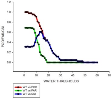
Figure 8: POD, FAR and CSI curves for different water thresholds going from 1 to 60.
Reduction of operational costs
Finally, it was asked to derive a strategy to minimize the overall operational costs, having in mind that every time the door is opened £2,000 need to be paid in compensation to the farmers and that if a flood occurs downstream the damage costs will be £14,000.
Taking the previous results, the following equations were used to calculate the costs for opening the gate and for flooding for every threshold value:
opening gate = (number of false alarms + number of hits)*2,000
flooding = number of misses*14,000
To obtain the total costs, the opening gate and flooding costs were added for every threshold value. All calculations were done using Microsoft Excel.
According to the results obtained, the threshold value that should be used for forecasts, where the total costs would be minimized, is 10 m3s-1, considering that at 15 m3s-1 flood damages occur (Fig. 9).
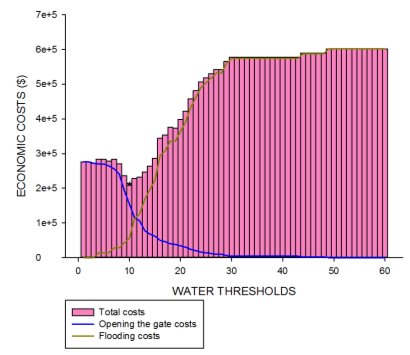
Figure 9: Opening gate curve (blue), flooding cost curve (brown) and bar graph of total cost for different water thresholds considered (from 1 to 60).
Discussion
To make the previous forecasts, a 1-D hydrodynamic flood routing model with simulated flood peaks was used. This data is easy to acquire and therefore this procedure can be simply implemented. The assumptions considered for the 1-D hydrodynamic model are: 1) the flow is one-dimensional (velocity is uniform across the cross-section); 2) there are no vertical accelerations; 3) hydrostatic pressure distribution (water level across any cross-section is horizontal); 4) the bottom slope of the channel is small; 5) boundary friction and turbulence are represented by a resistance force using uniform flow expressions (Hewett, 2018). Also, for its application, a calibration of the model parameters with observed data has to be done. To be operational for real-time flood forecasting, a verification and validation (based on how well the model performs in triggering alarm thresholds correctly and in predicting the timing of alarms correctly) of the model is also needed. It has to be kept in mind that the results obtained are just indicative, due to this, modern approaches use varying parameters and offer a range of solutions, not just a unique one. Nevertheless, modelling gives an insight of the problem that can be more important than the final result (Hewett, 2018).
Thresholds are a critical element in flood forecasting, as a warning is issued if the discharge is higher than a predefined threshold (Weeink, 2010). With the aim of defining an optimal threshold, index values as POD, FAR, CSI, and costs were considered.
When we consider the index values, the threshold that optimizes our forecasting is 13 m3s-1. The FAR is equal to 0.205, close to 0, which means that the false alarms emitted are low. The POD is 0.721, which means that the hits ratio is high (close to 1). Finally, the best CSI is equal to 0.608, this was the higher value obtained for all the thresholds. It is a more balanced score and indicates that a high amount of forecasted “yes” events corresponded to the observed “yes” events. By using this threshold value we optimize our forecasting as we win quality and consistency; defined as the degree to which the forecast corresponds to what actually happened and the correspondence between forecaster’s best judgment about the situation and their forecast, respectively. Therefore, a major amount of mistakes is avoided and we don’t create false expectations on people. They’ll trust the forecast more and we’ll be willing to take the correspondent actions when needed.
On the other hand, if we consider the costs that come with opening or not the gate, the best model threshold would be 10 m3s-1. By using this threshold we gain value, defined as the degree to which the forecast helps the decision maker to realize some incremental economic and/or other benefits. Costs are minimized as less severe damages occur.
To finish, a probabilistic forecast should be incorporated. This way, the decision process can be backed up with probability distributions. Although this could lead to a more risk-averse attitude, fewer errors are made when it is considered.
Conclusions
To sum up, even if the model was optimized to the maximum and the forecasts were precise, to obtain real results society has to be educated about the issue. To be effective, the actors involved in the hazard area should be organized and well prepared. The information should be easily available to the authorities and good communication channels should exist; the entire warning chain should be in perfect conditions. The goal is that, by good communication and educational campaigns, to minimize under and overreaction to risks and to influence peoples’ willingness to behave adequately and invest in prevention measures.
References
Hewett, C., 2018. Hydraulic Flood Routing ModelsModelling.
CEH, C. for E. and H., 2018. National River Flow Archive [WWW Document]. URL http://nrfa.ceh.ac.uk/data/station/info/52010 (accessed 3.19.18).
EAAA, E.A.A. yr A., 2012. Flood Estimation Guidelines.
Ewen, J., Parkin, G., O’Connell, P.E., 2000. SHETRAN: distributed river basin flow and transport modeling system. Journal of hydrologic engineering 5, 250–258.
Kilsby, C., 2018. Rainfall Forecasting.
Kjeldsen, T.R., 2007. The revitalised FSR/FEH rainfall-runoff method. NERC/Centre for Ecology & Hydrology.
Mellor, D., Sheffield, J., O’Connell, P.E., Metcalfe, A.V., 2000. A stochastic space-time rainfall forecasting system for real time flow forecasting II: Application of SHETRAN and ARNO rainfall runoff models to the Brue catchment. Hydrology and Earth System Sciences 617–626.
O’Connell, E., 2018a. PredictiveUncertainty2018.
O’Connell, E., 2018b. Rainfall-runoff Modelling for Real-time Flood Forecasting.
O’Connell, E., O’Donnell, G., 2018. VIRTUAL FLOOD: A simulated flood event and warning exercise.
Shaw, E., Beven, K.J., Lamb, R., Chappell, N.A., 2014. Hydrology in practice. CRC Press.
Todini, E., 2009. Predictive uncertainty assessment in real time flood forecasting, in: Uncertainties in Environmental Modelling and Consequences for Policy Making. Springer, pp. 205–228.
Todini, E., 2008. A model conditional processor to assess predictive uncertainty in flood forecasting. International Journal of River Basin Management 6, 123–137. https://doi.org/10.1080/15715124.2008.9635342
Tucci, C.E., 2003. Flood flow forecasting. Bulletin of the World Meteorological Organization 52, 46–52.
Wallingford HydroSolutions Ltd, 2009. WINFAP FEH3-UserGuide.
Weeink, W.H., 2010. Evaluation of streamflow and ensemble tresholds (Master’s Thesis). University of Twente.
Cite This Work
To export a reference to this article please select a referencing stye below:
Related Services
View allRelated Content
All TagsContent relating to: "Environmental Science"
Environmental science is an interdisciplinary field focused on the study of the physical, chemical, and biological conditions of the environment and environmental effects on organisms, and solutions to environmental issues.
Related Articles
DMCA / Removal Request
If you are the original writer of this dissertation and no longer wish to have your work published on the UKDiss.com website then please:


