Effects of Hydrostatic Pressure on the Burst and Collapse Behaviour of Marine Pipelines

ABSTRACT

When a pipeline is submerged through different levels of water depth for use in offshore applications, it experiences the effects of high pressure variations resulting in net external or internal loads. If such loads exceed a critical value, the marine pipeline may undergo permanent deformation or even complete failure, subsequently causing high safety risks and major loss in revenue to all involved. The mechanical behaviour under high net loads acting externally and internally must therefore be studied to understand which adjustments must be made in order to prevent these events from occurring. This work will carry out a numerical and computational study to a) produce theoretical solutions to find effective parameter changes which can be made to prevent undesirable behaviour, b) find the effects of pressure on the mechanical behaviour of pipelines with initial ovalities, validated by c) a simulation using various conditions of the marine pipeline in order to find the maximum values of stress present in the model.

1. Introduction

1.1 Background and Literature Review

There is a rapidly ever-increasing demand for more energy around the globe, and due to the continual depletion of easily accessible oil reservoirs, engineers are tempted to expand the reach of ocean facilities into remote locations in far deeper waters than before (Salama et al., 2000). This increases concern to the safety of all personnel involved in operating such equipment and runs the risk of extreme environmental pollution should any failures occur.  Of course, in far deeper waters brings far harsher environments and increasing loads, putting extra strain on subsea equipment. However, there are not only high safety risks to personnel involved, but also detrimental impacts to the company’s revenue should the occurrence of a failure happen. It is therefore a necessity to consider the costs involved in maintaining and repairing damaged equipment and so, focus must be put on preventing these events happening in the first place.

Failures may occur to a pipeline for a number of reasons; primarily high mechanical loading as a result of extreme net pressures acting internally or externally, and environmental conditions such as corrosion, temperature, and water diffusion (for example, Assarar et al., 2011, Pauchard et al., 2002) – the latter being a fairly revised subject due to a relatively consistent spread of conditions throughout currently ongoing offshore operations. However, failure due to extreme loads at deep sea has been considered notably less until recent years where engineers have been making huge leaps in the design of offshore facilities in far deeper waters than before. Therefore most of the material produced in this field has been written many decades ago, before scientists even considered that it were possible to reach water depths in excess of 2500m.

Recent studies have shown that corrosion is the cause of 36% of subsea pipeline failure as opposed to only 13% being to material failure under high loads (Yang et al. 2017). It may be true in saying that corrosion plays a pivotal role in decreasing surface thickness however, high loads must also be simultaneously applied for the pipe surface to break and therefore, equally important to consider.

There have been many cases of previous research into the understanding of mechanical behaviour of pipelines due to hydrostatic pressure. However, many of these reports haven been specific to a defined material. More specifically, ‘The Mechanical Behaviour of Materials Under Pressure’ (Vodar and Kieffer, 1971) was amongst the earliest to perform tests on the effects on metallic materials, and similar tests being held more recently (Wu et al., 2009, Zhang et al., 2017). It is worth noting that the large time gap between studies shows that research into this field is still needed and of interest in the present day. A fair amount of research has also looked into the effects of mechanical loading on composite cylindrical structures (for example, Hine et al., 2005, Davies, 2016), but considerably less on titanium and aluminium – likely due to high economical expenses. Despite such a wide range of knowledge in this field, there have been very few direct comparisons between materials with respect to ocean applications, and this report intends to expose these knowledge gaps.

Studies similar to the one carried out in this work exist publicly but with some uncertainties in the accuracy of the work. One previous study in particular describes a collapse test with ovality in the pipe circumference by modelling a half circumference to represent symmetry on one axis (Kaviti et al., 2013). The geometry however, follows a biconvex shape as opposed to an oval, meaning if the shape were to be reflected it would appear to have two seems on either side, without stating this was intentional. The effect of this would mean a likely increase in maximum stress by a considerable amount and therefore, an improved geometry definition may be needed.

Selecting the correct material to use is one of the most fundamental disciplines in engineering. It determines the reliability of the design in terms of safety and economic viability. So of course, it is vital to have a vast range in knowledge of different materials and an open mind set into exploring new ones. The main considerations are focused on the properties of each material and its ability to withstand various loads. The specification and use of materials which combine high mechanical strength with corrosion resistance and resistance to wear is a fundamental requirement.

An example of insufficient material usage comes from the North Sea, where the Norwegian Petroleum Directorate (NPD) has expressed their concern about recent experiences with respect to material selection and safety. Gas leakages, albeit very small, have been reported to stand at over 220 during the period of 1996 to 2002 (Lange and Berge, 2004).  Many of these leakages come from failures in subsea pipelines through pipe wall fractures, which could possibly have been resolved had a more appropriate material been chosen. Luckily, none of these caused significant damage; however, it still holds the potential for danger to the lives of operating personnel and marine life. This is why material selection is vital. Furthermore, it is estimated that roughly half a billion pounds (including loss of income) was lost due to these failures. Such significant loss of revenue puts high demand on the correct selection of materials.

As it stands, API 5L X65 steel linepipe is the most commonly used steel grade in the offshore industry however, extensive research is looking into the possibilities for using more advanced materials to meet industries demanding needs. In North America and China the X80 steel linepipe is on the rise with approximately 10,000km of offshore pipelines in each continent being used as of 2012, while North America are currently in the process of trialing the X100 linepipe (Sung, 2012). From this evidence it is clear that giving accurate relevant performance comparisons between materials should be given full consideration.

1.2 Research Idea, Aim and Objectives

As ocean structures and the marine pipelines which link these to onshore facilities are being pushed to operate in far deeper waters, we must fully understand the effects of increasing hydrostatic pressures to effectively design pipelines in high-pressure situations. Following this, the report aims to focus on the effects of mechanical loading on a variety of selected materials by understanding the changes in mechanical behaviour of marine pipelines caused by extreme hydrostatic and internal pressures.

The initial aim is to provide accurate relationships between the most influential parameters which affect the mechanical behaviour of pipelines in order to prevent failure. These results will then be validated by giving a finite element model solution to prove that the values will prevent the pipeline from ever exceeding the maximum allowable operating stress. Finally, the importance of the most influential parameters will be emphasised to show why careful control must be kept in retaining allowable values, such as diameter to thickness ratio and initial imperfections in pipe ovality.

Engineers wishing to design ocean structures and in need of relevant information of material performance  and adjustable parameters for effective design may use this piece of work as a general reference for values such as maximum operating pressure and required diameter to thickness ratio which should be used. Thereby, this work should provide a valuable stepping stone to engineers who wish to better their general understanding in the field and provide as a valuable teaching resource for the way a marine pipeline behaves subject to high mechanical loading whilst varying the most influential factors. This will also aid engineers to understand why consideration must be given in the design process to durability, safety and economic viability. By reducing these knowledge gaps we therefore hope to reduce the risk of incidents in marine pipelines. Furthermore, the model was designed with a single material cylindrical shell therefore, the basic principal of this project may be used for learning purposes when considering a variety of applications such as marine risers and casing and tubing of subsea wells.

1.3 Overview of Contents

Collaboration of simplified databases will be given with information on materials which are most commonly used in ocean appliances, such as pipelines/flowlines and marine risers. This will comprise of a selection of 5 different steel grades most commonly found in offshore appliances, namely, API 5L X Grades. Conclusions will be made in the latter stages of the report of the found advantages over one another in terms of resistance to high net pressures, safety and economic viability.

This will be followed by calculations to estimate the magnitude of forces which pipelines undergo in an offshore environment; primarily being hydrostatic pressure. This will allow us to understand the pressure variations at each level of water depth and therefore, the variation of forces imposed on pipelines.

The next section will include wall thickness calculations subject to imposing pressures only at water level. This will be enough to calculate the maximum thickness for burst, however, to estimate thicknesses to prevent collapse, the pipe will be subject to a variation of high hydrostatic pressures as water depth increases. By initially keeping the thickness constant as it varies through water depth, we can observe when the collapse pressure safety check is not satisfied and the adjustments we need to make to the wall thickness. Furthermore, these results will be validated using the ANSYS Mechanical 16.0 software.

The adjustments needed to be made to prevent collapsing of the pipe with initial imperfections will then be examined, which will be done with imposing hydrostatic pressure through a variation of ovality percentages. This will allow conclusions to be made on the acceptability of allowable ovality in the pipe cross-section and the acceptable water depth at which a pipe with said ovality may operate. These results will also be validated by using the ANSYS Mechanical 16.0 Software.

2. Theoretical Solutions to Prevent Failure

2.1 Materials for Pipeline Design

The focus of material selection will be associated for use with offshore line pipes – a high strength high yield carbon steel pipe used for transporting crude oil, natural gas and water.

The main factors which influence the selection of materials for this type of application are: the physical and mechanical properties of the material; its resistance to corrosion against the environment and a wide range of operating conditions; its resistance to marine biofouling; and its ability to perform fabrication operations – all of which contribute in some form to the safety aspects of using such materials and to economic considerations. The main focus of the content in this report will focus on the physical and mechanical properties of the material with respect to how they change under high loading, the rest of these factors are considered to be outside the scope of work in this project.

Line pipes make up the vast majority of the market for offshore pipelines – most commonly fixed to the seabed. There are many pieline standard codes used around the world, with the most common ones being, American Natl. Standards Inst. (ANSI), American Soc. of Mechanical Enginers (ASME) and Det Norske Veritas, Norway, and Germanischer Lloyd, Germany (DNV GL) however, the majority of codes used in this report will be under regulations specified by the American Petroleum Institute (API) which defines the API Specification 5L standard used worldwide. Pipes can be either welded or seamless, however, the great advantage of the seamless pipe is its ability to withstand pressure as opposed to a welded pipe which have considerable weaknesses along the welded seam. For this prime reason, we will consider seamless pipes to give a superior performance and will be used in the following methods.

The thermophysical properties of the materials are neglected with the assumption being made that the ductile to brittle transition temperature will never be reached (roughly -80ºC) and that steels can withstand temperatures in excess of 300ºC without being affected, therefore, in this instance temperature is outwith the scope of this work. Table 2.1 presents mechanical properties of a selection of the most common materials used in line pipes as specified by API.

Steel Grade (API 5L)	X52	X56	X60	X65	X70
Min. Yield Strength (ksi/MPa)	52/359	56/386	60/414	65/448	70/483
Min. Tensile Strength (ksi/MPa)	66/455	71/489	75/517	77/531	82/565

Table 2.1 – Steel grade and corresponding yield and tensile strengths.

The following methods will use values associated with steel grade API 5L X65, however, values can be easily interchangeable and are given in Table 2.1 for a fuller range of materials which will also be analysed theoretically.

2.2 Internal and External Pressure

As the subsea pipeline is submerged in water to deep sea conditions, it naturally experiences continual variations in external pressure, due to the pressure within the liquid, the acceleration due to gravity and the depth within the liquid, as stated by Pascal’s Principle. If the internal pressure is kept at constant throughout, either being atmospheric pressure (empty) or operating pressure, then net pressures will vary linearly with water depth. The combination of high internal pressure and low external pressure will result in an externally acting force – which if large enough will cause the pipe to burst. Similarly, the combination of low internal pressure and high external pressure will result in an internally acting force – which if large enough will cause the pipe to collapse. This is the basis of the mechanical behaviour which we shall be looking at. It is worth noting that the internal pressures of a pipe can be controlled and set manually to an extent; whereas the prime source of external pressure is hydrostatic which occurs naturally as stated previously. For safety measures, we shall consider the unusual case where internal pressure cannot be carefully controlled and will be kept unpressurised in the following collapse tests to represent the most extreme case occurring.

2.3 Hydrostatic Pressure

Hydrostatic pressures experienced at deep sea can have detrimental effects on the mechanical behaviour of pipes. The classical form of Pascal’s Principle may be used to give sufficient estimations of imposing pressures formed at extreme water depths, carrying forward the assumption that the fluid is at rest and is incompressible. Such assumptions may give inaccuracies in exact water pressures as these are rarely the case however, greater accuracy is not needed to obtain relevant conclusions in this study. Pascal’s Principle states that the pressure within a liquid depends on the density of the liquid, the acceleration due to gravity, and the depth within the liquid.

PExternal=PAtmoshpere+PFluid

(1)

PFluid=ρgh

(2)

Where, atmospheric pressure is

101kPa, the density of seawater is

1.025 g/cm3and the standard local gravity is

9.80665 m/s2. Water depth,

h, is varied from the water level to

3000mto accommodate applications ranging from shallow to the deepest of waters. The external pressure will be represented by

PO. The following external pressures were achieved in order to represent the linearly external loads experienced by subsea pipelines, as seen in Table 2.2.

Water Depth (m)	0	500	1000	1500	2000	2500	3000
External  Pressure (kPa)	101	5127	10153	15179	20205	25231	30257

Table 2.2 – External pressure variation with water depth (Atmospheric and Hydrostatic).

2.4 Pipe Wall Thickness

The main parameters which strongly influence the behaviour of thick-walled pipes are material properties, net pressure, the outer diameter to thickness ratio,

DO/t, and imperfections, such as the initial ovality.  Each of the mentioned parameters will be considered as variables to combat the effect of excessive net pressures acting on a cylindrical shell as it is submerged through a range of water depths.

Initially, the outer diameter to thickness ratio,

DO/t, will be calculated suited for a pipe which lies above sea level and kept constant as the pipe experiences the effects of submergence in sea water. Thereby, allowing us to understand the adjustments needed to be made to repel deformation of the shell as the external pressure ranges through deep sea imposing high loads. Wall thickness calculations can be made in accordance with the ANSI/ASME Standard B31.3 code – an extension of Barlow’s Formula to allow for high safety margins, such as corrosion allowance, te, given as

0.079in(2mm) as a general guideline for steel pipes carrying crude oil, and a value of

0.05in(1.27mm) is used for the thread or groove depth,

th, in accordance with the pipe nominal size. We will also use an outside diameter,

DO, of

10in(254mm) for the test pipe and therefore, the manufacturer’s allowable tolerance,

ttol, is

12.5%for API 5l steel pipes up to

20in(508mm) diameter, giving us the following expression for minimum design wall thickness

t=te+th+PIDO2SE+PIY100100-Ttol

(3)

Where, longitudinal weld-joint factor,

E, is set at a value of

1.0for a seamless pipe and a derating factor,

Y, is set at 0.4 for ferrous materials operating below

900oF. The maximum allowable internal pressure in the pipe,

PI, is set at a constant initial value of 2500psi (17,237kPa).

And

Sis the allowable stress for the pipe, taken as the Specified Minimum Yield Strength (SMYS) of the material which is the limit of elastic deformation.

2.5 Burst and Collapse Pressure

Theoretical solutions are proposed for the elastic burst and collapse pressures to prevent yielding of a cylindrical shell exposed to uniform internal and external pressures. It is noted that the main cause for failures to occur be that the internal pressure exceeds external pressure, or vice versa, by a substantial amount given by the product of some factor, f0, giving way for a safety allowance, and the critical pressure to cause collapsing or bursting of the pipe.

It should be noted that in this report, the burst and collapse term is used to differentiate between the yielding pressure in that relative motion. For example, the pipe will not completely burst or collapse until the ultimate tensile stress has been reached, however, values of maximum stress used in the following methods will relate directly to the value of yielding stress. Beyond this point the model will begin to plastically deform and so we will deem it to have failed and therefore the maximum allowable stress is the point of yielding. Should we achieve resultant values greater than the point of yield, previous studies (Toscano, 2009) state that disregarding the steel work-hardening of a material in the plastic transition zone has a neglible effect on the burst and collapse pressures and therefore, the same equation used to calculate stress values in the perfectly elastic zone will be assumed to also give accurate results when determining failure.

And so, in accordance with API-1111 the critical failure pressure of the pipe must exceed the net pressure everywhere along the pipe and is expressed as follows

PI-PO≤f0 Pbr

(4)

PO-PI≤f0 Pc

(5)

Where,

PIis the internal pressure of the pipe which will range from atmospheric pressure (depressurised) to a maximum operating pressure of

2500psi. For safety measures, collapse pressure checks will be made with respect to the condition where the pipe is empty (unpressurised), and burst pressure checks to the maximum operating condition.

Pbrand

Pcare burst pressure and collapse pressure of the pipe, respectively. All values of pressure used must therefore be given as positive to comply with the previous expressions.

We can calculate the ultimate burst pressure,

Pbr, by using the following formula in accordance with API-1111 as follows

Pbr=0.45 S+Uln⁡DODI

(6)

Where,

Sis the specified minimum yield strength and

Uis the specified minimum ultimate tensile strength which is given in Table 2.1, and

DI=DO-2t. This relationship is needed as pipe burst does not occur precisely at the yield or ultimate tensile strength.

Figure 2.1 shows an offshore pipeline pipe wall fracture due to bursting motion. This was achieved with extreme internal pressures causing the pipe material to reach the ultimate tensile stress, causing complete failure, as opposed to yield stress which would only result in permanent deformation.

Figure 2.1: Pipe Burst due to Large Internal Pressure.

Source: Gajdoš and Šperl (2012) Figure 16 ‘Evaluating the Integrity of Pressure Pipelines by Fracture Mechanics’ Academy of Sciences of the Czech Republic, Czech Republic.

It must be noted, bursting of a pipeline is entirely a problem of an internal pressure which creates a stress in exceedance of the maximum stresses allowed. Once calculating the wall thickness to diameter ratio which will achieve 72% SMYS with respect to the applied internal pressure, it can be assumed that the pipeline will never veer close to bursting. Instead, this work shall aim to optomise the maximum allowed internal pressure by achieving equilibrium with the opposing hydrostatic pressure as the water depth is increased.

Relating back to equation (4), we can substitute in the burst pressure value while varying the external pressure accordingly with Table 2.2 and keeping the internal pressure constant as the maximum operating pressure throughout. We are reminded that equation (4) states the following:

PI-PO≤f0 Pbr

Where,

f0 represents a series of factors for example, the temperature derating factor,

ft as specified by API-1111 as 1.0, the longitudinal weld joint factor,

fe also being 1.0 for a seamless pipe, and the internal pressure (burst) design factor,

fd being 0.9 for pipelines. According to most safety standards around the world, this safety factor of design stress should stand at around 72% of the specified minimum yield strength; however, since the burst formulation is given with respect to the ultimate yield strength,

f0 will stand at a value of around 65%.

Since now knowing all factors in equation (4), we can observe if this is satisfied for all water depths and variations in external loads by checking that the hydrostatic test pressure (internal minus external pressure) never exceeds the product of the safety factor and the burst pressure. The values in Table 2.3 represent the required wall thickness at the maximum value of

PI-PO,being 2,500psi (17,237kPa), and if the following ANSYS validation proves equation (4) to be satisfied, then we shall assume the equation will also be satisfied for all values of water depth.

Steel Grade (API 5L X)	52	56	60	65	70
Minimum Wall Thickness (mm)	10.160	9.652	9.114	8.890	8.382
Minimum   DO/t	25.11	26.36	27.55	28.97	30.31

Table 2.3 – Minimum wall thickness at water level to prevent burst.

We can calculate the collapse pressure,

Pc, by using the following formula in accordance with API-1111

Pc=Py PePy2 + Pe2

(7)

Where

Py is the yield pressure at collapse and can be calculated as follows

Py=2 S tDO

(8)

And

Pe is the elastic collapse pressure of the pipe and is given as

Pe=2 E tDO31-v2

(9)

Where the modulus of elasticity

E=3∙107psi ( 207GPa)a and Poisson’s ratio for steel,

v=0.3. Since all values are know we can substitute these into equation (7) to obtain the collapse pressure of the pipeline.

Figure 2.2 represents an offshore pipeline which has collapsed due to extreme hydrostatic pressures causing the pipeline material to exceed the yield stress.

Figure 2.2: Pipe Collapse due to Large External Pressure.

Source: Paschoa C (2013) Untitled ‘JIP Collapse Assessment of Offshore Pipelines with D/t <15’ Marine Technology News.

Similarly to the previous Burst Safety Check, we can use safety measures to check for the possibility of collapsing. If we refer back to equation (5) again where we have the following for collapse

PO-PI≤f0 Pc

Where,

f0 represents the collapse factor and is given as a summative value of 0.65 – with respect to the UTS, meaning that the stress obtained by the difference in external pressure should never exceed 72% of the SMYS. Again, we will check the equation is satisfied for all water depths and variations of external pressures.

By using the safety check, we can find out when the collapse pressures fail to meet this criteria and how they can be modified to satisfy the equation. We can gain an iterative solution firstly, by increasing the outer diameter to thickness ratio,

DO/t, and finding out which values satisfy the equation for each value of water depth and similarly, if the equation is already satisfied for values of water depth we can decrease the diameter to thickness ratio as the excess material will be unnecessary and will further reduce costs. On doing this, we will know the required minimum wall thickness for each water depth, as seen in Table 2.4.

Water Depth	1000	1500	2000	2500	3000
Minimum Wall Thickness (mm)	3.96	5.93	7.91	9.88	11.87
Minimum   Do/t	64.2	42.8	32.1	25.7	21.4

Table 2.4 – Minimum required wall thickness for selected water depths for API 5L X65.

The values presented in Table 2.4 correspond to

Do/tratios for steel grade API 5L X65. It can be seen that the jump between ratios slowly decrease as water depth is increased. The same method was used to calculate values for all materials as discussed in section 2.1. These values will be validated by ANSYS Mechanical in the next section.

2.6 Collapse Pressure with Initial Ovality

As well as the outer diameter to thickness ratio, initial imperfections also strongly influence the collapse behaviour of pipes. For this section we shall ignore the effects of ovality on burst pressure as it has very little effect due to the pipe shell likely returning to its original shape before bursting. Many literatures agree on the importance of initial ovality,

∆0, on the collapse behaviour of pipe material and the definition described in previous studies (Corona et al., 1998) is expressed by the following equation

∆0=DMAX-DMINDMAX+DMIN                            (10)

Where

DMAX is the maximum diameter at cross section and

DMIN is the minimum diameter. The degree of ovality is determined by the difference between the maximum and minimum diameters divided by the nominal diameter of the pipe and so, the percent ovality is expressed as follows

∆%=DMAX-DMIND∙100

(11)

Where the nominal diameter of the pipe is given as follows

D=DMAX+DMIN2

(12)

For the purpose of the experiment the percentage of initial ovality will be varied from 2 to 10 in steps of 2% to determine if the collapse pressure will be reached.

There were early studies on the collapse behaviour of pipes under external loading (Timoshenko and Gere, 1961) which took into consideration the initial imperfections such as ovality. They produced a design formulation for calculating collapse pressure which takes the following form

PC=12Py+μPe-Py+μPe2-4PyPe12

(13)

Where the yield pressure,

Py, follows the same form as equation (8) and the elastic collapse pressure,

Pe, is also given by equation (9). In the case were the circumference is perfectly round, the elastic-collapse pressure plays an almost neglible role and the collapse pressure becomes close to the value of yield pressure. The ovality coefficient is given as follows

μ=1+3∆0DOt

(14)

The final results will be used to show the differences in collapse pressures with various initial ovalitys.

3. Results of Theoretical Solutions

The previous numerical equations were used to find solutions to prevent the burst or collapse of marine pipelines by considering the most influential parameters, such as diameter to thickness ratio and initial imperfections. The API-1111 code for burst and collapse and the expression, for collapse pressure with an ovality factor, defined earlier (Timoshenko and Gere., 1961) were used to create the relationships as seen in section 3.1 in order to describe the minimum allowed values which must be used in pipeline design to prevent failure. The figures show each of the steel grades discussed previously, as well as additional material references which are currently in a ‘trial’ stage across the industry. For instance, the number of titanium and titanium alloy applications are increasing at an exponential rate across the oil and gas industry, particularly in the Norweigan sector of the North Sea, due to its widely known advantages over steel in terms of corrosional resistance against sea water and petroleum products. Therefore, it will be very benifical to establish any advantages of these ‘trial’ materials over more widespread materials in the industry.

3.1 Parameter Relationships to Prevent Failure

The following graph was presented to show that the internal pressure can be increased with each depth of water in order to resume equilibrium on the resultant hydrostatic pressure force.

Figure 3.1 – Allowable Internal Pressure Increase per Water Depth

The values of internal pressure shown in Figure 3.1 were calculated as the maximum allowable internal pressure before the design limit of 72% SMYS is exceeded. Each steel grade was given the same values of diameter to thickness ratio which remained constant throughout the submergence of the pipe to give a relative comparison of strength performance.

The next relationship that was created shows the amount by which you must decrease the diameter to thickness ratio for each level of water depth.

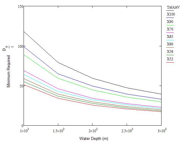
Figure 3.2 – Required Diameter to Thickness Ratio for each Water Depth

The values of diameter to thickness ratio shown in Figure 3.2 are the minimum required values in order to prevent the pipe from collapsing due to hydrostatic pressure. As briefly discussed previously, the internal volume was depressurised and held constant at a value equal to atmospheric pressure throughout.

Lastly, the following graph shows the effects which the ovality percentage of the circumference of a pipeline has on it’s collapse pressure.

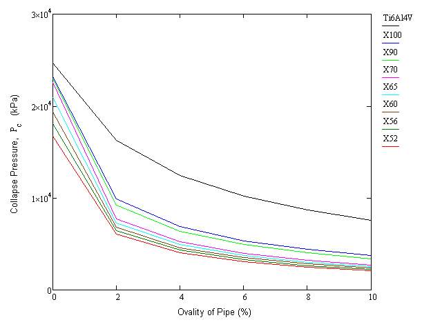
Figure 3.3 – Collapse Pressure Against Percentage of Ovality

The collapse pressure shown in Figure 3.3 shows the pressure at which the pipeline yields. Beyond this, stress values will enter the plastic-elastic zone and permanent deformation will occur, thus the model will be deemed to have failed beyond this point.

4. Finite Element Model

The ANSYS Mechanical 16.0 software programme was used to develop a two dimensional cross section of a cylindrical shell, subject to internal and external pressures varying with water depth. It is noted that, although a three dimensional model would describe a more complete picture of the mechanical behaviour of the pipeline, two dimensional models are extremely useful in predicting the different weighting of factors which affect the burst and collapse behaviour of pipelines. For example, if we refer back to Figure 2.1 in Chapter 2, you can observe that the point of burst would be somewhere roughly in the middle of the propagated crack; however, this work aims to prevent failure from occurring at any point along the length of the pipe and therefore three dimensions will not be needed. For this reason, we will also not consider stiffening equipment, such as buckle arrestors, which may lie on the longitudinal axis. A total of 15 models, 5 of each of the previously mentioned relationships, will be modelled and simulated under the conditions which were used to produce them. Input data for each model was taken directly from the theoretical results used to present relationships 3.1, 3.2 and 3.3.

The procedure is based on the finite element method and is used to estimate if the load bearing capacity of high pressures acting internally or externally on the pipe wall will be reached or exceeded when using the calculated parameter values for each model. If the critical pressures are not reached – but come considerably close, then the theoretical solutions to prevent failure will be validated. Following this, the pipe will be modified to determine the effect of pressure on the mechanical behaviour of pipelines with initial imperfections to validate the theoretical solutions of preventing collapse in a pipeline with ovality in it’s circumference. As the maximum allowable pressures were calculated with a factor of 0.72, we shall expect to find that the maximum stress in each case reaches 72% SMYS.

Some minor difficulties which come with using ANSYS Mechanical is that the software cannot easily visualise pipe burst or collapse – it will treat the material as a perfectly elastic model no matter what the achieved stress is; instead it will provide data to obtain the maximum stress occurrence in each model which we can compare with the maximum allowable yield and ultimate stress for each case. This is suitable for the purpose of this project as the von Mises stress can be used to calculate maximum stress values up until the point of yielding, and the main aim in this study is to prevent stress values exceeding this point.

Further errors may arise in the modelling of a pipe with ovality. For example, some previous studies use quarter or half pipe cross section models where ends do not meet the symmetry plane with right angles, meaning should the shape be reflected on the symmetry planes, the end result would be a curved-quadlerateral shape. The full effect of this is unknown, however, stress values will most definetely be different to those of a perfect elliptical shape as the initial geometry. Thereby, the models used in this report aim to have the element edge which is joined to the symmetry plane as close to 90º as possible.

4.1 Model Geometry

As mentioned previously, the simulations on ANYS Mechanical will be used to validate the theoretical results obtained in the previous section as represented by Figures 3.1, 3.2 and 3.3. These will consist of determining if the maximum allowable stress for burst, collapse, and collapse with initial ovality is exceeded or if the results are consistent with those obtained theoretically.

For the case of examining if the critical stress to cause pipe burst is reached, the pipe cross-sectional model will be simulated subject to the pressures experienced at the water level with an internal operating pressure of 17236kPa and atmospheric pressure being the external force. A further 4 simulations will be made by increasing the external pressure accordingly with the hydrostatic pressure present at each water depth and simultaneously increasing the internal operating pressure of the pipe to a value which returns the pressure forces to equilibrium. The aim will be to show that the maximum internal operating pressure at the waterline may be inceased further due to the increased external resistance force for a constant diameter to thickness ratio. Table 4.1 shows the input data for the burst simulation.

Pipe Parameters	Case 1	Case 2	Case 3	Case 4	Case 5
Pipe Material	API 5L X65
Water Depth (m)	0	500	1000	1500	2000
Outer Diameter (mm)	254	254	254	254	254
Wall Thickness (mm)	6.78	6.78	6.78	6.78	6.78
Inner Diameter (mm)	240.44	240.44	240.44	240.44	240.44
External Pressure (kPa)	101	5127	10153	15179	20205
Internal Pressure (kPa)	17338	22364	27390	32416	37441

Table 4.1 – Input Data for Burst Test.

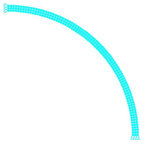
Figure 4.1 – Finite Element Mesh with Boundary Conditions (Case 5)

Figure 4.1 shows a sample of the finite element mesh of the model from Case 5. It is defined by 324 nodes and 240 elements, with the nodes on the y-axis symmetry plane given a zero displacement in the x direction (left hand edge) and the nodes on the x-axis symmetry plane given a zero displacement in the y direction (bottom edge).

For the case of examining if the critical stress to cause collapsing is reached, the finite element model of the cross-sectional area of the pipe will be simulated with a sample of 5 models, those being the API 5L X65 material and its corresponding required outer diameter to thickness ratios for 1000m to 3000m depth. If all are validated and correct i.e. maximum allowable yield and ultimate stresses are not exceeded for each case, then we can assume all other values for each material will also be correct. It is initially modelled by defining the outer and inner diameters of the cross sectional area of the pipe, the inner being the subtraction of the outer diameter and the previously calculated wall thickness. Each model will be given a 10in (254mm) diameter with an inner diameter relevant to the calculated required wall thickness for the associated material subject to varying hydrostatic pressures. The aim will be to show that the relationship seen in Figure 3.2 representing diameter to thickness ratio varying with water depth to prevent the yield stress being reached is correct. Table 4.2 shows the input data for the collapse simulation.

Pipe Parameters	Case 6	Case 7	Case 8	Case 9	Case 10
Pipe Material	API 5L X65
Water Depth (m)	1000	1500	2000	2500	3000
Outer Diameter (mm)	254	254	254	254	254
Wall Thickness (mm)	3.96	5.93	7.93	9.88	11.87
Inner Diameter (mm)	246.09	242.13	238.17	234.17	230.26
External Pressure (kPa)	10153	15179	20205	25231	30257
Internal Pressure (kPa)	101	101	101	101	101

Table 4.2 – Input Data for Collapse Test.

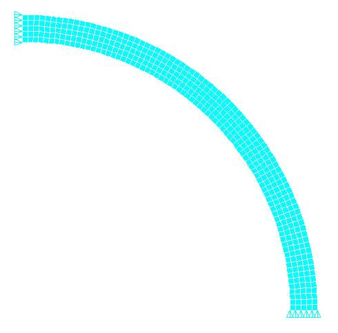
Figure 4.2 – Finite Element Mesh with Boundary Conditions (Case 10)

Figure 4.2 shows a sample of the finite element mesh of the model from Case 10. It is defined by 486 nodes and 400 elements, with the nodes on the y-axis symmetry plane also given a zero displacement in the x direction (left hand edge) and the nodes on the x-axis symmetry plane given a zero displacement in the y direction (bottom edge).

For the case of examining collapse pressure with an initial ovality in the pipe cross-section, a further 5 models will be created with initial ovality varying from 2 percent to 10 percent and similarly to the previous tests, steel grade API 5L X65 will also be the only material used to reduce computational time. This model will be given a fixed nominal diameter to thickness ratio throughout corresponding to that needed at 3000m, as we will achieve better results with an increased external pressure. The assumption is also made that thinning and thickening in the pipe wall thickness is not present to begin with and therefore, pipe wall thickness remains constant. The aim is to find out the ovality acceptability i.e. if the allowable stress in the model will be reached in each case. Table 4.3 shows the input data for the collapse with initial ovality simulation.

Pipe Parameters	Case 11	Case 12	Case 13	Case 14	Case 15
Pipe Material	API 5L X65
Water Depth (m)	521	358	268	217	182
Inner Dmax (mm)	240.44	250.60	260.76	270.92	281.08
Inner Dmin (mm)	220.12	209.96	199.80	189.64	179.48
Wall Thickness (mm)	11.87	11.87	11.87	11.87	11.87
Outer Dmax (mm)	264.16	274.32	284.48	294.64	304.80
Outer Dmin (mm)	243.84	233.68	223.52	213.56	203.20
External Pressure (kPa)	5347	3706	2796	2283	1936
Internal Pressure (kPa)	101	101	101	101	101
Percent of Ovality	2	4	6	8	10

Table 4.3 – Input Data for Collapse Test with Initial Ovality

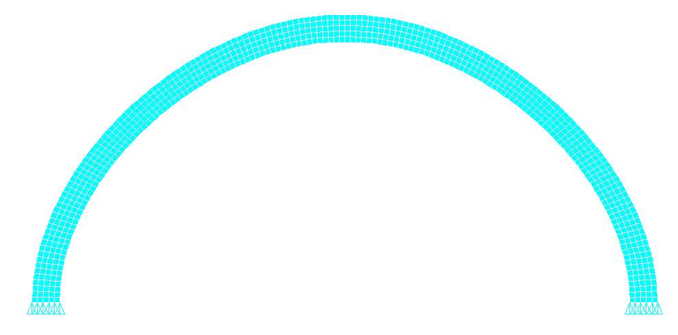
Figure 4.3 – Finite Element Mesh with Boundary Conditions (Case 11)

Figure 4.3 shows a sample of the finite element mesh of the model from Case 11. It is defined by 960 nodes and 790 elements, with the nodes on the x-axis symmetry place given a zero displacement in the y direction (bottom edge). Cases 11-15 were modelled by using a half circumference cross section, as opposed to the quarter circumference model used in the previous tests, as 4 key points were needed around the centre point to model the 180º arc and cutting the geometry in half following this would be unnecessary. The purpose of doing so was to assure that the distance from the centre point to any element would never be outwith the range of the minimum input radius and the maximum input radius.

4.2 Simulation Setup

For each test from case 1-15, the pipe was modelled using the Quad 4 Node 182 element where the Young’s Modulus and Poisson’s Ratio are constant for each material grade and are given as 200GPa and 0.3, respectively (except for the reference to titanium, in which case the value of Young’s modulus used was roughly 110GPa, making it less stiff and more likely to change shape). It is assumed to be a homogenous isotropic material with steady state loading. A quarter circumference of the uniform cross-sectional area was modelled with the left hand edge fixed in the horizontal direction and the bottom edge fixed vertically to represent symmetry.

In Figures 4.4, 4.5 and 4.6 the shear stress and von Mises stress distributions are observed for each of the first cases of Burst, Collapse and Collapse with Initial Ovality tests, respectively. In the instance of the first two, the stress is distributed evenly meaning the maximum stress values obtained are present everywhere around the circumference of the model. It should be noted that the maximum stress values recorded in the following section represent the von Mises values. Furthermore, the visual contour plots shown in these figures were given as a full circumference model to give an easier understanding of the distribution, however, each case which is not represented was either simulated with a quarter model (Cases 1-10) due to the two planes of symmetry as discussed previously, or a half circumference model (Case 11-15).

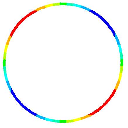
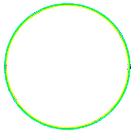
Figure 4.4 – Shear Stress and von Mises Stress Distribution in Burst Test (Case 1)

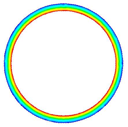
Figure 4.5 – Shear Stress and von Mises Stress Distribution in Collapse Test (Case 6)

With respect to cases 11-15, the maximum stress achieved was present at the inner maximum diameter, as shown in Figure 4.6. As the tests performed were designed to calculate parameter values at the first instance of failure, this resulted in only a small section of the model reaching the design limit meaning the majority of the model was far from reaching this point of failure, which may possibly result in innacuracies when determining the correct collapse pressure. This in turn means that the values achieved were very conservative with respect to failure of the complete model. This being said, although the maximum pressure likely could achieve a much larger value; due to the safety risk, the model will be said to have failed at the first instance of any element exceeding the design stress.

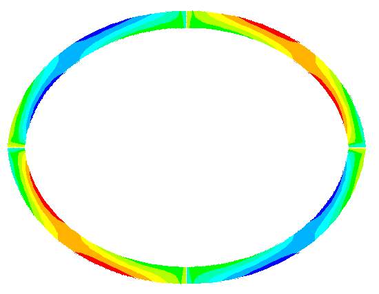
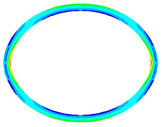
Figure 4.6 – Shear Stress and von Mises Stress Distribution in Collapse with Ovality Test (Case 11)

5. Results of Finite Element Model Simulation

As mentioned previously in the theoretical solutions, most pipeline codes around the world limit the design stress to 72% of the specified minimum yield stress (SMYS). For the API 5L X65 material used in the finite element model tests, the SMYS is equal to 450MPa and so, the design stress is roughly 324MPa. Therefore, this is the resultant stress we will be aiming to achieve in the simulations to correctly validate the ‘parameter relationships to prevent failure’ presented in Figures 3.1, 3.2 and 3.3.

5.1 Validation

The following scatter plots, Figures 5.1, 5.2 and 5.3, show the maximum value of von Mises stress achieved for each case study, with an indication of the proximity to the SMYS (450MPa) – the point at which plastic deformation begins – labelled on the plot as ‘Failure Line’.

Tables 5.1, 5.2 and 5.3 show the results for cases 1-15. The von Mises stress is taken as the maximum achieved stress present anywhere in the model, and the design stress is 72% of the SMYS. The error represents the difference between the two as compared with the original design stress.

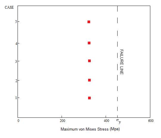
Figure 5.1 – Maximum von Mises Stress Achieved for Case 1-5

Case Study	von Mises Stress (Mpa)	Yield Stress (Mpa)	Design Stress (Mpa)	Error (%)	Results
1	328	450	324	1.23	ok
2	328	450	324	1.23	ok
3	327	450	324	0.93	ok
4	328	450	324	1.23	ok
5	327	450	324	0.93	ok

Table 5.1 – Error Percentage of Achieved Stress to Design Stress for Case 1-5

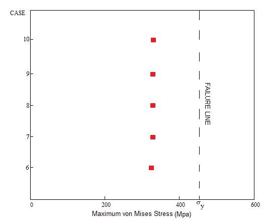
Figure 5.2 – Maximum von Mises Stress Achieved for Case 6-10

Case Study	von Mises Stress (Mpa)	Yield Stress (Mpa)	Design Stress (Mpa)	Error (%)	Results
6	328	450	324	1.23	ok
7	332	450	324	2.47	ok
8	332	450	324	2.47	ok
9	334	450	324	3.09	ok
10	335	450	324	3.4	ok

Table 5.2 – Error Percentage of Achieved Stress to Design Stress for Case 6-10

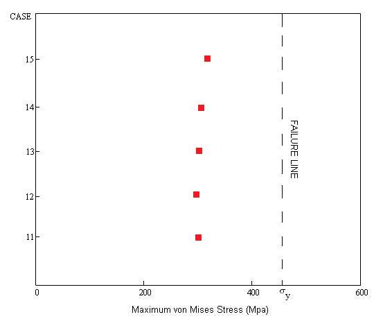
Figure 5.3 – Maximum von Mises Stress Achieved for Case 11-15

Case Study	von Mises Stress (Mpa)	Yield Stress (Mpa)	Design Stress (Mpa)	Error (%)	Results
11	301	450	324	-7.1	ok
12	298	450	324	-8.02	ok
13	312	450	324	-3.7	ok
14	314	450	324	-3.09	ok
15	328	450	324	1.23	ok

Table 5.3 – Error Percentage of Achieved Stress to Design Stress for Case 11-15

The results were all accurate on average to values of 98.9% for Burst tests, 97.5% for Collapse tests, and 96% for Collapse with an Initial Ovality tests. For Tables 5.1 and 5.2, design stress values were on average 73.3% of the SMYS which is acceptable for the scope of this work – to prove the most influential parameter relationships in order to prevent failure of the pipeline and thus, the weighting of each factor. For Table 5.3, design stress was recorded at an average of 69% SMYS, which again prove the calculated values of collapse pressure are fairly conservative. Notably, the largest error percent is for case 11 and 12 which correspond to 2% and 4% ovality, and as seen from the relationship in Figure 3.3 this is where values of collapse pressures plummet, hence, a very slight inaccuracy may be expected.

6. Conclusion

All of the most influential parameters and their relationships whith each other in order to prevent the burst or collapse behaviour of marine pipelines were proven to be correct to an acceptably accurate standard by ANSYS Mechanical version 16.0.

Thereby, having this information readily available to an acceptable standard will allow engineers when considering pipeline design to use the information provided in Figures 3.1, 3.2 and 3.3 and apply these basic principles with confidence.

6.1 Key Findings

From Figure 3.1, it can be observed that the maximum internal operating pressure can be increased by up to 29% for each 500m of water depth, with respect to the API 5L X65 material with an initial internal pressure of 17388kPa. This being said, using internal pressure to restore equilibrium due to extreme hydrostatic pressures may be a dangerous way of saving money by keeping diameter to thickness ratio constant. For example, if the internal pressure were ever to drop below the calculated value, the pipeline would be susceptible to collapse behaviour and therefore, this method should only be used if internal pressure can be guaranteed to stay constant throughout operation.

Secondly, the results from Figure 3.2 show that the diameter to thickness ratio is less affected at higher external pressures, and the main concern is in the initial first drop of 500m water depth. For example, the API 5L X65 material must reduce the diameter to thickness ratio from 64.2 to 42.8 (30% decrease) between 1000m and 1500m water depth whereas, the ratio only drops from 25.7 to 21.4 (16.7% decrease) between 2500m and 3000m water depth, respectively.

Furthermore, the results concerning collapse pressure due to ovality presented in Figure 3.3 show that the mechanical behaviour of steel is extremely sensitive to ovality, as you can observe from the large drop in collapse pressure. This relationship shows that for a 2% ovality the collapse pressure more than halves from that with a perfectly round circumference. Furthermore, for a 2% ovality in the pipeline cross-section, and using the diameter to thickness ratio provided to prevent collapse at 3000m for a perfectly round circumference, the recorded maximum water depth in which the pipeline could operate was said to be 521m – which proves that for engineers looking to expand the reach of offshore facilities into depths of up to 3000m; keeping careful monitor of pipeline ovality is extremely important.

Lastly, in each of the mentioned relationships, a reference to the performance of titanium (Ti6Al4V) has been given to show a comparison between the most commonly used steels and titanium used in the offshore industry. It is seen that titanium outperforms steel in each of the tests carried out, yet is still far less widespread in the industry which leaves room for discussion. This means consideration into future work must be given in order to give an accurate comparison.

6.2 Future Work

So far, the work carried out in this report covers the basic mechanical strength tests required to understand the weighting of each influencial parameter on the behaviour of marine pipelines. However, this may not be enough to fully comprehend the performance of materials in an offshore environment, and with further evaluation it may be possible to learn if introducing ‘newer’ materials may give a higher performance overall when reaching out into water depths of up to 3000m.

To give an improved comparison between the benefits of materials over one another, further research may be needed in areas such as fatigue, toughness, manufacturing, installation and environmental conditions. For example, this may cover topics such as a materials resistance to corrosion due to the flow of crude oil or the marine environment; the weldability of pipeline materials and also of one component to another i.e. the difficulties in welding a pipeline with a 2% ovality imperfection to one with a perfectly circular cross section; the economical considerations when manufacturing, such as the cost per material versus it’s weight and strength capabilities; and the weight gain potential of newer materials such as composites – either thermosetting or thermoplastic, which could be endless with regards to installation.

From gaining a fuller understanding of the contribution and influence that each of these factors have on the long term durability of materials, we may be able to understand if there is potential for ‘new’ materials to make their way into the industry as a substitute for steel. These may include titanium – which we have looked at briefly and shows great signs for potential, and also materials such as aluminium and advanced composites.

Furthermore, on having reliable and accurate performance data on a selection of materials, it would give the potential to apply this to a variety of offshore applications. So far the work in this project, and the future work described previously in this chapter, only applies to fixed (rigid) marine pipelines however, with having the principal rules and relationships between parameters readily available it may be possible to study a range of subsea equipment, such as flexible pipelines and rigid and flexible marine risers, with more ease since we now have the tools to accurately determine the performance of one material over another in terms of durability, safety and economic viability.

Bibliography

American Petroleoum Institute (1999) ‘API Recommended Practice 1111’ Third Edition

Assarar M, Scida D, El Mahi A, Poilane C, Ayad R (2011) ‘Influence of water aging on mechanical properties and damage events of two reinforced composite materials: flax fibres and glass fibres’, Materials and Design, 32, 788–795.

Corona E, Kyriakides S (1998) ‘The collapse of inelastic tubes under combined bending and pressure’ Int J Solids Struct, pp. 24:505-35

Davies P (2016) ‘Marine Applications of Advanced Fibre-Reinforced Composites.’ Edited by J. Graham-Jones, J. Summerscales. Woodhead Publishing, pp. 125-145, 20160

Hine P J, Duckett R A, Kaddour A S, Hinton M J, Wells G M (2005) ‘The effect of hydrostatic pressure on the mechanical properties of glass fibre/epoxy unidirectional composites.’ pp. 279-289

Kaviti R V P, Bhimasankara T (2013) ‘Ovality in Pipe Bends by Finite Element Analysis’ International Journal of Engineering Research and Development, Vol.6 Issues 5, pp. 91-97

Lange H, Berge S (2004) ‘Material Selection in the Offshore Industry’ NPDS SINTEF Report

Pauchard V, Grosjean F, Campion-Boulharts H, Chateauminois A (2002) ‘Application of a stress corrosion cracking model to the analysis of the durability of glass/epoxy composites in wet environments’, Composites Science and Technology, 62, 493–498.

Pharris T C, Kolpa R L (2007) ‘Overview of the Design, Construction, and Operation of Interstate Liquid Petroleum Pipelines’ Environmental Science Devision, Argonne National Laboratory

Salama M, Storhaug T, Martinussen E, Lindefjeld O (2000) ‘Application and remaining challenges of advanced composites for water depth sensitive systems’, paper presented at Deep Offshore Technology Conference, 2000.

Sung J M (2012) ‘Anisotropy of Charpy Properties in Linepipe Steels’ Doctoral Thesis’ Department of Ferrous Technology, Pohang University of Science and Technology

Timoshenko S P, Gere J M (1961) ‘Theory of Elastic Stability.’ New York, McGraw-Hill

Toscano R G (2009) ‘Collapse and post-collapse behaviour of steel pipes under external pressure and bending. Application to deep water pipelines’ Doctoral Thesis, Universidad de Buenos Aires

Vodar B, Kieffer J (1971) ‘Historical Introduction, the Mechanical Behavior of Materials Under Pressure.’ Edited by H.L.D. Pugh. London: Applied Science Publishers, Ltd., pp. 1-53, 1971

Wu P D, Embury J D, Lloyd D J, Huang Y, Neale K W (2009) ‘Effects of superimposed hydrostatic pressure on sheet metal formability.’ International Journal of Plasticity, pp. 1711-1725

Yang Y, Khana F, Thodi P, Abbassi R (2017) ‘Corrosion induced failure analysis of subsea pipelines.’ Reliability Engineering and System Safety 2017

Zhang J, Nash K, Arrigoni A, Escobedo J P, Florando J N, Field D P (2017) ‘Materials Science and Engineering.’ A, Volume 679, pp. 155-161