ABSTRACT

This paper is concerned with the influence of mesh quality on the finite element analysis of geotechnical problems. It studies the relationship between mesh quality and accuracy of results produced. Finite element method (FEM) is commonly used for the analyses of geotechnical problems such as the bearing capacity of foundation(Potts and Zdravković, 2001). In this study, vertical behaviour (such as the load-displacement relationship) of a strip footing will be analysed due to the change in mesh quality by means of a FE model.

For a successful finite element analysis (FEA) of a geotechnical problem, a constitutive soil model is necessary. Finite element method is useful for numerical modelling of appropriate soil bodies. (Md Nujid and Raihan Taha Professor, 2014). The soil in the model is subdivided into elements by meshing it. Mesh sizing is very critical and relates closely to the accuracy. It is eminent that the numerical results depend largely on the complexity of the model and number of elements involved in the analysis. With more elements, computational time also increases. (T. More and Bindu, 2008). The software ABAQUS is chosen to investigate the various effects of the change of parameters on the soil, and to optimise a mesh suitable for Finite Element Analysis.

Results obtained from the simulation of the FE model will then be validated by correlating them to either laboratory experiment data or existing solutions from literature review. Any differences observed will be discussed. The results will then be used to find the perfect mesh size for the finite element analysis.

TABLE OF CONTENTS

Click to expand Table of Contents

CHAPTER 1: INTRODUCTION

1.1 BACKGROUND

1.2 OBJECTIVE AND SCOPE

CHAPTER 2: LITERATURE REVIEW

2.1 FOUNDATIONS

2.1.1 BEARING CAPACITY

2.1.1.1 DRAINED LOADING

2.1.1.2 UNDRAINED LOADING

2.2 EXAMPLE

2.2.1 STRIP FOOTING UNDER VERTICAL LOADING ON UNDRAINED CLAY

CHAPTER 3: FINITE ELEMENT ANALYSIS

3.1 FINITE ELEMENT METHOD

3.2 ABAQUS SOFTWARE

3.3 WORK UNDERTAKEN

3.3.1 BRIEF OVERVIEW

3.3.2 DETAILS OF THE MODELLED ANALYSIS

CHAPTER 4: RESULTS AND DISCUSSIONS

4.1 DISCUSSION

4.2 ERRORS AND LIMITATIONS

CHAPTER 5: CONCLUSION

5.1 SUMMARY

5.2 RECOMMENDATION FOR FURTHER WORK

REFERENCES

APPENDIX

CHAPTER 1: INTRODUCTION

1.1 BACKGROUND

The Finite Element Method (FEM) is a numerical method for solving problems with complex geometries, loading and material properties. It is commonly used in analysis of geotechnical problems to obtain approximate solutions of boundary value problems. The FEM is also known as the Finite Element Analysis (FEA), where large and complex problems are discretised into smaller, more manageable parts called the Finite Elements (FE). Different parameters are specified and behaviour of these finite elements are simulated and analysed under a variety of conditions.

The mesh size plays a vital role in the accuracy of results and computing time as it determines the number elements involved.; According to the FEA theories FE models with coarse mesh yields less accurate results and has a reasonably small computing time. A coarse mesh means that there are less number of elements present and that these elements will have a large element size. Coarse mesh is more suitable for problems where quick and rough estimation of design is required. On the other hand, finer mesh is used in problems that require high accuracy. Finer mesh means smaller element size and thus requiring a longer computing time due to the large number of elements involved, hence making it more expensive.

The finite element method is used in this study to analyse a vertically loaded strip footing on soil (which may either be drained or undrained). A strip footing is a component of shallow foundation, it is a continuous strip of concrete that supports the weight of the whole wall across the area of soil in consideration. As per conventional foundation design, the Mohr-Coulomb failure criteria is used to define the plasticity of the soil. Accuracy of the results are investigated through modelling laboratory experiments and comparing with any existing data from literature review.

1.2 OBJECTIVE AND SCOPE

The objective of this paper is to study the influence of mesh size on the vertical loading behaviour of a strip footing and provide guidelines to select the optimal mesh size for different finite element analyses. In this study, the bearing capacity analysed using ABAQUS. Boundary conditions will be defied and loads will be applied to the model and corresponding stress, strain and deformations can be obtained from the analysis. The strip footing on the model will be a rigid body so no deformation will be there due to the vertical loading. The analysis will be run several times using FE models of varying mesh sizes in each of the simulations. The penetration of the strip footing into the soil will be observed and recorded. Bearing capacity of the foundation will then be analysed. This is done to show the effects on stress and displacement as the mesh sizes are varied. This helps achieve the optimal combination of accuracy of results and efficiency of the analysis.

A certain amount of error will be present in the solutions produced by the finite element analysis depending on the size, type and accuracy of the model used relying on the availability of appropriate soil data. To minimise this, validation of the model is compared to the results obtained by other measured tests or any existing results obtained from the literature review.

CHAPTER 2: LITERATURE REVIEW

2.1 FOUNDATIONS

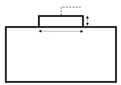
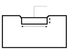
Foundations are an essential part of a geotechnical structure. It allows the loads from the structure to be transferred into the soil. The type of foundation is determined on the basis of the depth of the soil in which it is constructed. There are two main types of foundation, shallow foundation and deep foundation. Deep foundations include basements, caissons, shafts and piles. They are usually built at depths that are greater than 3m while Shallow foundations are used for depths of 1.5 m. they are usually strong enough to support the structural loads imposed on them. The ratio of the embedment depth of these shallow foundations to their width is usually less than 3 (D/B<3). Shallow foundations include spread footings, strip footings, mat foundation and raft foundation. In this paper the bearing capacity of a strip footing will be looked at. A strip footing is a component of shallow foundation. They are used in case of a load bearing wall to evenly spread out the loads applied on the wall to the ground. It is also used when a row of columns is placed close to each other and their spread footings almost touch one another. Therefore, instead of placing each spread footing individually it appears to be more economical to provide a strip footing. Strip footing also goes by the name continuous footing. The strip footing and soil interaction can be simply illustrated in figure 1. A strip footing having width of B and depth of D is placed on top of a soil model which then slowly embeds shallowly.

           

Strip Footing

Strip Footing

D

B

D

B

Soil model

Soil model

Figure 1 Schematic of strip footing and soil interaction as it slowly embeds.

2.1.1 BEARING CAPACITY

Bearing capacity (q) is defined as the maximum bearing stress of the soil to support the loads that are imposed on the structure after which shear failure occurs in the soil. The ultimate bearing capacity (q_ult) causes settlement due to the shear failure. To ensure that the foundation is stable and that settlement is tolerable, the bearing pressure needs to be within allowable limits. The allowable bearing capacity can be calculated using a Factor of Safety (Fs) with the ultimate bearing capacity.

The expression proposed by Karl Von Terzaghi is generally used to estimate the bearing capacity of shallow foundation (under both drained and undrained loading (Terzaghi, 1943). The equation is as follows:

= c _c + _{0 q} + 0.5

Where, q = the ultimate bearing capacity (q_ult). c = the cohesion intercept. 0 = the total stress at the level of the base of the foundation. B = the width of the footing. = the bearing capacity factor that represents the contribution of cohesion of soil. = the bearing capacity factor that represents the contribution of surcharge to the overall bearing capacity. = the bearing capacity factor that represents the contribution of soil self-weight.

Some of the Assumptions Terzaghi used in his analysis were that the strip footing was at a shallow depth with a rough base and that the length, L was greater than five times its width, B (L>5B) and that the depth, D was greater than its width, B (D > B). The soil was assumed to be homogenous and comparatively incompressible. The failure zones were expected not to spread above the horizontal plane over the footing’s base. Lastly, the elastic zone was thought to have straight boundaries with an inclination of џ = φ to the horizontal and the plastic zones being developed fully.

The equation was later attempted to be improved using shape factors S_c and S_y. When restrictions were discovered. For strip footings both S_c =1.0 and S_y =1.0. Therefore, a shallow strip foundation having with B and depth D, will have the following equation for the bearing capacity:

= (c _cS_c) + ( _{0 q}) + (0.5 S_y)

= (c _c (1.0)) + ( _{0 q}) + (0.5 (1.0))

= (c _c) + ( _{0 q}) + (0.5 )

2.1.1.1 Drained loading

The equation used for the ultimate bearing capacity of a strip footing under drained loading is shown below:

= ( ₀ ) + (0.5 )

Where, q = ultimate bearing capacity (q_ult). 0 = the total stress at the level of the base of the foundation. B = the width of the footing. = bearing capacity factor that represents the contribution of surcharge to the overall bearing capacity. = bearing capacity factor that represents the contribution of soil self-weight.

The position of water table is essential. The groundwater level influences the effective stresses that are used in the analysis for drained loading of a shallow foundation. Both shear strength and effective stress of the soil is affected by shallow groundwater. They decrease while pore pressure on the other hand increases. If the water table is located below the strip footing’s base, then water will not have any effect on the ultimate bearing capacity. The values of and can be obtained from the following graph as shown in figure 2. Figure 2 plots the values of and against the soil friction angle.

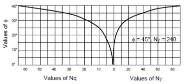
Figure 2 Bearing capacity factors N_q, N_y (after Terzaghi and Peak, 1967)

2.1.1.2 Undrained loading

The equation used for the ultimate bearing capacity of a strip footing on a saturated undrained clay is shown below in equation. For an undrained analysis, the total stresses are used. The cohesion intercept of the undrained clay is equal to its undrained shear strength, Su and the effective stress friction angle, φ’ is zero.

= c _c + _{0 q}

= × + 0

Where, q = ultimate bearing capacity (q_ult). = the undrained shear strength, c = bearing capacity factor that represents the contribution of cohesion of soil. It depends on the shape and depth of the foundation. 0 = the total stress at the level of the base of the foundation.

For a strip footing on the surface, Prandtl (1921) used the plasticity theory to determine the bearing capacity factor N_c to be 5.1416.

The bearing capacity factor, N_c in Terzaghi’s equation seems to increase with the increase in depth for a cohesive soil. (‘Module 4 : Design of Shallow Foundations’). This is demonstrated by Skempton in the following figure 3. The figure shows that a strip footing at ground level has depth to width ratio, D/B = 0 and therefore the N_c value is (2+ ) = 5.1416, while =1 and =0 (Skempton, 1951).

Figure 3 also shows the transition of bearing capacity from shallow to deep for soil that is uniform throughout and beyond depth D and has a uniform strength Su.

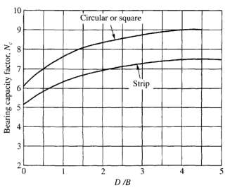
Figure 3 Skempton’s bearing capacity factor Nc for clay soils

2.2 EXAMPLE

Literature review of the ultimate bearing capacity of a shallow foundation under vertical loading is presented with emphasis on strip footings. A scenario is analysed where a non-uniform mesh is used. A strip footing is vertically loaded on an undrained clay The undrained clay is modelled by means of linear elastic Tresca model. This is done to be consistent with conventional design of foundation. Result obtained in the analyses are compared to the solutions of conventional bearing capacity(Potts and Zdravković, 2001).

2.3.1 Strip footing under vertical loading on undrained clay

In order to obtain the load-displacement curves for rigid strip surface footings, analyses are performed. Elasto-plastic soil with Tresca yield surface and the following properties were considered. The soil had a Young’s Modulus, E of 100 MPa, a Poisson’s Ratio of 0.49 and an undrained strength, S_u of 100 KPa.

The kind of mesh used is uniform around the strip footing. As it goes further away the mesh gradually becomes non-uniform as shown in the figure 3:

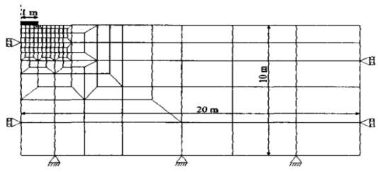
Figure 4 Finite element mesh for strip footing analysis.

Boundary conditions have been applied to the soil, where the two sides of the mesh have been restricted in the horizontal direction. While the bottom layer has been made fixed. It is restricted in both horizontal and vertical direction. Increments of the vertical displacement are applied to the surface of the soil below the position of the footing as loads are simulated. As the strip footing penetrates the soil, displacement is recorded. The load against displacement curve is shown below:

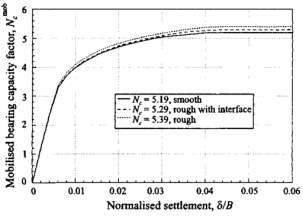
Figure 5 Load-Displacement curves for (smooth, rough with interface and rough) strip footing.

The bearing capacity of a strip footing loaded vertically on undrained clay is usually expressed as:

Q_max = A N_C S_U

Where,Q_max = Maximum vertical load applied to the footing. A = Area of the footing. N_C = Bearing capacity factor. S_U = Undrained strength.

The load is expressed in terms of mobilized bearing capacity factor, N_C ^mob in Figure 4.

N_C = =

QASu

The displacement is distributed by B.

Settlement = =

δB

Where,

δ= displacement and B = half width of the footing

Figure 4 shows results from three analyses modelled. One is a smooth footing while the other two are rough. Interface elements were added between the soil and the footing in one out of the two rough ones. This is illustrated in the figure 6:

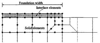
Figure 6: detail of mesh with interface elements

A shear strength of 100 KPa and shear and normal stiffness of value, K_s = K_n = 10⁵kN/m³ were given to the interface elements. It can be seen on figure 5, that different load-displacement curves and N_c values were produced for the three analyses.

The theory of conventional bearing capacity indicates that the bearing capacity factor, N_c for both smooth and rough footing should be the same as (2+π) = 5.1416 (Prandtl, 1920). The value is theoretically exact and can be obtained from limit analysis and a closed form plasticity solution. By comparing the results obtained from the finite element analysis and the analytical solution, it is seen that the results differ by 0.94%, 4.6%, 2.8% for the smooth (N_c =5.19), rough (N_c =5.39) and rough with interface element (N_c =5.29) respectively.

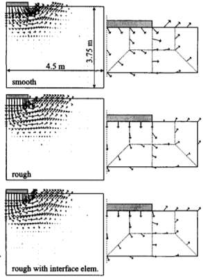
Figure 7: Vectors of incremental displacements at failure for three different soil-footing interfaces.

Figure 7 shows the vectors of incremental displacement at failure which is the last increment of each analysis. The direction of movement is indicated by the orientation of these vectors and magnitude of the movement by the length. The failure mechanism is indicated by the orientation and the relative magnitude of the vectors. The failure mechanisms indicate some movement in the horizontal direction at the surface of the soil under the smooth footing. However due to boundary condition of the rough footings, they are not allowed to move so the failure mechanisms are a little deeper and wider in comparison. A bigger ultimate footing load and N_c is obtained due to the larger slip surface area, A which is then combined with S_u.

The nature of finite element mesh below and adjacent the footing may contribute to the errors. As per figure 7 it is seen that the direction of displacement vectors next to the edge of the rough footing change abruptly from going vertical downwards at an angle of 45° under the footing corner to horizontal in an upward path next to the footing on the soil surface. This happens over the single element that is located at the corner. Ability of this single element to put up with the rapid change of displacement will determine the accuracy of the results. To obtain accurate solutions, a finer mesh needs to be used. This means that the element sizes should be made even smaller around the edge of the footing. Due to this singularity at the edge of the footing, computation time becomes larger. Nonetheless, more accurate results could be obtained with the help of a refined mesh. To increase accuracy of the results further, the overall mesh size throughout the model can be made smaller instead of just the ones near the corner.

CHAPTER 3: FINITE ELEMENT ANALYSIS

3.1 FINITE ELEMENT METHOD

The Finite Element Analysis (FEA) is the implementation of the Finite Element Method (FEM) that is used to solve certain problems. The Finite Element Method is a numerical method used to solve partial differential equations with boundary conditions by using multiple sub functions in a polynomial interpolation.(WELCOME TO ENGINEERS CADD CENTRE (P) LTD). This method draws out the shape of the original differential equation curve with the help of several polynomial curve shapes in order to simplify the more complex curve. This method is helpful for problems with complicated shapes, loadings, material properties etc. (‘Introduction to Finite Element Analysis (FEA) or Finite Element Method (FEM)’). The intervals are then evaluated with respect to the points that encloses that section of the polynomial curve. The FEA solutions are then evaluated and the results (such as deflection and stress) are only given at these points called nodes. ­

According to the documentation of Abaqus (2010), it is important to discretize the geometry of a structure into finite element before any finite element simulation is run. Therefore, the structure that will be analysed is subdivided in a mesh of finite elements, breaking down the original shape of the structure or the object into simpler shapes. The finite elements are connected to each other by their nodes. The nodes are a coordinate location which define the degrees of freedom (DOFs) in space. The movement of these points under loading of the structure is represented by the degrees of freedom. They also represent the forces and moments that are being transferred to the next element. The finite elements and the nodes collectively form up the mesh.

It is assumed that the simple polynomial curve shapes and the nodal displacements determine the change in displacement of each of these elements. Stress and strain equations are constructed with respect to the unknown nodal displacements. The equations of equilibrium are then assembled in the form of a matrix so that they can be programmed and solved. After suitable boundary conditions are applied, the stiffness matrix equation can then be solved in order to find nodal displacements. The element stresses and strains can easily be calculated once the nodal displacements are obtained.

3.2 ABAQUS software

Abaqus is a general-purpose simulation software used in different engineering fields and is based on finite element method. It has a graphical user interface to pre-process the input files and post process the results. A lot of literature reviews suggest that Abaqus is frequently used to solve several geotechnical problems. An example of the features which make this software popular to use is the availability of the Mohr-Coulomb yield criteria application. The Mohr – Coulomb yield criterion is frequently used for defining the elasticity of soils in finite element method (Hasan Emre Oktay, 2012). Abaqus is chosen as the software to be used for the finite element analysis due to its several advantages.

Numerous ways of modelling and multiple choices of algorithms are offered to find solutions of the modelled problem. A number of powerful mesh generating algorithms can be inserted into each of the modelling schemes. These algorithms (functions) will then determine whether the system will behave in a linear or a non-linear manner. Non-linear systems are more complex when compared to the linear systems. Linear systems usually ignore a few restraints of the model such as loading and behaviour. Non-linear systems on the other hand take more realistic behaviour of the model such as plastic deformation, varying loads etc. into consideration. This allows it to test the model up to its failure. Having said that, for any method chosen, it consists of many predefined formulations for elements and material models which can produce acceptable results.

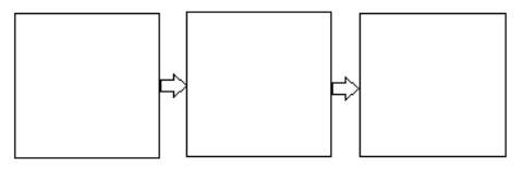
Abaqus supports scripting functionality and command line can be accessed. It allows the user to create a very detailed model. In addition, it can solve problems that behave in both linear and nonlinear fashion and it can conduct 2D as well as 3D analyses. Furthermore, software license is easily available making it more desirable to use. Three simple steps used in the software are shown in figure 8.

An ASCII text file is required as an input for the Abaqus analysis product, Abaqus/Standard. All aspects of the model such as the coordinates of the nodes, analysis steps and requested output variables are held by this file. This file can be either created manually from scratch, or edited using an existing file. The Abaqus CAE pre-processor software can also be used. The Abaqus CAE uses a graphical user interface for them to create, edit monitor, diagnose and visualize advanced analysis. It is usually very user friendly for beginners. Most of the features of Abaqus can be utilized from the Abaqus CAE. However, input files will be used instead of Abaqus CAE in this study. Abaqus CAE can either store modifications or the input files can be modified manually. Certain variable value of selected entities can be saved by Abaqus as an output. The state of a complete model for a certain variable can also be recorded. Before it was called the history output request but now it has been changed to field output request as per Abaqus documentation of 2010. The requests are written to an output database file. The binary format of the file can be read by Abaqus CAE. Forms of other output formats exist, where history output can be saved in either ASCII file formats or in binary that can be opened by third party software.

Evaluation and simulation

Abaqus/standard or

Abaqus/explicit

Post-processing (visualization)

Abaqus/CAE or other products

Pre-processing

(Modelling)

Abaqus/CAE or other products

Figure 8: Simple tests of Abaqus

3.3 WORK UNDERTAKEN

3.3.1 Brief overview

To design the Finite Element model of the soil for the strip footing, the geometric domain of the problem needs to be defined along with the element type, material and geometrical properties like the length, area etc. The model can then be meshed using variable mesh sizes in each simulation to determine the element size that is most suitable. Lastly, the boundary conditions will be applied. After the model is created, the simulations will be run and analysed. The results obtained will then be compared to existing solutions from literature review and other laboratory experiment data (if available). By doing this the effects of mesh sizing on the bearing capacity of the strip footing can be found.

3.3.2 Details of the modelled analysis

The type of soil chosen for the analysis was an undrained soil having a density of 0.1 kg/m³. Young’s modulus of 400×10⁹ Pa and a Poisson’s ratio of 0.495 was assigned to the finite element soil model. The dimension of the soil model was 10m long with a height of 5m. The breadth of the model varied with the size of the mesh for each simulation (for example, 0.2m, 0.1m, 0.05m etc.). A 2m long strip footing model was placed at the centre of the surface of the soil model. The strip footing had a rectangular shape with a height of 0.5m and breadth of 0.2m. The surface of the soil interacting with the base of the strip footing was made rough by setting the cohesion factor, α as 1. This means that the friction was equal to the normal force. The three-dimensional soil model was constructed using an input file and then it was imported into the ABAQUS software. The explicit dynamic finite element module was then used for the analysis.

It was seen that the finite element model could be established using both the ABAQUS CAE and by writing input files based on previous sample work. Based on the conclusion that both files produced same results, input files were chosen to create the FE model to make the process time efficient.

Three finite element models were generated for the soil with mesh size of 0.20m, 0.10m and 0.05m using input files. A sample input file has been attached as appendix. In the input files, the model was divided into two different bodies, a sea-bed and a rigid strip footing. The material for the sea-bed is chosen to be a eulerian material. The coordinates of the sea-bed are defined and the node numbers are assigned. The whole domain is then divided and grouped into node sets (Nset). The nodes on the top and bottom are grouped and named ‘Bottomtop’. The nodes on the left side of the model are grouped and ‘Left’. The nodes on the right side of the model are grouped named ‘Right’. A few more node sets were defined. Similarly, the sea-bed, the void on top of the surface and the pipe (the strip footing) were generated by allocating the node numbers and were grouped into element sets (Elset).

The coordinates of the strip footing were then defined and node numbers were assigned just like the sea-bed. It can be seen on the input files that the node numbers of the strip footing are listed under the heading ‘node’ along with their coordinates. The element numbers for the strip footing is also shown under the heading ‘element’ along with the number of nodes that make up the element. The type of element chosen for the strip footing is the R3D4. This shows that the element is a 3D rigid quadrilateral element. The reference point for the strip footing was set by specifying the node number. After creating the FE model, the material of the sea-bed needs to be assigned. As mentioned earlier, an undrained soil is selected. Apart from the density, young’s modulus, Poisson’s ratio, the cohesion yield stress of the soil is assigned as 1. After assigning all of them in element sets, the boundary conditions are applied. It is usually easier to change parameters or apply boundary conditions to a collection of nodes or elements rather than applying them to each individual node or element. This process can become very difficult and time consuming. In these situations, it is helpful to break down the FE model into smaller sets, making the process much simpler and time saving.

The strip footing did not experience any deformation while it penetrated since it was modelled as a rigid body. The soil was modelled to have a homogenous shear strength all over the model. The edge on the right side was restrained in both vertical and horizontal direction thus making it a fixed end. Similarly, the bottom of the soil domain was also made fixed. Symmetry boundary conditions were assigned to the left edge. This is because It was assumed that the model was symmetrical about the plane normal to the center of the strip footing. Therefore, only the right half of the arrangement was modelled and analysed. The plane of symmetry is shown by the symmetry line in the x-z plane in Figure 9. The strip footing moved in the vertical direction in the downward y plane as it settled.

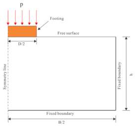
Figure 9 Half of the arrangement to be analysed

CHAPTER 4: RESULTS AND DISCUSSIONS

4.1 DISCUSSION

The results of the analysis will be shown and discussed in detail in this chapter. The main objective is to describe the influence of mesh quality on the bearing capacity of the strip footing based on the results obtained from the finite element analysis. Results obtained from the Finite Element Analysis are put into graphical solution so that they can be compared directly. These results are compared among each other and then compared with the analytical value obtained from literature review to see which mesh has the most suitable results.

The outcome of the three input files are shown in this chapter. The figures 9, 10 and 11 show the finite element model with the mesh sizes 0.02m, 0.10m and 0.05m respectively. The strip footing is represented by the red box. The sea-bed is represented by the blue box and the void above the sea-bed is respresented by the purple box.

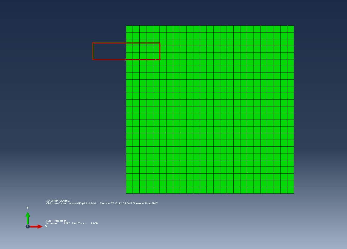
Figure 10 Finite element model with mesh size 0.20m

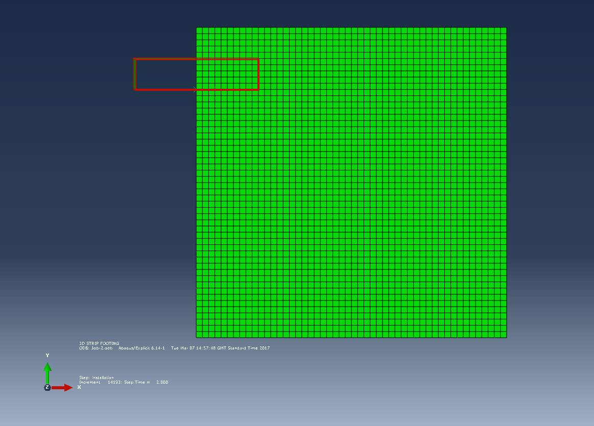
Figure 11 Finite element model with mesh size 0.10m

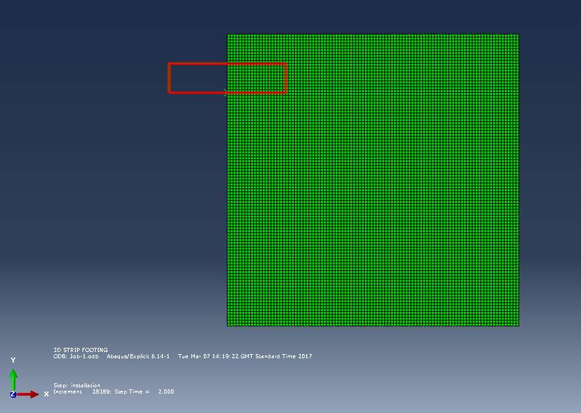
Figure 12 Finite element model with mesh size 0.05m

Analysis part 1

As the strip footing is embedded into the soil bed, the soil-bed undergoes displacement. The displacement increases linearly as the time increases. For all three meshes, the displacement was seen to be 0.1m vertically down for half of the model that was analysed. Figure 12 shows the shape of the displacement against time graph that was obtained for each of the meshes.

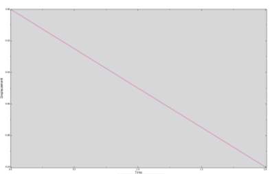
Figure 13 Displacement-Time graph for the mesh sizes of 0.20m, 0.10m and 0.05m

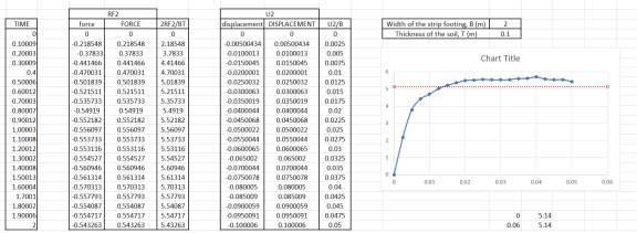
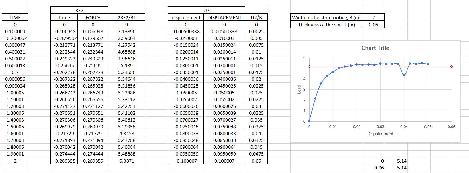
For each of the different mesh size, the load against displacement curves have been plotted in one graph along with the analytical value of N_c = (π+2) = 5.1416 suggested by Prandtl (Prandtl, 1920) for comparison. The set of values of Reaction force, RF2 and the set of values of Spatial displacement, U2 obtained from the analysis were processed to plot these curves. Since the model is symmetric, the force imposed had to be multiplied by 2. The raw data used for plotting these graphs are shown in the appendix. Figure 13 shows the Load against displacement curves for the three different mesh sizes.

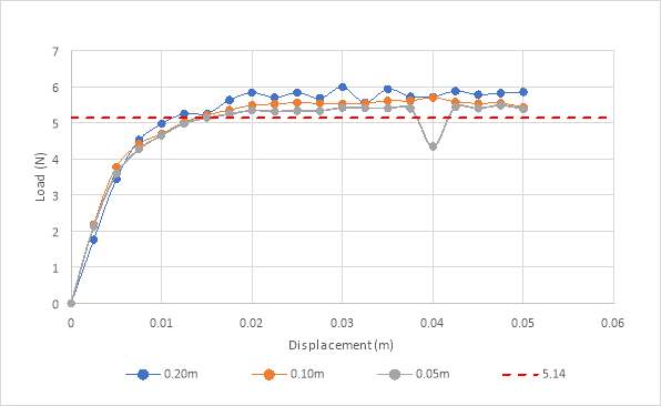
Figure 14 Load-Displacement graph for analysis part 1

From figure 14, it can be seen that the relationship between the load and displacement is a linear one. All the graphs increase in a straight line with increase in displacement. The rate of growth for the graphs eventually levelled off as the strip footing settled.

Average of 5 readings were taken to estimate the value at which they levelled out. The graph for the 0.20m mesh levelled out around 5.80 approximately.  The graph for the 0.10m mesh levels around 5.50 approximately and the graph for the 0.05m mesh levels around 5.37 approximately. The trend of these curves seems to be that the level at which they started to flatten out got closer and closer to the analytical value, 5.1416, with the more finer mesh. It was seen that the results varied by 12.81%, 6.97%, 4.44% for the 0.20m mesh (N_c =5.80), 0.10m mesh (N_c =5.50) and 0.05m (N_c =5.37) respectively. To reach the analytical value, even finer meshes need to be used.

The Von Mises stresses distribution on the soil due to the penetrating strip footing on the different mesh sizes are shown in figure 15, 16 and 17. Screenshots of the last time frame was taken for the three meshes so that the difference in stress at the end of the installation step could be seen properly.

Figure 15 Von mises stress distribution for 0.20m mesh

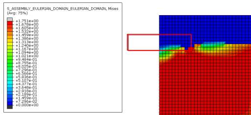
Figure 16 Von mises stress distribution for 0.10m mesh

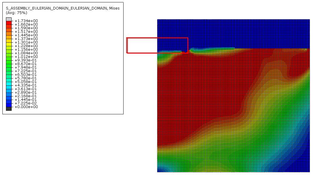
Figure 17 Von mises stress distribution for 0.05m mesh

Figure 15, 16 and 17 shows the von mises stress distribution on the finite element model. Screenshots of these stresses were taken on the last time frame to show the end of the installation stage of the settlement within the time specified. It can be seen that the stress is the highest near the corner of the footing for all three cases.

On figure 15, the stress near the corner is +1.733e+00 and occupies almost 3 elements, each having a width of 0.20m. On figure 16, the stress near the corner is 1.751e+00 and occupies 3 elements but this time each of their width being 0.10m. On figure 17, the stress near the corner is 1.734e+00 and occupies almost 5 elements but this time their width is even smaller, such as 0.05m. This shows that as the element size gets smaller, the element in the corner of the strip footing is able to distribute the load and put up will the change in displacement better than when it has larger sized elements.

Analysis part 2

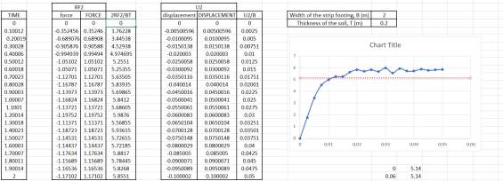
Further analyses were carried out to compare how the displacement is affected by the change in density of the soil, the density of the soil was changed from 0.1 kg/m³ to 0.2 kg/m³ . The load against displacement curves have been plotted together and shown in figure 18 along with the von mises stress distribution for the revised soil properties shown in figures 19, 20 and 21.

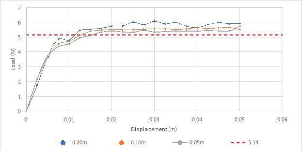
Figure 18 Load-Displacement graph for analysis part 2

After the density was changed from 0.1 kg/m³ to 0.2 kg/m³ , the load-displacement graphs obtained in figure 18, showed a similar trend to the graphs shown in figure 14. They too had a linear relationship. The curve starts off with a straight line that increased linearly and then eventually the growth decreased and they started to level out.

The graph for the 0.20m mesh levelled out around 5.80 approximately.  The graph for the 0.10m mesh levels around 5.53 approximately and the graph for the 0.05m mesh levels around 5.40 approximately. Again, the trend of these curves seemed to be that the level at which they started to flatten out got closer and closer to the analytical value, 5.1416, with the more finer mesh. It was seen that the results varied by 12.81%, 7.55%, 5.03% for the 0.20m mesh (N_c =5.80), 0.10m mesh (N_c =5.53) and 0.05m (N_c =5.40) respectively. To reach the analytical value, even finer meshes need to be used.

When compared to the results of figure 14, the results were quite similar. However, it was seen that the soil with lower density was closer to the analytical value rather than the one where the density was increased.

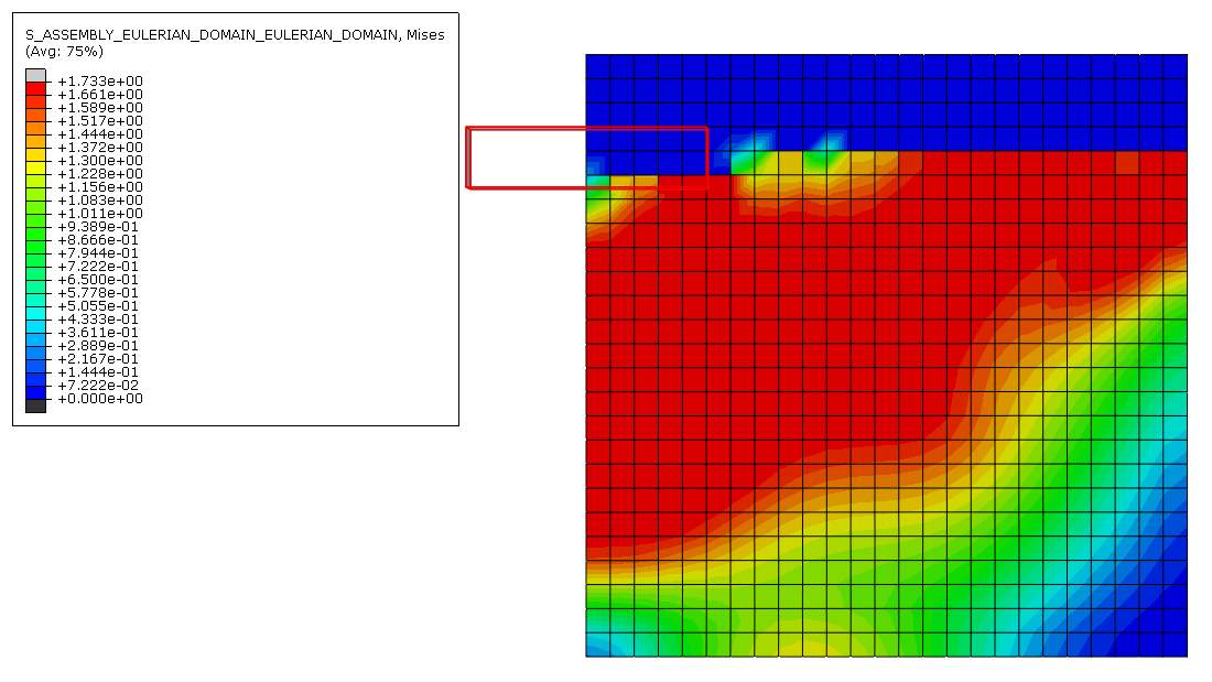
Figure 19 Von mises stress distribution for 0.20m mesh

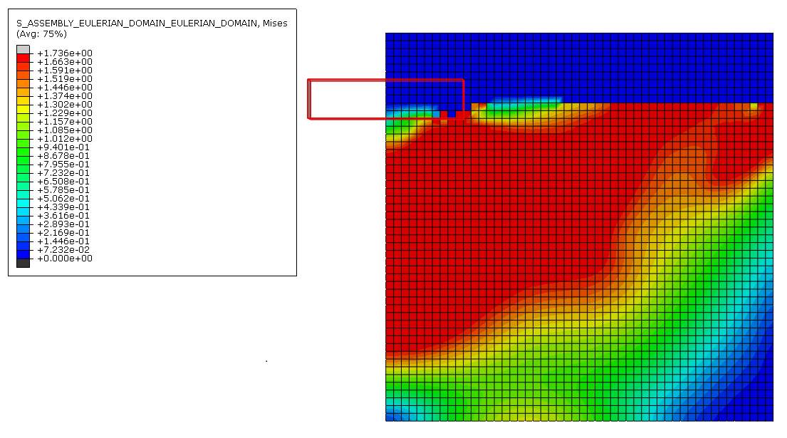
Figure 20 Von mises stress distribution for 0.10m mesh

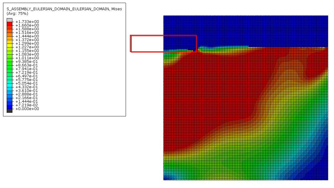
Figure 21 Von mises stress distribution for 0.05m mesh

Moving on to figure 19, 20 and 21. These figures show the von mises stress distribution on the finite element model with a higher density. Screenshots of these stresses were also taken on the last time frame to show the end of the installation stage of the settlement within the time specified. Once again, the stress is the highest near the corner of the footing for all three cases.

On figure 19, the stress near the corner is +1.733e+00 and occupies almost 3.5 elements this time, each having a width of 0.20m. On figure 20, the stress near the corner is 1.736e+00 and occupies around 5 elements, each of their width being 0.10m. On figure 21, the stress near the corner is 1.733e+00 and occupies about 6 elements, each of their width being 0.05m. This shows that as the element size gets smaller, the element in the corner of the strip footing is able to distribute the load and put up will the change in displacement better than when it has larger sized elements.

Analysis part 3

The loading rate was then changed in the input files by changing the original time in the installation step from 2s to 20s and the velocity was decreased from 0.05 m/s to 0.005 m/s to ensure that the total displacement was same for all the analyses. The load against displacement curves have been shown in figure 22, along with the von mises stress distribution in figures 23,24 and 25 for the revised loading rate.

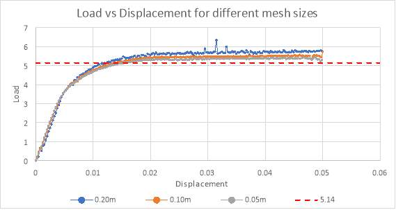
Figure 23 Load-Displacement graph for analysis part 3

After the time of the loading rate was changed from 2s to 20s and the velocity was changed from 0.05m/s to 0.005s, the load-displacement graphs obtained in figure 18, showed a similar trend to the graphs shown in figure 14 and figure 18. They too had a linear relationship. The curve starts off with a straight line that increased linearly and then eventually the growth decreased and they started to level out.

The graph for the 0.20m mesh levelled out around 5.72 approximately.  The graph for the 0.10m mesh levels around 5.44 approximately and the graph for the 0.05m mesh levels around 5.34 approximately. The trend of these curves seemed to be that the level at which they started to flatten out got closer and closer to the analytical value, 5.1416, with the more finer mesh just like the curves in figure 14 and figure 18. It was seen that the results varied by 11.25%, 5.80%, 3.86% for the 0.20m mesh (N_c =5.80), 0.10m mesh (N_c =5.50) and 0.05m (N_c =5.37) respectively. To reach the analytical value, even finer meshes need to be used.

When compared to the results of figure 14 and figure 18, the results were quite similar. However, it was seen that the results were even closer to the analytical value when the loading rate was decreased. This means that more accurate results were obtained with a lower velocity.

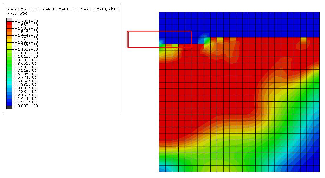
Figure 23 Von mises stress distribution for 0.20m mesh

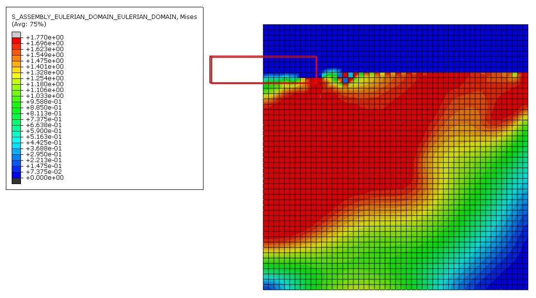
Figure 24 Von mises stress distribution for 0.10m mesh

Figure 25 Von mises stress distribution for 0.05m mesh

Figures 23, 24 and 25 show the von mises stress distribution on the finite element model with a slower loading rate (lower velocity). Screenshots of these stresses were also taken on the last time frame to show the end of the installation stage of the settlement within the time specified. Even in this scenario, the stress is the highest near the corner of the footing for all three cases.

On figure 23, the stress near the corner is +1.732e+00 and occupies almost 4 elements this time, each having a width of 0.20m. On figure 20, the stress near the corner is 1.736e+00 and occupies around 3 elements, each of their width being 0.10m. On figure 21, the stress near the corner is 1.733e+00 and occupies about 3 elements, each of their width being 0.05m. This shows that as the element size gets smaller, the element in the corner of the strip footing is able to distribute the load and put up will the change in displacement better than when it has larger sized elements.

The computer time that is used to run a simulation with a specified mesh by using the explicit time integration is proportional to the time taken for the event. Computational is important when using the mesh size. The following table shows the computational time that was required for each of the analyses. A sample log file from which they were obtained is attached to the appendix.

	Mesh size	Computational time required
Analysis part 1	0.20m	18 sec
	0.10m	46 sec
	0.05m	262 sec
Analysis part 2:   With higher density	0.20m	14s
	0.10m	38s
	0.05m	191s
Analysis part 3:   With lower loading rate	0.20m
	0.10
	0.05

4.2 ERRORS AND LIMITATIONS

One of the biggest limitations faced during this project was that the ABAQUS software had a restriction on the highest number of nodes. Due to this reason, finer meshes could not be generated due to the large number of nodes involved.

CHAPTER 5: CONCLUSION

5.1 SUMMARY

This study summarises the effects of mesh quality on a strip footing with the help of numerical modelling. The finite element model helps replicate and analyse the behaviour o f a real soil when different parameters are applied, along with boundary conditions. Objectives of this paper have been met since the results and simulations obtained from the study can be used to select the optimal mesh size. Keeping in mind both, accuracy of results and the computational time is suitable. After analysing the results in chapter 4, it can be seen that the finest meshes produce the more accurate results than the coarse meshes in all three analysis parts. Therefore, the mesh size of 0.05m was selected to be the most suitable option. The mesh size 0.05m had the least amount of percentage difference (4.44%, 5.03%, 3.86%) when compared among the other two mesh sizes (0.20m and 0.10m) to the analytical value of 5.1416. The 0.20m mesh size had a percentage difference of 12.81, 12.81% and 11.25 %, while the 0.10m mesh had 6.97%, 7.55%, 5.80%. Even though the 0.05m mesh size takes longer computational time, it Is still preferred since the results are much more reliable for the 0.05m mesh size. Some computational time was saved by analysing only half of the model. Furthermore, the results improved further when the loading rate was decreased. The lower velocity of the load lead to more accurate results. Having said all of that, it can be seen that finer mesh quality produces more accurate results than compared to the coarser mesh quality

5.2 RECOMMENDATION FOR FURTHER WORK

Recommendation for further work would be to carry out more number of mesh sizes to have plenty of results to analyse from. Apart from that , the von mises stress – strain curve could’ve have been plotted to see how the curves are affected by the mesh quality.

REFERENCES

Hasan Emre Oktay, B. (2012) ‘FINITE ELEMENT ANALYSIS OF LABORATORY MODEL EXPERIMENTS ON BEHAVIOR OF SHALLOW FOUNDATIONS UNDER GENERAL LOADING’. Available at: http://citeseerx.ist.psu.edu/viewdoc/download?doi=10.1.1.633.4312&rep=rep1&type=pdf (Accessed: 17 March 2017).

‘Introduction to Finite Element Analysis (FEA) or Finite Element Method (FEM)’ (no date). Available at: http://www.engr.uvic.ca/~mech410/lectures/FEA_Theory.pdf (Accessed: 17 March 2017).

Md Nujid, M. and Raihan Taha Professor, M. (no date) ‘A Review of Bearing Capacity of Shallow Foundation on Clay Layered Soils Using Numerical Method’. Available at: http://www.ejge.com/2014/Ppr2014.072mar.pdf (Accessed: 17 March 2017).

‘Module 4 : Design of Shallow Foundations’ (no date). Available at: http://nptel.ac.in/courses/105101083/download/lec17.pdf (Accessed: 3 April 2017).

Potts, D. M. and Zdravković, L. (2001) Finite Element Analysis in Geotechnical Engineering: Volume two – Application. Available at: http://0-www.icevirtuallibrary.com.wam.city.ac.uk/doi/pdf/10.1680/feaigea.27831.0006 (Accessed: 17 March 2017).

Prandtl (1920) ‘Module 4 : Design of Shallow Foundations’. Available at: http://nptel.ac.in/courses/105101083/download/lec17.pdf (Accessed: 5 April 2017).

Skempton (1951) ‘Shallow Foundation I: Ultimate Bearing Capacity’. Available at: http://civilwares.free.fr/Geotechnical engineering – Principles and Practices of Soils Mechanics and Foundation Engineering/Chapter 12.pdf (Accessed: 2 April 2017).

T. More, S. and Bindu, D. R. S. (2008) ‘Effects of mesh size on finite element analysis of plate structure’, Certified International Journal of Engineering Science and Innovative Technology, 9001(3), pp. 2319–5967. Available at: http://www.ijesit.com/Volume 4/Issue 3/IJESIT201503_24.pdf (Accessed: 17 March 2017).

Terzaghi (1943) Terzaghi. Available at: http://www.ce-ref.com/Foundation/Bearing capacity/Terzaghi.html (Accessed: 2 April 2017).

WELCOME TO ENGINEERS CADD CENTRE (P) LTD (no date). Available at: http://www.eccindia.org/eccsite/htmls/whatisfea.html (Accessed: 5 April 2017).

APPENDIX

INPUT FILE FOR 0.05m MESH (similar files were created for 0.10m and 0.20m mesh)

*Heading

*Preprint, echo=NO, model=NO, history=NO, contact=NO

**

*Part, name=Domain

*Surface, type=EULERIAN MATERIAL, name=Eulerian_domain

Eulerian_domain

*End Part

**

*Part, name=Pipe

*End Part

**

**

** ASSEMBLY

**

*Assembly, name=Assembly

*Instance, name=Eulerian_domain, part=Domain

*node

1,0.0,1.0,-0.025

25,1.2,1.0,-0.025

61,3.0,1.0,-0.025

101,5.0,1.0,-0.025

809,0.0,0.6,-0.025

833,1.2,0.6,-0.025

869,3.0,0.6,-0.025

909,5.0,0.6,-0.025

6061,0.0,-2.0,-0.025

6085,1.2,-2.0,-0.025

6121,3.0,-2.0,-0.025

6161,5.0,-2.0,-0.025

10101,0.0,-4.0,-0.025

10125,1.2,-4.0,-0.025

10161,3.0,-4.0,-0.025

10201,5.0,-4.0,-0.025

1000001,0.0,1.0,0.025

1000025,1.2,1.0,0.025

1000061,3.0,1.0,0.025

1000101,5.0,1.0,0.025

1000809,0.0,0.6,0.025

1000833,1.2,0.6,0.025

1000869,3.0,0.6,0.025

1000909,5.0,0.6,0.025

1006061,0.0,-2.0,0.025

1006085,1.2,-2.0,0.025

1006121,3.0,-2.0,0.025

1006161,5.0,-2.0,0.025

1010101,0.0,-4.0,0.025

1010125,1.2,-4.0,0.025

1010161,3.0,-4.0,0.025

1010201,5.0,-4.0,0.025

*nset,nset=base11

1

1000001

*nset,nset=base12

25

1000025

*nset,nset=base13

61

1000061

*nset,nset=base14

101

1000101

*nset,nset=base21

809

1000809

*nset,nset=base22

833

1000833

*nset,nset=base23

869

1000869

*nset,nset=base24

909

1000909

*nset,nset=base31

6061

1006061

*nset,nset=base32

6085

1006085

*nset,nset=base33

6121

1006121

*nset,nset=base34

6161

1006161

*nset,nset=base41

10101

1010101

*nset,nset=base42

10125

1010125

*nset,nset=base43

10161

1010161

*nset,nset=base44

10201

1010201

*nfill,nset=nl1

base11,base12,24, 1

base12,base13,36, 1

base13,base14,40, 1

*nfill,nset=nl2

base21,base22,24, 1

base22,base23,36, 1

base23,base24,40, 1

*nfill,nset=nl3

base31,base32,24, 1

base32,base33,36, 1

base33,base34,40, 1

*nfill,nset=nl4

base41,base42,24, 1

base42,base43,36, 1

base43,base44,40, 1

*nfill,nset=nl10

nl1,nl2,8,101

*nfill,nset=nl20

nl2,nl3,52,101

*nfill,nset=nl30

nl3,nl4,40,101

*nset,nset=bottomtop

nl1

nl4

*Nset, nset= E_nodes

nl10

nl20

nl30

*nset,nset= Left,generate

1,10101,101

1000001,1010101,101

*nset,nset= Right,generate

101,10201,101

1000101,1010201,101

*element, type=EC3D8R

1,103,1000103,1000002,2,102,1000102,1000001,1

*elgen

1,100,1,1,100,101,100

*Elset, elset=E_elements, generate

1,10000,1

*elset,elset=void,generate

1,2000,1

*elset,elset=seabed,generate

2001,10000,1

*Eulerian Section, elset=E_elements

soil, Eulerian_domain

*End Instance

*Instance, name=Pipe-1, part=Pipe

*Node

1, -1.0,  0.0,    0.1

2,  1.0,  0.0,    0.1

3,  1.0,  0.5,    0.1

4, -1.0,  0.5,    0.1

5, -1.0,  0.0,   -0.1

6,  1.0,  0.0,   -0.1

7,  1.0,  0.5,   -0.1

8, -1.0,  0.5,   -0.1

9,  0.0,  0.0,    0.0

*Element, type=R3D4

1,  1,  2,  6,  5

2,  2,  3,  7,  6

3,  3,  4,  8,  7

4,  4,  1,  5,  8

**

*Nset, nset=ref_point

9,

*Elset, elset=pipe_element, generate

1,  4,    1

*End Instance

*Rigid Body, ref node=Pipe-1.ref_point, elset=Pipe-1.pipe_element

*End Assembly

**

*Material, name=soil

*Density

0.1,

*Elastic

400, 0.495

*Mohr Coulomb

0.,0.

*Mohr Coulomb Hardening

1.,0.

*Surface Interaction, name=IntProp-1

*Friction, Taumax=1.0

1.0,

**

** Material assignment

*Initial Conditions, type=VOLUME FRACTION

Eulerian_domain.seabed, Eulerian_domain.Eulerian_domain, 1.

**

*Contact, op=NEW

*Contact Inclusions, ALL EXTERIOR

*Contact Property Assignment

,  , IntProp-1

**——————————————————————–

*Amplitude, name=Amp_g,definition=smooth step

0.,      0.,       1.,     1.

*Amplitude, name=PUSH

0,     0.,    20,    1.

** ——————————————————-Step2_INSTALL

*Step, name=installation

*Dynamic, Explicit

, 2.

*Bulk Viscosity

0.06, 1.2

**

*Boundary, type=VELOCITY

Eulerian_domain.Bottomtop, 1, 3

Eulerian_domain.Left, 1, 1

Eulerian_domain.Right,1,2

Eulerian_domain.E_nodes, 3, 3

Pipe-1.ref_point, 1, 1

Pipe-1.ref_point, 3, 6

Pipe-1.ref_point, 2, 2, -0.05

*Restart, write, number interval=1, time marks=NO

*Output, field,TIME INTERVAL= 0.1, VARIABLES=PRESELECT

*element output,elset=Eulerian_domain.E_elements

EVF,SDV,S

*node output,nset=Pipe-1.ref_point

COORD

*Output, history, TIME INTERVAL= 0.1, VARIABLES=PRESELECT

*node output, nset=Pipe-1.ref_point

RF1, U1,RF2, U2

*End Step

EXCEL WORKSHEET: PROCESSING OF RAW DATA FILES

SAMPLE JOB LOG FILE

Abaqus JOB Job-1

Abaqus 6.14-1

Abaqus License Manager checked out the following licenses:

Abaqus/Explicit checked out 5 tokens from Flexnet server NSQ557AP.enterprise.internal.city.ac.uk.

<395 out of 400 licenses remain available>.

Begin Analysis Input File Processor

07/03/2017 14:19:13

Run pre.exe

07/03/2017 14:19:17

End Analysis Input File Processor

Begin Abaqus/Explicit Packager

07/03/2017 14:19:17

Run package.exe

07/03/2017 14:19:23

End Abaqus/Explicit Packager

Begin Abaqus/Explicit Analysis

07/03/2017 14:19:23

Run explicit.exe

07/03/2017 14:23:34

End Abaqus/Explicit Analysis

Begin Selected Results Translator

07/03/2017 14:23:34

Run select.exe

07/03/2017 14:23:35

End Selected Results Translator

Abaqus JOB Job-1 COMPLETED