Metric Geometry and Metric Space Theory

Info: 9277 words (37 pages) Dissertation
Published: 11th Oct 2021

Reference this

Tagged: Mathematics

Share this: Facebook Twitter Reddit LinkedIn WhatsApp

1.Introduction

2.Metric spaces

The roots of metric spaces

Definition of metric spaces.

Brief history of topology

Definition of topology

Homotopy and homeomorphism

Applications of topology

Raster graphics

Sensor network

4.Coarse geometry

Difference between topology and coarse geometry

Coarse Space

Taxicab metric and application of the metric in a linguistic transport

Embeddings of metric spaces and their applications

5.Summary

6.Bibliography

Introduction

From the time of Euclid (300 B.C.) geometry has been an inseparable part of mathematics. It is concerned with the shape of individual objects, spatial relationships among a variety of objects, and the properties of surrounding space. Geometry is not strictly the study of three-dimensional objects and/or flat surfaces but can even be the abstract thoughts and images which are often described in geometric terms. During Year 2 at the university, I had an amazing opportunity to discover the concept of fractals and write the article about it.

In my dissertation, I would like to explore and investigate in depth a different branch of geometry called metric geometry.

I would like to give a detailed explanation of basic notions and techniques in the theory of metric spaces. This theory experienced a very rapid development in the recent decades and gained access to many other mathematical areas (such as Group Theory, Riemannian Geometry, and Partial Differential Equations). My goal is as well to give a fundamental introduction into a variety of the topics related to the notion of distance in metric geometry.

We think of a metric as a way of measuring a distance between the points in a topological space. The notion of the distance between the points of ideal sets leads to the concept of metric spaces. Further, this concept leads to convergence and Cauchy sequence in the group. The study of Convergence is often reliant on matrices, which are of great importance to such a study. They are often used for the solution of approximation. [50]. Coarse geometry looks at areas only at large scale and neglects little local structures by considering only geometrical properties which are global in nature. Coarse equivalence is same as homomorphism where the features of coarse are invariant.

Within Coarse Geometry the study of discrete metric spaces is of great importance. Subsets being open are often a characterisation of discreteness, however the topological equivalence does not recognize between areas of discreteness beyond the number of elements in a specific set. On the other hand coarse equivalence characterises various discrete spaces [15].

Metric spaces

The roots of metric spaces

There are variety of ways to measure the distance between two points or two vectors. While the generalization of geometry beyond the Euclidean spaces initiated with Italian mathematicians like Ascoli or Volterra, it first received a coherent and abstract research in Fréchet’s doctoral thesis of 1906 where the intuitive notions of Euclidean space beyond the study of geometric figures were adopted [62]. The abstract spaces resulting from such a study were characterized by their particular elements, truism, and their conjunction. In addition, the notion of limits was devised and applied by Fréchet from calculus in treating the functions as elements of a vector space, which was also a way of measuring lengths and distances amid the functions to produce a metric space. He identified two significant kinds of generalized spaces: The L-spaces, where the notion of limit was based on the truism of convergent sequences, and the second being the L-spaces where a distance function can be defined. Research was continued by many other mathematicians e.g. Finsler ,Hausdorf or Wilson and that finally led to the consolidation of the properties of metric spaces.

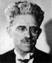
Fig.1 Maurice René Fréchet (Wikipedia,nd.)

To understand what exactly coarse geometry and topology are, there are a number of definitions that I need to explore. I am going to explore open sets, metric spaces, and also closed sets. I am going to move on to the concept of Coarse Geometry and Topology together with their applications. It is worth mentioning that in order to establish the meaning of open and closed sets one would have to really understand the true meaning of Topology.

Definition of metric spaces

A metric space is simply a non-empty set X such that to each x, y ∈ X there corresponds a non-negative number called the distance between x and y. For the function to be considered a metric, there are certain properties of the distance (well known from Euclidean geometry), such as symmetry and the triangle inequality, that need to be satisfied.

Definition 2.1 Let X be a set. A function

d:X×X →Rnis called a metric if it satisfies the following three conditions:

dx,y≥0for all
x,y∈X(Non-negativeness)
dx,y=0 ↔x=y(positive definitness)
dx,y=dx,yfor all
x,y∈X(symmetry)
dx,y≤dx,z+dz,yfor all
x,y, z∈X(triangle inequality)

A pair, where d is a metric on X is called a metric space.

Property 1 expresses that the distance between two points is always larger than or equal to 0. Property 2 states if the distance between x and y equals zero, it is because we are considering the same point. Third property tells us that a metric must measure distances symmetrically. The triangular inequality is a generalization of the famous result that holds for the Euclidean distance in the plane. In order to understand this concept, I need to show a few examples of what does and does not constitute a distance function to that of a metric space..

Example 2.1 The set of real numbers

Rwith the function

d(x, y) = |x – y|is a metric space. More generally, let

Rnn denote the Cartesian product of

Rwith itself n times:

Rn = {(x1, . . . , xn) | xi ∈ R for each i}.

The function

d: Rn × Rn→ R defined by

dx1, . . . , xn,y1, . . . , yn= x1- y12 + · · · + xn – yn2

is a metric on

Rn, called the Euclidean metric. When n = 1, 2, 3, this function gives precisely the usual notion of distance between points in these spaces.

Example 2.2 Suppose f and g are functions in a space

X = {f : [0, 1] → R}. Does

d(f, g) =max|f – g|define a metric?

I need to verify if this function satisfies the criteria of the metric. In this example property number 2 does not hold. It can be proven by considering 2 arbitrary functions at any point within the interval

[0, 1]. If |f(x) – g(x)| = 0, this does not imply that

f = gbecause f and g could intersect at one, and only one, point. Therefore,

d(f, g)is not a metric in the given space.

Open sets

After introducing the notion of distance, I am going to define what it means for the set to be open in a metric space.

Definition 2.2. Let X be a metric space. A ball B of radius r around a point

x ∈ Xis

B = {y ∈ X|d(x, y) < r}.

We can see that this ball encloses all points whose distance is less than r from x.

Definition 2.3. A subset

O ⊆ Xis open if for every point

x ∈ O, there is a ball around x entirely contained in O.

Example 2.3. Let

X = [0, 1].The interval

(0, 12)is open in X.

Example 2.4. Let

X = R. The interval

[0, 12)is not open in X.

If set is open, we should be able to choose any point within the set, take an infinitesimal step in any direction within our given space, and find another point within the open set. In example 3, we can take any point

0 < x < 12 and find a point to the left or right of it, within the space [0, 1], that also is in the open set

[0, 1). However, this approach does not work in Example 4. For instance, if we take the point within the set

[0, 1), say 0, and take an infinitesimal step to the left while staying within our given space X, we are no longer within the set

[0, 1).Therefore, this would not be an open set within

R. Note that if a set is not open, this does not necessary mean that it is closed. Additionally, there are sets that could be neither open, nor closed, and sets that are open and closed.

In conclusion, open sets in spaces X have the following properties:

The empty set is open
The whole space X is open
The union of any collection of open sets is open
The intersection of any finite number of open sets is open.

Closed sets

Before I introduce the concept of a closed set based on the open sets, I would like to define it using the notion of a limit point.

Definition 2.4. A point z is a limit point for a set A if every open set U containing z intersects A in a point other than z.

Note that the point z could or could not be in A. The example I am going to present will make it slightly clearer.

Example 2.5. Consider the open unit disk

D = {(x, y) : x2 + y2 <1}.Any point in D is a limit point of D, for example (0, 0). Any open set U about this point will contain other points in D. What about the point (1,0)? Point

(1, 0),which is not in D. This is still a limit point because any open set about (1, 0) will intersect the disk D.

The theorem and examples below will give us a useful way to define closed sets and will also prove to be very helpful when deciding whether the set is open or not.

Definition 2.5 A set C is a closed set if and only if it contains all of its limit points.

Example 2.6. The unit disk in the previous example is not closed because it does not contain all of its limit points- point (1, 0) to be specific.

Example 2.7. Let

A = Zbe a subset of

R. This is a closed set because it does contain all of its limit points (in this case there is no point which actually is a limit point!). A set that has no limit points is closed, by default, because it contains all of its limit points. Every intersection of closed sets is closed, and every finite union of closed sets is closed.

Topology

The aim of topology

Topology is a relatively young field of mathematics. It deals with topological spaces, this is a collection with a structure describing the neighborhood of the points, which makes it possible to provide a general definition for continuous mappings. Two topological spaces are considered indistinguishable by topological methods if there is a continuous bijection between them, the reverse bijection is also continuous. We are talking then, the spaces are homeomorphic, and the appropriate bijection is called homeomorphism. The main the purpose of the topology is to classify topological spaces, in particular by constructing the so-called invariants, most often certain features, numbers, groups or classes of equivalence to a certain relationship, which are the same for homeomorphic spaces.

It is worth realizing from the very beginning that homeomorphic spaces can be spaces that are everyday they look very different. As a classic example, an example of a completed one is given here torus and a pot with an ear, which are very dissimilar, and yet homeomorphic (Fig.2). Thus, homeomorphism is a relationship that identifies a lot. It can be perceived as a weakness of theory, in fact, it is exactly the opposite: If we do not know much about two spaces, the statement that these spaces are different is often the easiest to achieve by methods topological.

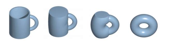
Fig.2 From left: empty mug, filled mag, deformed mug, torus (Wikipedia,n.d.)

The goal of topology is to create tools that allow to distinguish and classify sets (topological spaces), methods that are slightly more demanding than counting the elements of the set (Set Theory), but still allowing the identification of the sets, that seem to be different at the first glance. Topology does not include methods that require measuring angles.

Brief history of topology

Although the topology is a young field, its roots can be found in certain problems analyzed already in the eighteenth and nineteenth centuries.

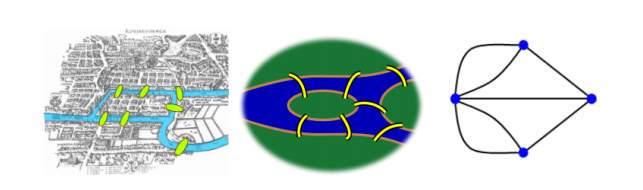
Fig.3 The Seven Bridges of Königsberg problem. From the left: map of Koenigsberg from Euler’s day with Pregel river and bridges; “topological” version of the map abstracting from the shape of the river and the route of streets; graphical representation (Google, n.d.)

The Seven Bridges of Königsberg problem (Fig.3) is about taking a walk through the town, visiting each part of the town and crossing each bridge only once. In 1735, a Swiss mathematician Leonhard Euler showed that this problem has no solution. Method used by Euler is considered the first example of a topological approach to the problem in mathematics.

In 1895, the famous French mathematician Henri Poincaré published the work called Analysis Situs, which is considered the first work in the field of topology. Although the terminology used today is slightly different, in Poincaré’s work we can find the idea of homeomorphic subsets and the method of finding common invariants that describe homeomorphic subsets. In particular, Poincaré introduced combinatorial methods to search for such invariants, which led him to define the so-called Betti numbers for polyhedrons. Figuratively speaking, the kth Betti number refers to the number of k-dimensional holes on a topological surface Poincaré’s publication became a starting point of not only general topology, but also algebraic topology (older name- combinatorial topology).

PSM V82 D416 Henri Poincare.png

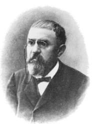
Fig.4 Henri Poincaré [Google, n.d.]

Definition of topology

Topology divides into 2 areas: a general topology and algebraic topology. In algebraic topology we use algebraic tools to compare topological spaces but in general topology these tools are built specifically for the use in area of general topology. Very important topological concepts are: disintegration to pieces and existence of holes. According to Eric Weisstein [64]“A hole in a mathematical object is a topological structure which prevents the object from being continuously shrunk to a point.”

Counting pieces of space, so-called connected components, is related to the study of existence holes in space. Originally, it required narrowing down to the space that can be made “build of blocks” in the form of a tetrahedron or a cube. (Fig.5)

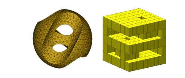
Fig.5 Topological spaces made of tetrahedron blocks (on the left) and cubes (on the right).

Homotopy and homeomorphism

One of the special tools used to study topological spaces is homotopy. Figuratively speaking, homotopy is a continuous deformation of one projection into another.

As mentioned earlier, from a topologist’s point of view doughnut and mug are exactly the same. If they were made out of the rubber, one could be twisted and stretched into the shape of the other object without changing its essence. Very important but quite often confused is the concept of homeomorphism. The characterization of a homeomorphism often leads to confusion with the concept of homotopy, which is actually defined as a continuous deformation, but from one function to another, rather than one space to another. In the case of a homeomorphism, envisioning a continuous deformation is a mental tool for keeping track of which points on space X correspond to which points on Y—one just follows them as X deforms. In the case of homotopy, the continuous deformation from one map to the other is of the essence, and it is not as restrictive, since none of the maps involved need to be one-to-one or onto. Homotopy leads to a relation on spaces: homotopy equivalence.

The formal definition of homeomorphism is as follows.

Definition 3.1 A homeomorphism is a function

f : X → Ybetween two topological spaces X and Y that:

• is a continuous bijection, and

• has a continuous inverse function

f-1.

Different way to describe homeomorphism is presented in Definition 3.2.

Definition 3.2 Two topological spaces X and Y are said to be homeomorphic if there are continuous map

f : X → Y and g : Y → Xsuch that

f ∙ g = IY and g ∙ f = IX

Moreover, the maps f and g are homeomorphisms and are inverses of each other, so we may write

f -1in place of g and

g-1in place of f.

Here, IY and IX denote the identity maps. When inspecting the definition of homeomorphism, it is noted that the map is required to be continuous. This means that points that are “close together” (if a metric is used we would say within the neighborhood) in the first topological space are mapped to points that are also “close together” in the second topological space. Similar observation applies for points that are far apart.

As a final note, the homeomorphism forms an equivalence relation on the class of all topological spaces.

Reflexivity: X is homeomorphic to X.

Symmetry: If X is homeomorphic to Y, then Y is homeomorphic to X.

Transitivity: If X is homeomorphic to Y, and Y is homeomorphic to Z, then X is homeomorphic to Z.

The resulting equivalence classes are called homeomorphism classes.

Applications of topology

Although the topology was created only at the beginning of the 20th century, it quickly gained a status of fundamental area of mathematics. However, it was not until the end of the last century that it was noticed how important are the applications of topology outside of mathematics, including applications in biology, medicine, engineering and information technology. Therefore, since the end of the twentieth century, apart from the theoretical topology, there is also applied and computational topology that experienced a very rapid development in the recent time.

Raster graphics

Raster graphics consist of a large number of squares (pixels) of uniform colors (Fig.6). After performing thresholding (changing darker colors to black, and brighter ones to white) we get a topological space made of blocks (Fig.7), which we can explore with methods used in algebraic topology. The concept of cohesion and a coherent component, one of the basic topological concepts is widely used in the analysis of images. For example, if we want to automate counting the number of craters on the surface of the Moon, we segment the pictures and replace the colors accordingly dark to black and bright to white.

Fig 6 Pixel graphic [Google,n.d.]

Sensor network

Sensor networks are used to monitor areas that require control. It can help with protection of the area against unauthorized people, prevention of fires or contamination. Sensors are normally distributed at random but there is the problem of coverage: whether the whole area is in the range of sensors? The problem can be solved by using topological methods. Sensors communicate with each other through radio network, which allows you to construct a graph of neighborhoods. We can then build a polyhedron in such a way that any coverage gaps appear as holes whose presence may be detected by topological methods.

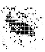
Fig.7 Topological image [Google, n.d.]

Coarse geometry

Difference between topology and coarse geometry

The topology effectively explores metric spaces but focuses on their local properties. Therefore, it becomes completely ineffective when the space is discrete (consists of isolated points)

However, these discrete metric spaces are not always identical (e.g., Z and Z 2). To see differences between them, we should focus on their global “shape” instead of on local properties. In further part of the chapter, I am going to show some examples of discrete metric spaces, for which the inspection of their global structure is very important.

Coarse Space

A coarse structure on a set X is a collection of the subsets of the Cartesian product X × X with certain properties which allows to create the large-scale structure of a metric space.

Definition 4.1Let X and Y be metric spaces and let

f: X → Ybe a map (not necessarily continuous).

The map f is (metrically) proper if the inverse image of each bounded subset of Y is a defined subset of X.
The map f is (uniformly) bornologous if for every
R > 0there is

S > 0such that

d(x,x’) < R ⇒ d(f(x),f(x’)) < S.
The map f is coarse if it is proper and bornologous.

We want our coarse functions to maintain a global “shape” of the space. Therefore, they should not crush (metric property), neither extensively stretch in any direction (bornologous property).

To be able to understand to understand the definitions precisely, it is necessary to determine what functions and spaces are considered to be equal from a coarse point of view.

Definition 4.2. Two maps f, g from X into a metric space Y are close if

d(f(x),f(y))is bounded, uniformly in X [25]. We say that the metric spaces X and Y are coarsely equivalent if there exist coarse maps f: X → Y and g: Y → X such that

f ∙ gand

g ∙ f are close to the identity maps on Y and X, respectively.

Example 4.1 If

X = Y = N, the natural numbers, then the map

n → 12n + 62is coarse, but the map

n → 1is not coarse (it fails to be metrically proper), and the map

n → n2 is not coarse either (it fails to be bornologous).

Also suppose that

R2 and

Rare given their natural metric coarse structures. Then the absolute value map

v → |v|,from

R2to

R, is a coarse map, but the coordinate projections from

R2to

Rare not.

Thanks to the properties listed below it is easy to check the controlled sets associated to a metric space X.

The transpose
Et= {(x, y) : (y, x) ∈ E}of a controlled set

Eis controlled;
The composition
E1 ∙ E2of controlled sets

E1and

E2is controlled:
E1 ∙ E2= {(x, z) ∈ X × X : ∃y ∈ X,(x, y) ∈ E1and(y, z) ∈ E2}
A finite union of controlled sets is controlled;
The diagonal
∆X := {(x, x) : x ∈ X}is controlled:

If our metrics are not allowed to take the value

+∞, then the controlled sets will have one additional property:

The union of all controlled sets is X ×X.

Now I am going to try to axiomatize the situation in a more metric independent way:

Definition 4.3 (coarse structure). Let X be a set. A collection

εof subsets of X × X is called a coarse structure- the elements of

εwill be called controlled-, if the axioms (1-4) hold for E. The pair

(X, ε)is called a coarse space. The coarse space is called unital, if (5) holds and a coarse structure having the property (6) will be called connected.

Definition 4.4 (bounded coarse structure). Let

(X, d)be a metric space, as we saw the metric d induces a coarse structure on X, which is called bounded coarse structure. To make it clear, we can define bounded coarse structure induced by the metric d as follow: Set

Dr := {(x, y) ∈ X × X : d(x, y) < r}. Then

E ⊆ X × Xis controlled, if

E ⊆ Drfor some r > 0.

Definition 4.5 (coarse structure generated by

μ). Let X be a set and

μa collection of subsets of

X×X. Since any intersection of coarse structures on X is itself a coarse structure, we can make the following definition. By

cs(μ)we denote the smallest coarse structure containing

μ, i.e. the intersection of all coarse structures containing

μ. We call cs(

μ) the coarse structure generated by

μ.

Definition 4.6 (close maps). Let

(X, ε)be a coarse space and S a set. The maps

f, g : S → Xare called close if

{(f(s), g(s)) : s ∈ S} ⊆ X × Xis controlled.

Proposition 4.1 Let

(X,ε)be a coarse space, and let D be a subset of X. The following are equivalent:

(1)

D × Dis controlled;

(2)

D × {p}is controlled for some

p ∈ X;

(3) The inclusion map

D → Xis close to a constant map.

Proof.

(1) ⇒ (2)is obvious. For (2) ⇒ (1), since D × {p} is controlled, so {p} × D is also controlled, but

D × D ⊆ (D × {p}) ∙({p} × D) i.e. D × Dis controlled.

(2) ⇔ (3) is also obvious.

Definition 4.7 Let

(X, ε)be a coarse space.

(1)

D ⊆ Xis called bounded if D satisfying one of the above conditions;

(2) a collection

uof subsets of X is called uniformly bounded if

UU∈u U × Uis controlled;

(3) the coarse space X is called separable if it has a countable uniformly bounded cover.

For example, in a bounded coarse structure, the bounded sets are just metrically bounded ones:

D ⊆ Xis bounded if and only if

D × {p}is controlled for some

p ∈ Xand it holds if and only if

D × {p} ⊆ Drfor some

r > 0which means

D ⊆ B(p; r).

Lemma 4.1 In a connected coarse structure, the union of two bounded sets is bounded.

Proof 4.1 Suppose

D1and

D2are two bounded sets in a connected coarse structure X. Since

D1and

D2 are bounded,

D1×{p} and

D2×{q} are controlled for some

p, q ∈ X.But X is connected, so there exists a controlled set E such that

(q, p) ∈ E. Hence

( D2 ×{q})∙Eis controlled and obviously

D2×{p} ⊆ ( D2×{q})∙E, therefore

D2×{p} is controlled. On the other hand

D1 ∪ D2× p= D1 × p∪ D2 × p

So (D1 ∪ BD) × {p}

is controlled, i.e.

D1∪

D2is bounded.

Taxicab metric and application of the metric in a linguistic transport

In transport logistics, the distance that transport means have to play an important role between the place of departure (x) and the destination (y). This problem will affect both one- and two-dimensional space in the case of land and rail transport on land as well three-dimensional spatial transport for air and sea cargo transport. The distance between the place of departure (x) and the destination (y) is strictly dependent on roads and routes as well as the means of transport. The journey from departure cities (x) to the destination (y) cannot always be traveled in the shortest way. Of course, the longer path may be better in another respect, for example, quality. There may be several possible but different routes (roads) of the journey, of which not all will have identical lengths or there may be several routes with equal distances.

We can consider these problems using the theory of metric spaces for strictly defined of metrics tailored to both types of transport means in one, two, three-dimensional spaces as well as those dependent on the available transport routes.

For this purpose, I am going to define Euclidean and non-Euclidean distance metrics in one-dimensional, two-dimensional and three-dimensional spaces.

Euclidean transport distances specify the shortest distance between place of departure (x) and destination (s).

I am going to define the distance metric in transport, as ordered pair (X, ρ), where X is a set of departure places (x,…) and destinations (y,…) where

(x,y)X.

ρ (x, y)is a function with values determining the distance between places x and y. For function ρ to be a function of the metric, it must consist of only real, non-negative. The condition of the transport metric is additionally the fulfillment of the following (mentioned earlier) properties of a metric:

x,y=0  x=y, for x,yX
(x,y)= (y,x), for x,yX
x,y x,z+z,yfor x, y,zX

First property tells that that the distance between two the same locations equals 0. The axiom (2) indicates that for each transport metric the distance from the starting point (x) to the target location (y) is identical to the distance from the destination to the starting place.

The classic Euclidean transport metric determines the shortest distance between two places

i.e. start (x) and target (y). In one-dimensional space 1D of a set of places described by real numbers ℝ Euclid’s metric that satisfies all three properties is given by the following formula:

1 (x, y) =|xy|

and is illustrated graphically in Fig.1.

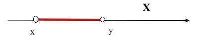
Fig.8 Distance between two places (x) and (y) in one-dimensional Euclid’s space X. (my own work)

In two-dimensional space in the set of places x

x 1, x2and y

(y1, y2)described by real numbers

R2, Euclid metric that satisfies all three properties is given by the following formula:

2(x,y) =[(x1y1)2 +(x2y2)2 ]0.5

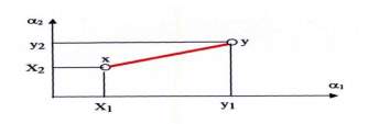
Fig.9 Distance between set of places (x) and (y) in two-dimensional Euclid’s space X. (my own work)

In three-dimensional space in the set of places x

x 1, x2, x3and y

(y1, y2, y3)described by real numbers

R3, Euclid metric that satisfies all three properties is given by the following formula:

3(x,y) =[x1y12 +x2y22+ x3y32 ]0.5

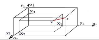
Fig.10 Distance between set of places (x) and (y) in three-dimensional Euclid’s space X. (my own work)

Fig.11 in 2D space, compares the classic, Euclidean metrics with non-Euclidean metrics defining the distances between three places (A), (B), (C) which are at the same time the vertices of the triangle. Fig.11 on the right shows the ADBECFA polygon, which is a triangle in a non-Euclidean transport metric, where the route from A to B leads only through D, route B to C only through E and route C to A through F.

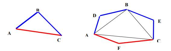
Fig.11 Euclidean space (on the left) and non-Euclidean space (on the right) (my own work)

Fig.12 illustrates the distances described by a non-classical transport metric between towns P, S, Q lying on the solid of the Earth’s ellipsoid and separated by several thousand kilometers from each other. The shortest land route between the P, S, Q places will not be rectilinear, only curvilinear taking into account the curvature of the Earth’s ellipsoid. The shortest route between the towns of P, S, Q described by Euclidean metric could be only achieved by air. Fig.12 illustrates the distances between the vertices of the spherical-elliptical triangle.

Fig.12 An elliptical triangle with PQS vertices lying on the globe with the indicated one non-Euclidean distance metric: b) the triangle on the globe at a closer range, c) The triangle on the plane (my own work)

Taxicab metric

The name of Taxicab metric (or sometimes called Manhattan metric) was given by Americans and it is a form of non-Euclidean metrics of distance. The streets of big cities

and motorways built in the nineteenth century often had a form of regularly intersecting lines at right angles with rectangular surfaces impassable area of buildings and agricultural land. Therefore, it was impossible to reach the destination using the shortest route. In two-dimensional space, a taxicab metric that meets the properties of the metric and consists of the set of numbers described by real numbers ℝ is defined by the following formula:

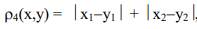
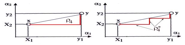
Fig.13 Distance between two places in taxicab metric in two-dimensional space. (my own work)

In three-dimensional space, we can describe the taxicab metric as follows:

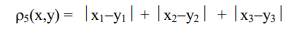
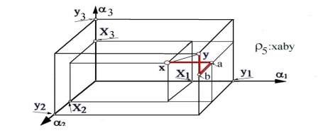
Fig.13 Distance between two places in taxicab metric in three-dimensional space. (my own work)

The method of Taxicab metric is applied in many factories to help with finding the routes for intelligent, self-propelled transport trolleys to move loads horizontally and vertically in large production halls, e.g. in the Federal Mogul in Wiesbaden as well as in the largest European prosthetic factory Otto Bock in Dudenstadt, Germany.

Embeddings of metric spaces and their applications

Given the advances in the recent innovation that allows to secure massive amounts of data, and the consequent, rapid growth of large and complex datasets in a variety of applied fields, computational approaches for signaling/identifying meaningful patterns in such inputs are in enormous demand. The study of quantitative and computational aspects of metric spaces and their embeddings is presented prominently in the study of problems arising when it comes to analysing such massive data provided with a geometric representation. These problems include similarity search, visualization, clustering, and data compression. Analytic and computational methods in Metric Geometry provide crucial insights into the solution of these problems. The theory of Metric Embeddings provides a connection between mathematics, and computer science, leading to powerful new algorithmic methods in the mentioned circumstances.

The theory of embeddings of finite metric spaces has attracted much attention in recent decades by several communities: mathematicians, researchers in theoretical Computer Science as well as researchers in the networking community and other applied fields of Computer Science.

One of the objectives of the field is to find embeddings of metric spaces into other more simple and structured spaces that have low distortion. Given two metric spaces

(X, dX)and

(Y, dY )an injective mapping

f : X → Yis called an embedding of X into Y.

An embedding is non-contractive if for every

u ≠ v ∈ X: dY (f(u), f(v)) ≥ dX(u, v).The distortion of a non-contractive embedding f is:

dist(f) = supU≠VϵX distf (u, v), where

distf (u, v) = dY (f(u),f(v))dX(u,v). Equivalently, the distortion of a non-contracting embedding is the infimum over values α such that f is α-Lipschitz.

We say that X embeds in Y with distortion α if there exists an embedding of X into Y with distortion α. In Computer Science, these embeddings have played a vital role, in recent times, in the evolution of algorithms. More general practical use of embeddings can be found in a vast range of application areas including computer vision, computational biology, machine learning, networking and statistics, among others. From a mathematical perspective embeddings of finite metric spaces into normed spaces are regarded as natural non-linear analogues to the local theory of Banach spaces, which deals with finite dimensional Banach spaces and convex bodies. The most classic fundamental question is that of embedding metric spaces into Hilbert Space.

Major effort has been put into investigating embeddings into

LPnormed spaces.

The foundation of the field has been laid by Bourgain’s following theorem:

Theorem 1 For every n-point metric space there exists an embedding into Euclidean space with distortion

O(log n).

Above theorem is the starting point for theory of embedding into finite metric spaces. Bourgain’s embedding presents an embedding in

Lp, for any

1 ≤ p ≤ ∞with distortion

O(log n)and the dimension of the

Lpspace may be at most

O(log2 n).This result can be extended in the following way: by presenting an embedding with average distortion

O(1)and dimension

O(log n), while maintaining

O(log n)distortion. The results on the average distortion and

lq-distortion can also be extended to infinite compact metric spaces. The intrinsic dimension of a metric space, which may be defined as its doubling dimension, is one of the best possible dimension one can hope for (embedding into less dimensions may show arbitrarily high distortion).

Assouad [61] presents that for a metric space

(X, d)a” snowflake” version of the metric,

(X, dγ )for any

0 < γ < 1can be embedded into Euclidean space with constant distortion and dimension, where the constant depends only on the doubling dimension of the metric and on

γ. He conjectured that the same holds for

(X, d), i.e. the case

γ = 1. A natural variation on Assouad’s conjecture, is whether a constant dimension can be obtained with low distortion.

Embedding finite metric spaces into tree metrics has been a successful and fertile line of research. These embeddings present quite a simple structure, that can be exploited to show efficient approximation algorithms to a variety of problems. The main points of work focused on probabilistic embedding into trees, and graphs into spanning trees of the graph are

• An embedding with

O(log n) expected distortion into dominating ultrametrics (special type of tree defined in the sequel), which can also be stated as an embedding into a single dominating tree with

O(log n) average distortion.

• An Embedding of a graph into a distribution of spanning trees of the graph with

O(log2 n log log n) distortion.

Summary

Few years ago, I would not expect to make myself familiar with such topic due to its complexity and depth. Today I am extremely happy that I had an opportunity to explore this truly amazing area of mathematics. Through my perseverance I have manages to overcome some hurdles.

To sum up, I would like mention about the key points of my dissertation. As we already know Large-scale geometry is the study of geometric objects viewed from afar. In this type of geometry two objects are considered to be the same, if they look roughly the same from a large distance. For example, when viewed from a greater distance the Earth looks like a point, while the real line is not much different from the space of integers. In the past decades, mathematicians have discovered many interesting and beautiful properties of space metric, which have important applications in both topology and coarse geometry.

A major focus in coarse geometry is the study of discrete metric spaces. Since discreteness is characterized by all subsets being open, topological equivalence does not differentiate between discrete spaces beyond their cardinality. Coarse equivalence, on the other hand, provides a way of categorizing various discrete spaces. Coarse spaces are sets equipped with a coarse structure, which describes the behaviour of the space at a distance. One can obtain some intuition on the concept by considering an extremely zoomed-out view of a space, under which for example the spaces Z and R look similar.

After initial definitions, a method of deriving a coarse structure from a metric is obtained. This is similar to how a metric induces a topology or some other topological structure, but the properties described are majorly the opposite of those described by topology. The closest topological counterpart to coarse structures is the concept of uniform structures. I have also discussed a variety of applications in coarse geometry and topology.

Bibliography

1. J.W. Bandler, R.M. Biernacki, S.H. Chen, P.A. Grobelny, and R.H. Hemmers, “Space mapping technique for electromagnetic optimization,” IEEE Trans. Microwave Theory Tech., vol. 42, no. 12, pp. 2536-2544, Dec. 1994.

2. J.W. Bandler, R.M. Biernacki, S.H. Chen, R.H. Hemmers, and K. Madsen, “Electromagnetic optimization exploiting aggressive space mapping,” IEEE Trans. Microwave Theory Tech., vol. 43, no. 12, pp. 2874-2882, Dec. 1995.

3. A.J. Booker, J.E. Dennis, Jr., P.D. Frank, D.B. Serafini, V. Torczon, and M.W. Trosset,”A rigorous framework for optimization of expensive functions by surrogates,” Structural Optimization, vol. 17, no. 1, pp. 1-13, Feb. 1999.

4. J.W. Bandler, Q. Cheng, S.A. Dakroury, A.S. Mohamed, M.H. Bakr, K. Madsen and J. Søndergaard, “Space mapping: the state of the art,” IEEE Trans. Microwave Theory Tech., vol. 52, no. 1, pp. 337-361, Jan. 2004.

5. T.D. Robinson, M.S. Eldred, K.E. Willcox, and R. Haimes, “Surrogate-Based Optimization Using Multifidelity Models with Variable Parameterization and Corrected Space Mapping,” AIAA Journal, vol. 46, no. 11, November 2008.

6. M. Redhe and L. Nilsson, “Optimization of the new Saab 9-3 exposed to impact load using a space mapping technique,” Structural and Multidisciplinary Optimization, vol. 27, no. 5, pp. 411-420, July 2004.

7. J.E. Rayas-Sanchez, “Power in simplicity with ASM: tracing the aggressive space mapping algorithm over two decades of development and engineering applications”, IEEE Microwave Magazine, vol. 17, no. 4, pp. 64-76, April 2016.

8. J.W. Bandler and S. Koziel “Advances in electromagnetics-based design optimization”, IEEE MTT-S Int. Microwave Symp. Digest (San Francisco, CA, 2016).

9.Franz, Wolfgang (1967), General Topology, Harrap

10. Hocking, John G. & Gail S. Young (1988), Topology, Dover Publications, ISBN 0-486-656764

11. J.L. Kelley (1955), General topology, van Nostrand

12. Steen, Lynn Arthur & J. Arthur Jr. Seebach (1978), Counterexamples in Topology, Berlin, New York: Springer-Verlag, ISBN 0-387-90312-7

13. Bingtuan Hsiung, On the Equivalence and Non-Equivalence of James Buchanan and Ronald Coase

14. R. H. Coase, The Coase Theorem and the Empty Core: A Comment

15. W., F. P. Principles of Geometry (2) Higher Geometry: An Introduction to Advanced Methods in Analytic Geometry (3) Elements of Projective Geometry

16. Stahl, Saul, Stenson, Introduction to Topology and Geometry (Stahl/Introduction) || Informal Topology

17. Basic Concepts in Geometry—An Introduction to Proof (Tt)by Frank B. Allen; Betty Stine Guyer

18. Hüseyi̇n Çakallı, Ayşe Sönmez, Çi̇ğdem Genç, On an equivalence of topological vector space valued cone metric spaces and metric spaces

19. Kumam, Poom, Dung, Nguyen Van, Hang, Vo Thi Le Some Equivalences between Cone -Metric Spaces and -Metric Spaces

20. Kyriakos Keremedis, Eleftherios Tachtsis, On Lindelöf Metric Spaces and Weak Forms of the Axiom of Choice

21. Jinxiu Li, Qin Wang, Remarks on coarse embeddings of metric spaces into uniformly convex Banach spaces

22. Kelly, L. M. [Lecture Notes in Mathematics] The Geometry of Metric and Linear Spaces Volume 490 || On some aspects of fixed point theory in Banach spaces

23. Mihai Turinici, Mean Value Theorems on Abstract Metric Spaces

24. Zhou, C., Chen, D., Zhang, X.B., Chen, Z., Zhong, S.Y., Wu, Y., Ji, G., Wang, H.W. , The roles of geometry and topology structures of graphite fillers on thermal conductivity of the graphite/aluminum composites

25. Emily Reihl, Category Theory in Context

26. N. Higson, J. Roe and G. Yu, A coarse Mayer-Vietoris sequence, Mathematical Proceedings of the Cambridge Philosophical Society, (1993).

N. Higson and J. Roe, The Baum-Connes conjecture in coarse geometry, In Novikov Conjectures, Index Theorems and Rigidity, LMS Lecture Notes, Cambridge University Press, (1995), 227.

28. J. Roe, Lectures on coarse geometry, American Mathematical Society, University Lecture serise, 31(2003).

J. Roe, What is a coarse space? Notices of the American Mathematical Society, 53(6) (2006), 668-669.

M. DeLyser, B. LaBuz, and B. Wetsell, A coarse invariant for all metric spaces, Mathematics Exchange 8 (2011), no. 1, 7–13.

31. Takuma Imamura, Nonstandard methods in large scale topology, in preparation, arXiv:1711.01609.

32. A. Fox, B. LaBuz, and R. Laskowsky, A coarse invariant, Mathematics Exchange 8 (2011), no. 1, 1–6.

33. Brittany Miller, Laura Stibich, and Julie Moore, An invariant of metric spaces under bornologous equivalences, Mathematics Exchange 7 (2010), no. 1, 12–19.

34. Brittany Miller, Laura Stibich, and Julie Moore, An invariant of metric spaces under bornologous equivalences, Mathematics Exchange 7 (2010), no. 1, 12–19.

35. M. E. B. Bekka, P.-A. Cherix, and A. Valette. Proper affine isometric actions of amenable groups. In Novikov conjectures, index theorems and rigidity, Vol. 2 (Oberwolfach, 1993), volume 227 of London Math. Soc. Lecture Note Ser., pages 1–4. Cambridge Univ. Press, Cambridge, 1995.

36. Greg Bell and A. Dranishnikov. Asymptotic dimension. Topology Appl., 155(12):1265–1296, 2008.

37. N. Brodskiy and J. Dydak. Coarse dimensions and partitions of unity. Rev. R. Acad. Cienc. Exactas F´ıs. Nat. Ser. A Mat. RACSAM, 102(1):1–19, 2008.

38. Sergei Buyalo and Viktor Schroeder. Elements of asymptotic geometry. EMS Monographs in Mathematics. European Mathematical Society (EMS), Zu¨rich, 2007.

39. J. Dydak and C. S. Hoffland. An alternative definition of coarse structures. Topology Appl., 155(9):1013–1021, 2008.

40. Cencelj, J. Dydak, and A. Vavpetic. Property A and asymptotic dimension. arXiv:0812.2619, 2008.

41. Piotr W. Nowak. Coarsely embeddable metric spaces without Property A. J. Funct. Anal., 252(1):126–136, 2007

42. Piotr Nowak and Guoliang Yu. What is … Property A? Notices Amer. Math.

43. Pierre de la Harpe. Topics in geometric group theory. Chicago Lectures in Mathematics. University of Chicago Press, Chicago, IL, 2000.

44. A. N. Dranishnikov. Groups with a polynomial dimension growth. Geom. Dedicata, 119:1–15, 2006.

45. Bernd Grave. Asymptotic dimension of coarse spaces. New York J. Math., 12:249– 256 (electronic), 2006.

46. Nigel Higson and John Roe. Amenable group actions and the Novikov conjecture. J. Reine Angew. Math., 519:143–153, 2000.

47. Thomas Jech. Set theory. Springer Monographs in Mathematics. Springer-Verlag, Berlin, 2003. The third millennium edition, revised and expanded.

48. Tom Leinster, Basic category theory

49. Lectures on Coarse Geometry by John Roe.

50. Karlhede, A., 1980. A review of the geometrical equivalence of metrics in general relativity. General Relativity and Gravitation. 12(9). pp.693-707.

51. Chávez, E., Baeza-Yates, R. and Marroquín, J.L., 2001. Searching in metric spaces. ACM computing surveys (CSUR). 33(3). pp.273-321.

52. Anderson, J.E. and Putnam, I.F., 1998. Topological invariants for substitution tilings and their associated $ C^ast $-algebras. Ergodic Theory and Dynamical Systems. 18(3). pp.509-537.

53. Alber, Y.I., 1996. Metric and generalized projection operators in Banach spaces: properties and applications. Lecture Notes in Pure and Applied Mathematics. 19(8). pp.15-50.

54. Niblo, G.A. and Reeves, L.D., 1998. The geometry of cube complexes and the complexity of their fundamental groups. Topology. 37(3). pp.621-633.

55. Kendall, D.G., 1984. Shape manifolds, procrustean metrics, and complex projective spaces. Bulletin of the London Mathematical Society. 16(2). pp.81-121.

56. Havas, P., 1964. Four-dimensional formulations of Newtonian mechanics and their relation to the special and the general theory of relativity. Reviews of Modern Physics. 36(4). p.938.

57. Norton, J., 1985. What was Einstein’s principle of equivalence?. Studies in history and philosophy of science Part A. 16(3). pp.203-246.

58. Lawvere, F.W., 2003. Metric spaces, generalized logic, and closed categories. Rendiconti del seminario matématico e fisico di Milano. 43(1). pp.135-166.

59. Feldman, J., 2005. Equivalence and perpendicularity of Gaussian processes. Pacific Journal of Mathematics. 8(4). pp.699-708.

60. Zabrejko, P.P., 2007. K-metric and K-normed linear spaces: survey. Collectanea Mathematica. 48(4). pp.825-859.

61.Assouad, P. (1983). Plongements lipschitziens dans R. France: Bull. Soc. Math, pp.429–448.

62.Taskovic´, M. (2015). Frechet’s metric spaces–100th next. Mathematica Moravica, 9, pp.69–75.

63.Babinec, T. and Best, C. (2007). Introduction to Topology. [ebook] Available at: http://www.math.colostate.edu/~renzo/teaching/Topology10/Notes.pdf.

64. Weissten, E. (n.d.). Hole — from Wolfram MathWorld. [online] Mathworld.wolfram.com. Available at: http://mathworld.wolfram.com/Hole.html.

RECORD OF PROJECT SUPPORT RECEIVED

Student: Ewa Karpowicz Superviser: Charlie Morris

TIME LINE	Date of support	Nature of support / Summary of Discussion / Suggestions for a way forward	Action by Tutor	Action by trainee	Time used
1	06/02/18	Sending the outline of the dissertation
2	17/05/18	Looking at the full draft of the dissertation. Help with referencing. Advice to extend on the definition of the concept of metric spaces. Advice to motivate each chapter.			30min