Aerodynamic Numerical Analysis of Blunt Body Using CFD

Chapter 1

INTRODUCTION

This section describes the introduction of the project “Aerodynamic Numerical Analysis of Blunt Body Using CFD”. It also explains the preface existing problems of aerodynamic heating, relation between aerodynamic heating and bluntness, why blunt bodies, present case study and conclusion of blunt bodies. Hence, describing the overall view of the problem and its description.

1.1 Preface

“Numerical investigations of drag reduction for a 120⁰ blunt cone at hypersonic flow conditions”

Wave drag is an important parameter to be considered in designing high speed vehicles. It is well known that drag can be alleviated by modifying the flow field in front of the body. There are several techniques to the flow field ahead of a supersonic/hypersonic body and the use of retractable nose spike appears to be simplest and at an efficient means of reducing drag on the vehicle by bringing about flow separation and altering the shock structure around the body.  The present work involves study of hypersonic flow around the blunt nose of an aero vehicle. Three different types of spike have been considered for the purpose of drag reduction studies. These computational studies suggest that flat aero disc is superior to the other two. The numerical results have been validated with experimental data.

Mesh generation as explained in [1] and [20] is a critical starting point for CFD. Currently the generation of high quality hexahedral/quadrilateral meshes for complicated geometries requires tremendous amount of tedious human interaction.  In a CFD project, over 50% of time is spent in mesh generation itself.  The effort required in generating the mesh depends on the complexity of the geometry and physics of the problem.  This necessitates the user to have a good knowledge of geometry and physics of the problem. Grid refinement is the main tool at the disposal of the CFD user for the improvement of the accuracy of the simulation and also to obtain grid independent solution [1, 2].

The user would typically perform a simulation coarse mesh first to get an impression of overall features of a solution. Subsequently the grid is refined in stages until no (significant) differences on the results occur between successive grid refinement stages. Results are then called “grid independent”.  It is usual practice to obtain four qualities of grid which are relatively coarse, medium, fine and super fine.  The superfine grid was adopted for simulating the flow over all the geometries of blunt cone (without spike and with spike). Although many codes/computational methods have been developed to solve the flow fields around the complex body shapes flying at hypersonic mach numbers, the validation of these codes against the standard available/experimental results play a vital role in application engineering. Using CFD, the realistic flow problems can be solved virtually with the help of digital computers. These problems are from different areas such as aerodynamics, automotives, thermal power plants, nuclear power plants etc.

The continual rapid growth of commercial CFD packages and computer power has made the technology accessible to almost all levels of engineering. Despite this rapid growth in the ease of use, speed and robustness of the tool, considerable expertise is still required to ensure the accurate simulations are achieved.  Hence, it becomes necessary to validate the code prior to its use for solving the practical problems. This can be done by solving a problem for which the standard results are available.

1.2 Aerodynamic Heating Problem

If an object cruise at very high suborbital speed (Hypersonic), the shock wave attached to it is very strong. And consequently the temperature behind the shock will be extraordinarily high. And this heat inputs directly to the body.

For example, during the suborbital speed 11.2 km/s the air temperature behind the shock wave reaches the 11,000˚K higher than the surface of the sun. At these high temperatures, the air itself breaks down and the O2 and N2 molecules dissociate into O and N atoms and ions respectively.

The air becomes chemically reacting gas and the heat inputs directly to the vehicle itself. As shown in the Figure 1.1, the vehicle is sheathed in a layer of hot air, first from the hot shock layer at the nose, then from the hot boundary layer on the forward and rearward surface. These hot gases then flow downstream in the wake of the vehicle. So the major objective of entry vehicle design is to shield the vehicle from the severe aerodynamic heating.

The objective of full re-entry vehicle design is to minimize the heat which goes into the vehicle and maximize that which go into the air. So properly designed re-entry vehicle will work as heat shield and reduces the aerodynamic drag.

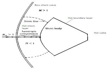
Figure 1.1: Front Shape of a Blunt Body

1.3 Relation Between Aerodynamic Heating and Bluntness

Aerodynamic heating is quietly related to the bluntness of the object. There is a dimensionless factor which relates the heat transfer rate and the free stream velocity known as Stanton number and is defined as,

CH  =dQdTρ∞V∞(h0-hw)S

1.1

Where

ρ∞and

V∞are the free stream density and velocity respectively,

hois the total enthalpy (defined as the enthalpy of a fluid particle that is slowed adiabatically to zero velocity.),

hwis the enthalpy at the aerodynamic surface. Sis the reference area (cross-sectional area of a body).

dQdTIs the heat transfer rate (energy per second) going into the surface from the equation 1.1, a precise result can be expected that relates the heat input to the body to the basis shape of the body.

dQdT=ρ∞V∞ho-hw                                             1.2

Now considering the energy equation that relate the enthalpy energy to the free stream velocity,

ho=hw+V∞2                                    1.3

For a high speed entry vehicle the velocity will very high and the flow ahead of the body will cool enough. From the definition of total enthalpy energy,

ho=Cp

T                                                                    1.4

Temperature associated with the

holarge as compared to the temperature associated with

hwso we can easily make an assumption that,

ho≫hw

1.5

And

hw≈01.6

Applying this assumption to the equation 1.2 gives,

dQdT=12ρ∞V∞SCH

1.7

From the equation 1.7, it can be said that the aerodynamic heating rate varies with the cube of velocity. While studies show that the aerodynamic drag varies as the square of the velocity. So the aerodynamic heating is the sever problem in high speed flight. For this reason, at very high velocities aerodynamic heating becomes a dominant aspect and drag retreat into the background.

The total heat Q is the total amount of energy transferred to the body from beginning to the end of re-entry. The result for Qwill give some vital information on the desired shape for entry vehicles. So, first aerodynamic heating and skin friction will be related with the help of Reynolds analogy. It gives a sense that aerodynamic heating and skin friction should somehow be linked because both are influenced by the friction in the boundary layer. So from Reynolds analogy based on experiments and theory, Stanton number and coefficient of friction can be related as,

CH≈12CF

1.8

Where

CFis the mean skin friction coefficient averaged over the complete surface

On substituting equation 1.8 into equation 1.7 gives,

dQdT=12ρ∞V3∞SCH

1.9

The general equation of motion for atmospheric entry is,

-D

sin⁡θ+W m dV/dT                                               1.10

Where the Dis drag and W is weight of the re-entry body. But the drag is much larger than the vehicle weight, so

D>>W                                                                  1.11

From the equation1.10

dV∞dt=-Dm-12mSCdρ∞V2∞

1.12

And

dQdT=dQdV∞dV∞dt=dQdV∞(-12mSCdρ∞V2∞

)                       1.13

Equating Equation 1.13 and Equation 1.9

dQdV∞(-12mSCdρ∞V∞

)

=14ρ∞V3∞CFS                           1.14

After simplifying equation 1.14 and integrating for Q it will give the total aerodynamic heating as

Qtotal=CFCD12

(

12mV2)                                           1.15

1.4 Types of Blunt Bodies

There are two different aerodynamic configurations, first one is a slender body and other is a blunt body which has a high form drag as shown in Figure 1.2.

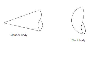
Figure 1.2: Aerodynamic Slender and A Blunt Body

1.4.1 A Sharp Nosed Slender Body Such As a Cone

From the aerodynamics point of view, for a slender body, the skin friction drag is large as compared to the pressure drag hence

Cd≈Cf

Or

CdCf≈1            1.16

So from the equation 1.1 this configuration increase the aerodynamic heating

1.4.2 A Blunt Body Such As a Semi Sphere

For a blunt body, the pressure drag is large in comparison to the skin friction drag hence

Cd ≈Cdp

Or

CfCd≪1         1.17

If

CfCdwill be less, than the total aerodynamic heating will also be less from equation 1.15. So to minimize the re-entry heating, the vehicle must have a blunt nose. That’s why blunt bodies are used for the hypersonic vehicles in practice.

1.4.3 Conclusions of Blunt Body

1. To minimize entry heating, the vehicle must have a blunt nose.
2. The advantages of a blunt body can also be reasoned on a purely physical basis.
3. The computational investigation of minimum-drag bodies at supersonic and moderate hypersonic speeds (Mach 3-12) confirms that, the bodies with the lowest wave drag have to be geometrically blunt.

1.5 Flow Field Around the Blunt Bodies

Due to bluntness of the body, the deflection angle of the body will be large and the strong bow shock will generate in the front of the body. This shock will produce a large gradient of flow property across itself. At the apex of the body the substantial portion of the wave can be assumed as normal 16 shocks, and this portion of the wave will be strongest. Due to this normal shock, temperature of extensive region of the air will be high, and much of this high temperature air will simply flow past the body without encountering the surface.

A blunt body will deposit much of its initial kinetic energy and potential energies into heating the air, and little into heating the body. In this fashion, a blunt body tends to minimize the total heat input to the vehicle. After flow passing through nose, a thin hot boundary layer will generate adjacent to the surface and the flow will separate further and a hot wake region will be formed.

1.6 Shock Wave Interaction in Blunt Bodies in Hypersonic Flow

A blunt body in a high Mach number flow stands with the detached shock waves. These shock waves can be treated as

1. Normal shock wave
2. Oblique shock wave

1.6.1 Normal Shock Wave

The shocks waves that are situated at right angle to the flow are called normal shock waves. These waves are thin regions (approximately .000005m), where the flow property changes drastically. The velocities before and after the shock are at right angles to the shock wave. Substantial portion of the bow shock at the apex can be treated as normal shock. Studies show that the flow after the normal shock will always be subsonic.

1.6.2 Oblique Shock Wave

If the shock wave is located at some angle to the upstream flow, it is called an oblique shock. In the oblique shock wave flow turns into itself. And the strength of the shock depends on the deflection angle and the Mach number. As the Mach number increase, the oblique shock becomes strong. And as the deflection angle increase, the shock becomes strong and after a certain deflection angle of the body, it gets detached from the body. When the maximum deflection angle is exceeded, a detached shock is commonly seen on blunt bodies, but may also be seen on sharp bodies at low Mach numbers.

1.6.3 Shock Wave Formation

Violent disturbances such as results from detonation of explosives, from the flow through rocket nozzles, from supersonic flight of projectiles or from impact on solids differ greatly from the linear phenomena of sound, light or electromagnetic signals. In contrast to the later, their propagation is governed by non-linear differential equations and as a consequence the familiar laws of superposition, reflection and refraction are to be valid; but even more novel features appear, among which the occurrence of shock fronts is the most conspicuous. Across the shock fronts the medium undergoes sudden and often considerable changes in velocity, temperature and pressure. Even when the start of the motion is perfectly continuous, shock discontinuities may later arise automatically. Understanding and control of shock wave phenomena [12] is a matter of obvious importance.

In the supersonic flows of inviscid fluid flows modelled by Euler equations, shock waves appear when the flows are obstructed by solid bodies. Consider the flow of a fluid over a blunt body, as shown in the Figure 1.3. The fluid flow consists of moving and colliding molecules. Some of the molecules collide with the solid body and get reflected. Thus, there is a change in the momentum and energy of the molecules due to their collision with the solid body.

The random motion of the molecules communicates this change in momentum and energy to other regions of the flow. At the macroscopic level, this can be explained as the propagation of pressure pulses. Thus, the information about the presence of the body will be propagated throughout the fluid, including directly upstream of the flow, by sound waves. When the incoming fluid flow has velocities which are smaller than the speed of the sound (i.e., the flow is subsonic), then the sound waves can travel upstream and the information about the presence of the solid body will propagate upstream. This leads to the turning of the streamlines much ahead of the body, as shown in the Figure 1.3.

Now, consider the situation in which the fluid velocities are larger than the speed of the sound (i.e., the flow is supersonic). The information propagation by sound waves is now not possible upstream of the flow. Therefore, the sound waves tend to coalescence at a short distance ahead of the body. This coalescence forms a thin wave, known as the shock wave, as shown in the Figure 1.3.

The information about the presence of the solid body will not be available ahead of the shock wave and, therefore, the streamlines do not change their direction till they reach the shock wave. Behind the shock wave, the flow becomes subsonic and the streamlines change their directions to suit the contours of the solid body. Thus, the shock waves are formed when the supersonic flow is obstructed by a solid body.

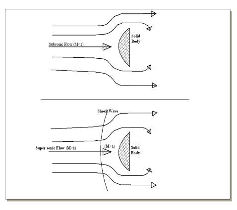
Figure 1.3: Subsonic And Supersonic Flow Over A Solid Body With The Shock Formation

1.7 Drag

In fluid dynamics, drag (sometimes called air resistance or fluid resistance) refers to forces that oppose the relative motion of an object through a fluid (a liquid or gas). Drag forces act in a direction opposite to the oncoming flow velocity. Unlike other resistive forces such as dry friction, which is nearly independent of velocity, drag forces depend on velocity. For a solid object moving through a fluid, the drag is the component of the net aerodynamic or hydrodynamic force acting opposite to the direction of the movement.

The component perpendicular to this direction is considered lift. Therefore drag opposes the motion of the object, and in a powered vehicle it is overcome by thrust. In aerodynamics and depending on the situation, atmospheric drag can be regarded as an inefficiency requiring expense of additional energy during launch of the space object or as a bonus simplifying return from orbit.

1.7.1 Drag coefficient

In fluid dynamics, the drag coefficient (C_d) is a dimensionless quantity that is used to quantify the drag or resistance of an object in a fluid environment such as air or water. It is used in the drag equation, where a lower drag coefficient indicates the object will have less aerodynamic or hydrodynamic drag. The drag coefficient is always associated with a particular surface area.

The drag coefficient of any object comprises the effects of the two basic contributors to fluid dynamic drag, skin friction and form drag. The drag coefficient of a lifting airfoil or hydrofoil also includes the effects of lift induced drag. The drag coefficient of a complete structure such as an aircraft also includes the effects of interference drag. The drag coefficient C_d is defined as:

Cd=Fd12ρv2A                  1.18

Where, F_d is the drag force, which is by definition the force component in the direction of the flow velocity, ρ is the mass density of the fluid, v is the speed of the object relative to the fluid, and A is the area. The reference area depends on what type of drag coefficient is being measured. For aerofoil and many other objects.

1.8 Drag on Object

An object moving through a gas or liquid experiences a force in direction opposite to its motion. Terminal velocity is achieved when the drag force is equal in magnitude but opposite in direction to the force propelling the object. In fluid dynamics, drag (sometimes called resistance) is the force that resists the movement of a solid object through a fluid (a liquid or gas).

Drag is made up of friction forces, which act parallel to the object’s surface plus pressure forces, which act in a direction perpendicular to the object’s surface. For a solid object moving through a fluid, the drag is the sum of all the aerodynamic or hydrodynamic forces in the direction of the movement. Forces perpendicular to this direction are considered lift. It therefore acts to oppose the motion of the object, and in a powered vehicle it is overcome by thrust.

Figure 1.4: Drag On Object

Types of drag are generally divided into three categories

Parasitic drag: Parasitic drag includes form drag, skin friction, and interference drag.

Lift-induced drag: Lift-induced drag is only relevant when wings or a lifting body are present, and is therefore usually discussed either in the aviation perspective of drag, or in the design of either semi-planning or planning hulls

Wave drag: Wave drag occurs when a solid object is moving through a fluid at or near the speed of sound in that fluid.

The overall drag of an object is characterized by a dimensionless number called the drag coefficient, and is calculated using the drag equation. Assuming a constant drag coefficient, drag will vary as the square of velocity. Thus, the resultant power needed to overcome this drag will vary as the cube of velocity. The standard equation for drag is one half the coefficient of drag multiplied by the fluid density, the cross sectional area of the specified item, and the square of the velocity. Drag is the aerodynamic force that opposes an aircraft’s motion through the air. Drag is generated by every part of the airplane (even the engine).

Drag is a mechanical force. It is generated by the interaction and contact of a solid body with a fluid (liquid or gas). It is not generated by a force field, in the sense of a gravitational field or an electromagnetic field, where one object can affect another object without being in physical contact. For drag to be generated, the solid body must be in contact with the fluid. If there is no fluid, there is no drag. Drag is generated by the difference in velocity between the solid object and the fluid. There must be motion between the object and the fluid. If there is no motion, there is no drag. It makes no difference whether the object moves through a static fluid or whether the fluid moves past a static solid object.

Drag is a force and is therefore a vector quantity having both a magnitude and a direction. Drag acts in a direction that is opposite to the motion of the aircraft. Lift acts perpendicular to the motion. There are many factors that affect the magnitude of the drag. Many of the factors also affect lift but there are some factors that are unique to aircraft drag. We can think of drag as aerodynamic friction, and one of the sources of drag is the skin friction between the molecules of the air and the solid surface of the aircraft. Because the skin friction is an interaction between a solid and a gas, the magnitude of the skin friction depends on properties of both solid and gas.

For the solid, a smooth, waxed surface produces less skin friction than a roughened surface. For the gas, the magnitude depends on the viscosity of the air and the relative magnitude of the viscous forces to the motion of the flow, expressed as the Reynolds number. Along the solid surface, a boundary layer of low energy flow is generated and the magnitude of the skin friction depends on conditions in the boundary layer.

1.9 Drag Resistant Aero Spike

A Drag-Reducing Aero-spike is a device used to reduce the fore body pressure drag of blunt bodies at supersonic speeds. The aero-spike creates a detached shock ahead of the body. Between the shock and the fore-body a zone of recirculation flow occurs which act like a more streamlined for body profile, reducing the drag.

This concept was first introduced on the Trident missile and is estimated to have increased the range by 550 km. The Trident aero-spike consists of a flat circular plate mounted on an extensible boom which is deployed shortly after the missile breaks through the surface of the water after launch from the submarine. The use of the aero- spike allowed a much blunter nose shape, providing increased internal volume for payload and propulsion without increasing the drag. This was required because the Trident I C-4 was fitted with a third propulsion stage to achieve the desired increase in range over the Poseidon C-3 missile it replaced. To fit within the existing submarine launch tubes the third stage motor had to be mounted in the center of the post-boost vehicle with the reentry vehicles arranged around the motor.

Further development of this concept has resulted in the air-spike. This is formed by concentrated energy, either from an electric arc torch or a pulsed laser, projected forwards from the body, which produces a region of low density hot air ahead of the body. This has the advantage over a structural aero-spike that the air density is lower than that behind a shock wave providing increased drag reduction.

In 1995 at the 33rd Aerospace Sciences Meeting it was reported that tests were performed at an aero-spike-protected missile dome to Mach 6, obtaining quantitative surface pressure and temperature-rise data on the feasibility of using aero-spikes on hypersonic missiles.

Figure 1.5 Trident I First Launch On 18 January 1977 At Cape Canaveral, Showing The Aero-Spike

1.10 Drag Reduction for a 120⁰ Blunt Bodies

Drag is an important parameter to be considered for a body in motion. Higher the vehicle speed, higher the drag exerted on the vehicle. It is the resistance cause due to different sources for the vehicle motion. Drag can be classified based on the source of it. Some of them are wave drag, friction drag, pressure drag, induced drag, form drag, profile drag etc. Only wave drag has been discussed here which is relevant to the present case study (for details of the other types of drags, refer [3]). Wave drag is the drag force which comes into picture with the formation of shock wave.

The wave drag exerted on a body in hypersonic flow is a very critical and important problem of aerodynamics. In order to minimize the heating problem, which dominates during the ascent phase of the flight, it is essential to use a blunt body with a large nose radius. This increases wave drag on the vehicle.

This wave drag which is crucial in the hypersonic flow has to be minimized in order to make the best use of the thrust of the propulsive system and keep the fuel consumption as well as the propulsive system requirements low, improving the payloads and structural integrity of the vehicle. Fuel is almost half the aircraft’s base weight and a 1% reduction in drag enhances the vehicle pay load capacity or the range by around 10%.

1.11 The Present Case Study

The wave drag exerted on a body in hypersonic flow is very critical and important problem of aerodynamics. In order to minimize the aerodynamic heating problem, it is essential to use large nose radius [3], which in turn known to increase the wave drag on the vehicle. The wave drag has to be minimized in order to make the best use of the thrust of the propulsive system. Fuel is almost half the aircraft base weight and 1% reduction in drag enhances the vehicle payload capacity or the range by around 10% [13]. Higher wave drag and excessive surface heating can be minimized by modifying the flow field in front of the body. In this regard, various techniques have been proposed to modify the flow fields ahead of the hypersonic bodies.

There are several techniques to modify the flow field ahead of a supersonic / hypersonic body like retractable spike attachment [13], energy deposition technique [14, 15], plasma injection technique [16] etc, and the use of retractable nose spike appears to be simplest and yet an effective means of reducing drag. A thin protruding spike mounted on the nose of a blunt body at high speeds can induce large drag reduction. Adding a spike upstream of the blunt body would bring about a flow separation on the body surface, covert the blunt body bow shock pattern into a conical shock pattern that is weaker in nature and push the shock away from the fore body. This gets the surface of the hypersonic body engulfed by a recalculating low pressure, low temperature region called as separation bubble or dead air region. As the pressure drops on the surface covered by the separation bubble, the axial force on the body too gets reduced and so is the drag. The present work brings out very clearly the relative advantages of having different types of spikes ahead of a blunt body to alleviate the flow fields.

 

 

 

 

 

 

 

 

 

 

 

 

 

 

 

 

Chapter 2

PROBLEM STATEMENT AND LITERATURE SURVEY

This section describes about the aim of the project, objectives of the project, literature survey, scope and purpose of the project “Aerodynamic Numerical Analysis of Blunt Body Using CFD”.

2.1 Aim of the Project

To study the Aerodynamic Numerical analysis of blunt body using-CFD

2.2 Objectives of Project

• To analyze the shock structure around spiked blunt cones using CFD method.
• Evaluation of various aero spike configurations as possible aerodynamic drag     reduction devices for blunt body configurations.

2.3 Applications Background Study

Use of spikes in hypersonic rocket tracks It is evident that at subsonic speeds the spike does not affect the drag of a blunt body, and that at high supersonic speeds its drag resembles that of a slender body; It is also clear that-the spike weights less than a cone of comparable drag.

In the rocket used to orbit the Mercury space capsule. This rocket has a blunt nose. Aspike has been placed on it in order to lessen its drag in the supersonic and in the hypersonic ranges.

Arapaho “C”Test Vehicle, Aspike was used for improving the static stability at hyper- and supersonic velocities.

A missile is described by Webster as a weapon or object capable of being thrown, hurled or projected so as to strike a distant object. Missiles, unlike aircraft, have cruciform wing and control surface, which are subjected to significant three dimensional flows. In order to achieve increasing performance demands modern missiles need to maneuver and operate at higher speeds and angle of attack both in atmosphere and rare field conditions. These factors lead to increased drag and aerodynamic heating. Both aerodynamic and heating must be minimized for fuel efficient and safe delivery of payload.

Installation of drag-reduction devices significantly increases fuel efficiency. The least expensive approach is to install them after purchasing the vehicle—during aftermarket detailing. Class 8 tractor-trailers consume 11 to 12 percent of total U.S. petroleum use. As much as 65 percent of the fuel goes to overcoming air resistance, or aerodynamic drag. Making heavy trucks more aerodynamic and reducing air resistance will greatly increase fuel efficiency. However, trucks are much more complicated than cars and planes, which are integrated and streamlined. The two challenges are the gap between the truck and the trailer as well as the trailer’s shape. That box-like configuration, so excellent for maximizing cargo space, is highly un-streamlined. Fairings, which smooth a vehicle’s shape and reduce drag, are common on airplanes and motorcycles but are used less frequently on trucks because they may interfere with loading and unloading.

2.4 Literature Survey

Moeckel in 1951 [23] first published about drag performance of blunt configurations. Soon afterwards an extensive work started in this field in order to improve the drag performance of blunt configurations .Moeckel attempted to solve the problem theoretically but his results do not agree with experimental data.

Mair, Jones et al. [24, 25] studied experimental results. Mair used a hemisphere and a truncated cylinder (M = 1.96). Jones explored a cone terminating in a hemisphere (M = 2.72) and Stalder studied a hemisphere at M = 1.75 and M = 2.67. Concurrently the spike technique has been employed in the United Kingdom to solve problems in diffusers. This was done by Beast all and Turner who tested truncated cylinders of Mach numbers 1.5, 1.6, 1.8 [26]. All the above experiments were performed at a zero angle of attack. Only later have other angles of attack been tried.

Hunt.G.H et al  [27] in the U. K. has examined a body similar to a hemisphere at Mach numbers 1.16, 1.8 and Kawasaki, Kawamoto and Shimizu in Japan ran experiments with a hemisphere and a truncated cylinder at Mach numbers of 2.5, 2.9, 3.8. Lately Robinson came up with the technique of a spiked truncated cylinder to represent a parachute with zero porosity to solve the problem of parachute instability in the supersonic range.

Crawford.D.H et al. (1959) [28] did,  Investigation of Flow over a Spiked –Nose Hemisphere-Cylinder and found that both drag and heat-transfer rates over spiked hemispherical cylinders reduced with the increase in spike length at Mach 6.8.

Maull et al [29] examined the effect of varying both the length of the spike and profile of the blunt body in his research, “Hypersonic Flow Over Axially Symmetric Spike Bodies” (Maull 1960). This showed that for a blunt body with a face angle of 90° the required spike length to produce stable flow was relatively large. This study further concluded that the flow would become stable at shorter spike lengths, if the shoulders of the blunt body were rounded. This suggested that a critical spike length existed for a given spike length to blunt body diameter ratio, and for spike lengths shorter than this critical length, the blunt body would have to tend toward a hemispherical profile for the flow to remain stable.

Wood et al [30] continued from the research of Maull, investigating the instability of spiked cones in his study, “Hypersonic Flow Over Spiked Cones” (Wood 1961). This study identified that unstable flow only occurred for cone angles greater than the shock detachment angle. Wood also identified two means of reducing the range of unstable flow parameters. The first method was to modify the shoulder profile of the blunt body, confirming the previous results produced by Maull, and the second was by injecting a small mass flow into the dead air region. Wood also demonstrated that the stable separated region could be considered a dead air region by implementing a small spoiler disc in the region without affecting the external flow pattern. To this point, the focus of experimental research had remained on the effects that variations to the spike length and blunt body profile had on the resulting flow.

Ryan Mitchell [31] studied the flow instabilities arising from blunt bodies with protruding spikes have developed greatly over the past sixty years. This has been predominantly due to advances made in computational and experimental methods. Previous studies have analysed the effect of variations to the blunt body geometry, spike geometry and flow conditions. To date variations to the spike geometry have been limited to spike tip profile and spike length.

This thesis work intends to further existing understanding of the instability processes by attempting to analyze the effect of variations to the ratio of spike to blunt body diameter. Since the advent of supersonic flight, the issue of pressure and heat transfer developed on leading surfaces of bodies in supersonic flow has been of concern to design engineers. It has been hypothesized that the presence of a protruding spike upstream of a blunt body in supersonic flight will have numerous beneficial effects on heat transfer and drag properties. The use of such protruding spikes, commonly termed ‘aerospikes’, would be a potential design modification to current supersonic aircraft, negating the necessity for long, pointed nose profiles.

M. Fujita et al. [32] studied on supersonic flow. In supersonic flow, a spike attached to the nose reduces the drag of a blunt body. In this paper, supersonic flows around a spiked blunt body are numerically simulated to examine the effects of the spike length, Mach number, and angle of attack. Three-dimensional thin-layer compressible Navier-Stokes equations are solved using a high-resolution upwind scheme with LU-ADI time-integration algorithm. The computed results show that the drag of the spiked blunt body is significantly influenced by the spike length, Mach number, and angle of attack. Scales of The separated region is not significantly influenced by the free stream Mach number. For the spiked blunt body at Angle of attack, the flow field becomes complex with spiral flows. The computed results are in reasonable agreement with experimental data.

Zonglin Jiang et al [33] studied about “Experimental demonstration of a new concept of drag reduction and thermal protection for hypersonic vehicles”. A new idea of drag reduction and thermal protection for hypersonic vehicles is proposed based on the Combination of a physical spike and lateral jets for shock reconstruction. The spike recasts the bow shock in front of a blunt body into a conical shock, and the lateral jets work to protect the spike tip from overheating and to push the conical shock away from the blunt body when a pitching angle exists during flight. Experiments are conducted in a hypersonic wind tunnel at a nominal Mach number of 6. It is demonstrated that the shock/shock interaction on the blunt body is avoided due to injection and the peak pressure at the reattachment point is reduced by 70% under a 4◦ attack angle.

Yamauchi et al [34] have numerically investigated the flow field around a spiked blunt body at free stream Mach numbers of 6⋅80 for different ratio of L/D. A schematic of the flow field over the conical and the aero disk spiked blunt body at zero angle-of attack. The recalculating region is formed around the root of the spike up to the reattachment point of the flow at the shoulder of the hemispherical body. Due to the recalculating region, the pressure at the stagnation region of the blunt body will decrease . However, because of the reattachment of the shear layer on the shoulder of the hemispherical body, the pressure near that point becomes large.

R C Mehta et al. [35] in the year 2010 simulated that, Aero- spike attached to a blunt body significantly alters its flow field and influences aerodynamic drag at high speeds. The dynamic pressure in the recirculation area is highly reduced and this leads to the decrease in the aerodynamic drag. Consequently, the geometry of the aero-spike has to be simulated in order to obtain a large conical recirculation region in front of the blunt body to get beneficial drag reduction.

Axisymmetric compressible Navier-Stokes equations are solved using a finite volume discretization in conjunction with a multistage Runge-Kutta time stepping scheme. The effect of the various types of aero-spike configurations on the reduction of aerodynamic drag is evaluated numerically at Mach 6 at a zero angle of attack. The computed density contours agree well with the schlieren pictures. Additional modification to the tip of the spike to get the different type of flow field such as formation of shock wave, separation area and reattachment point are examined, including a conical spike, flat disk spike and hemispherical disk spike attached to the blunt body. Shock polar is obtained using the velocity vector plot.

The bow shock distance ahead of the hemispherical and flat-disc is compared with the analytical solution and good agreement found between them. The influence of the shock wave generated from the spike, interacting with the reattachment shock is used to understand the cause of drag reduction.

2.5 Methods and Methodology to Meet the Objectives

• From literature studies the generation of four different configurations Blunt Bodies geometric models and wind tunnel sizes are developed by using the cad software as CATIA V5.
• CFD / Numerical meshed models for two types structured and unstructured are generated by using ICEM CFD V13.
• Reynolds’s average Navier stokes (RANS) equations are used to solve the flow behaviors for different Mach Numbers.

 

 

2.6 Scope and Purpose of the Present Work

The wave drag exerted on a body in hypersonic flow is very critical and important problem of aerodynamic analysis. In order to minimize the drag force is essential to use a blunt body with a large nose radius which in turn induces drag for the vehicle motion. The present work involves study of hypersonic flow around the blunt nose of an aero vehicle. Three different types of spike have been considered for the purpose of drag reduction studies.

Blunting of the front surface is considered in a certain sense as a way of thermal protection of an aero vehicle. But still, this blunted nose experiences the most intensive thermal action, therefore it requires thermal protection to even a greater extent than the peripheral part of the aero vehicle.

The problem of wave drag can be alleviated by modifying the flow field in front of the body. One of the techniques to modify the flow fields is using retractable nose spike. In order to complement the numerically simulated results; they have been compared with the available experimental results. Numerically shock structure around the blunt body was match well with the experimental values. While the numerical drag value matches well with the experimental values for the body without any spike, a considerable difference has been observed between the values for the spiked bodies.

 

 

 

 

 

 

 

 

Chapter 3

COMPUTATIONAL FLUID DYNAMICS

Computational fluid dynamics (CFD) is one of the branches of fluid mechanics that uses numerical methods and algorithms to solve and analyze problems that involve fluid flows. Computers are used to perform the millions of calculations required to simulate the interaction of liquids and gases with surfaces defined by boundary conditions. Even with high-speed supercomputers only approximate solutions can be achieved in many cases. Ongoing research, however, may yield software that improves the accuracy and speed of complex simulation scenarios such as transonic or turbulent flows.

Initial validation of such software is often performed using a wind tunnel with the final validation coming in flight test. In order to provide easy access to their solving power all commercial CFD packages include sophisticated user interfaces to input problem parameters and to examine results. Hence all CFD codes contain three main elements:

1. Pre-processor
2. Solver
3. Post processor

3.1 Fluid

A fluid is defined as a substance that continually deforms (flows) under an applied shear stress regardless of how small the applied stress. All liquids and all gases are fluids. Fluids are a subset of the phases of matter and include liquids, gases, plasmas and, to some extent, plastic solids. The term “fluid” is often used as being synonymous with “liquid”. This can be erroneous and sometimes clearly inappropriate – such as when referring to a liquid which does not or should not involve the gaseous state.

Liquids form a free surface (that is, a surface not created by the container) while gases do not. The distinction between solids and fluidis not entirely obvious. The distinction is made by evaluating the viscosity of the substance.

Fluids display such properties as:

• Not resisting deformation, or resisting it only lightly (viscosity), and
• The ability to flow (also described as the ability to take on the shape of the container).

These properties are typically a function of their inability to support a shear stress in static equilibrium.

Solids can be subjected to shear stresses, and to normal stresses – both compressive and tensile. In contrast, ideal fluids can only be subjected to normal, compressive stress which is called pressure. Real fluids display viscosity and so are capable of being subjected to low levels of shear stress. In a solid, shear stress is a function of strain, but in a fluid, shear stress is a function of rate of strain. A consequence of this behavior is Pascal’s law which describes the role of pressure in characterizing a fluid’s state.

Depending on the relationship between shear stress, and the rate of strain and its derivatives, fluids can be characterized as:

• Newtonian fluids : where stress is directly proportional to rate of strain, and
• Non-Newtonian fluids: where stress is proportional to rate of strain, its higher powers and derivatives.

The behavior of fluids can be described by the Navier-Stokes equations- a set of partial differential equations which are based on:

• continuity (conservation of mass),
• conservation of linear momentum
• conservation of angular momentum
• Conservation of energy.

The study of fluids is fluid mechanics, which is subdivided into fluid dynamics and fluid statics depending on whether the fluid is in motion.

 

3.2 Fluid Mechanics

Fluid mechanics is the study of how fluids move and the forces on them. (Fluids include liquids and gases.) Fluid mechanics can be divided into fluid statics, the study of fluids at rest, and fluid dynamics, the study of fluids in motion. It is a branch of continuum mechanics, a subject which models matter without using the information that it is made out of atoms.

The study of fluid mechanics goes back at least to the days of ancient Greece, when Archimedes made a beginning on fluid statics. However, fluid mechanics, especially fluid dynamics, is an active field of research with many unsolved or partly solved problems. Fluid mechanics can be mathematically complex. Sometimes it can best be solved by numerical methods, typically using computers. A modern discipline, called Computational Fluid Dynamics (CFD), is devoted to this approach to solving fluid mechanics problems.

3.3 Fluid Dynamics

Fluid dynamics is the sub-discipline of fluid mechanics dealing with fluid flow: fluids (liquids and gases) in motion. It has several sub-disciplines itself, including aerodynamics (the study of gases in motion) and hydrodynamics (the study of liquids in motion).

Fluid dynamics has a wide range of applications, including calculating forces and moments on aircraft, determining the mass flow rate of petroleum through pipelines, predicting weather patterns, and reportedly modeling fission weapon detonation. Some of its principles are even used in traffic engineering, where traffic is treated as a continuous fluid.

Fluid dynamics offers a systematic structure that underlies these practical disciplines and that embraces empirical and semi-empirical laws, derived from flow measurement, used to solve practical problems. The solution of a fluid dynamics problem typically involves calculation of various properties of the fluid, such as velocity, pressure, density, and temperature, as functions of space and time.

3.3.1 Equations of Fluid Dynamics

The foundational axioms of fluid dynamics are the conservation laws, specifically, conservation of mass, conservation of linear momentum (also known as Newton’s Second Law of Motion), and conservation of energy (also known as First Law of Thermodynamics). These are based on classical mechanics and are modified in quantum mechanics and general relativity. They are expressed using the Reynolds Transport Theorem.

Fluids are composed of molecules that collide with one another and solid objects. However, the continuum assumption considers fluids to be continuous, rather than discrete. Consequently, properties such as density, pressure, temperature, and velocity are taken to be well-defined at infinitesimally small points, and are assumed to vary continuously from one point to another.

The fact that the fluid is made up of discrete molecules is ignored. For fluids which are sufficiently dense to be a continuum, do not contain ionized species, and have velocities small in relation to the speed of light, the momentum equations for Newtonian fluids are the Navier-Stokes equations, which is a non-linear set of differential equations that describes the flow of a fluid whose stress depends linearly on velocity gradients and pressure.

The un simplified equations do not have a general closed-form solution, so they are only of use in Computational Fluid Dynamics or when they can be simplified. In addition to the mass, momentum, and energy conservation equations, a thermodynamically equation of state giving the pressure as a function of other thermodynamic variables for the fluid is required to completely specify the problem.

3.3.2 Governing Equations

Since the flow conditions in the present problem are hypersonic, the velocity of the fluid is quite high. As a consequence, the accompanying pressure drops are so large that the fluid cannot be treated as incompressible any longer. Compressibility effects are particularly important when the fluid involved is a gas as it is the case in the present problem. In gaseous flows, the gas density becomes a field variable whose value depends on the local pressure and temperature.

Secondly, for a gas, adjustments in density in response to a change in pressure must take place simultaneously with temperature. Hence it is no longer appropriate to treat the flow as isothermal even if heat transfer is absent. Hence the governing equations for the present problem are continuity, momentum and the energy. Since velocities encountered here are large, viscous forces can be dropped in comparison to inertial forces.

The physical extent of the fluid region is usually small in applications and body forces arising from gravity can also be neglected. Similarly diffusive transport can be neglected in comparison to advection of thermal energy. It is quite common to assume that the ideal gas law holds good at every point in the flow field. Apart from these, steady state conditions have been assumed. With these assumptions, the present problem can be solved without affecting the physics of the problem. Hence the governing equations [10] for the present problem are as given below.

∫ρUjdnj=0              2.1

∫ρUjUidnj=-∫Pdnj+∫μeff∂Ui∂xj+∂Uj∂xidnj       2.2

∫ρUj∅dnj=∫Гeff∂∅∂xjdnj      2.3

Where, ρ is the fluid density,

Ui&

Ulare the velocity components, n-direction of normal to the surface, P is the modified pressure

P=Pstat+23ρk , μeff, is the effective viscosity

μeff=μ+μt(In this problem, μ=0 & μ_t is turbulent viscosity),

∅is scalar fluid property and

Гeffis the effective diffusivity.

 3.4 Computational Fluid Dynamics

Computational fluid dynamics (CFD) is one of the branches of fluid mechanics that uses numerical methods and algorithms to solve and analyze problems that involve fluid flows. Computers are used to perform the millions of calculations required to simulate the interaction of fluids and gases with the complex surfaces used in engineering. Even with simplified equations and high-speed supercomputers, only approximate solutions can be achieved in many cases.

Computational Fluid Dynamics (CFD) is a computer-based tool for simulating the behaviour of systems involving fluid flow, heat transfer, and other related physical processes. It works by solving the equations of fluid flow (in a special form) over a region of interest, with specified (known) conditions on the boundary of that region. The Steady advancement of high speed computers and also due to the development of efficient numerical algorithms, the area of Computational Fluid Dynamics (CFD) [5, 6, 7] started gaining importance. CFD complements experimental and theoretical fluid dynamics by providing an alternative cost effective means of simulating real flows.  As such, it offers the means of testing theoretical advances for conditions unavailable experimentally.  For example, wind tunnel experiments are expensive are limited to a certain range of Reynolds numbers typically one or two orders of magnitude less than full scale.In practice, CFD is very effective in the early elimination of competing design configurations. Final design choices are still conformed by wind tunnel testing. It should be noted that CFD is not a substitute for experimentation, but a very powerful additional problem solving tool. The need for engineering flow simulation arises during the prototype development of the aircraft under design and subsequently reduces the number of experimental testing. It is an essential design tool that reduces the cost of the development cycle. For most of the real life problems the governing equations are obtained either in the form of Partial Differential Equations (PDEs) or integral equations. One has to adopt some numerical method to solve these physics governing equations. Among the numerical methods, Finite Difference Method (FDM), Finite Volume Method (FVM) and Finite Element Method (FEM) are most popular. They are applicable to linear as well as non-linear equations and the method can produce results of arbitrary high accuracy by refining the grid size. In this sense the results delivered are said to be numerically exact. FVM formulation has been used in Ansys – CFX code.

3.4.1 CFD Applications

• Aerodynamics of aircraft and vehicles: Lift & drag.
• Hydrodynamics: ships.
• Power Plant: Combustion in IC engines & gas turbines.
• Turbo machinery: Flows inside rotating passages, diffusers etc.
• Electrical & Internal environment of buildings: Wind loading & heating/ventilation.
• Marine Engineering: Distribution of pollutants & effluents.
• Hydrology & Oceanography: Flows in rivers, estuaries, oceans.
• Meteorology: Weather prediction.
• Biomedical Engineering: Blood flows through arteries & veins.

Also there are several unique advantages of CFD over experiment based approaches to fluid systems design such as:

• Ability to study systems where controlled expressions are difficult or impossible to perform (e.g. – very large systems).
• Ability to study systems under hazardous conditions at and beyond their normal performance limits (e. g. – safety studies and accident scenarios).
• Practically unlimited level of detail of results.

3.5 CFD Methodology

CFD may be used to determine the performance of a component at the design stage, or it can be used to analyze difficulties with an existing component and lead to its improved design.

3.5.1 Finite Difference Method

For each mesh point of the domain, algebraic equations are obtained. Thus we obtain a system of algebraic equations being equal to number of equations, each being equal to number of mesh points. If PDE, boundary conditions and initial conditions are linear, then the system of algebraic equations is also linear, otherwise system is non-linear. Algebraic system is then solved on a digital computer using standard numerical procedures.

3.5.2 Finite Volume Method

In Finite Volume formulation, computations are carried out in the physics flow domain. Computational domain is divided into network of finite volumes or cells. The main advantage of FVM is its flexibility in treating arbitrary geometries efficiently. Nowadays it has become very popular for 2-D and 3-D flow computation. In this approach governing equations are considered in their integral forms.

3.5.3 Finite Element Method

Finite Element methods use simple piecewise functions valid on elements to describe the local variations of unknown variables. The governing equation is precisely satisfied by the exact solution of the unknown function. If the piecewise approximating functions for the unknown function are substituted into the equation, it will not hold exactly and a residual is defined to measure the errors. Next the residuals are minimized in some sense by a set of weighting functions and integrating. As a result we obtain a set of algebraic equations for the unknown coefficients of the approximating functions.

3.5.4 Spectral Methods

Spectral Methods approximate the unknown by means of truncated Fourier series or series of Chebyshev polynomials. Unlike Finite Difference or Finite Element approach the approximations are not local but valid throughout the entire computational domain. Again we replace the unknown in the governing equation by the truncated series. The constraints that lead to the algebraic equations for the Fourier or Chebyshev series is provided by a weighted residual concept similar to the FEM or by making approximation function coincide with the solution at a number of grid points.