Abstract

In our current world the use of computers is very common and they are popular also due to availability of The Internet. The internet which connects people all over the world using fibre optic cables and satellite links to transfer digital information – text, sound and video. There are millions of computer connected to the internet and any of them can communicate with any other. Hosts are connected to tend systems via running networks apps. All these exchange of information is done by transferring packets from one computer to another computer over the internet. Packets are small chunks of data, sent from one computer to another over the network. In this communication of transfer of packets there is high possibility that the performance of network is affected by various reasons due to packet loss. Packet loss greatly affects the performance of network and has the greatest impact on the performance of most applications on the internet. This measurement capability also provides operators with greater visibility into the performance characteristics of their networks, thereby facilitating planning, troubleshooting, and network performance evaluation. The simulations for these packet loss will be done using MatLab.

Table of Contents

Disclaimer

Abstract

Chapter 1: Introduction

Chapter 2: Aims and Objectives

Aims

Objectives

Research:

Use of MATLAB:

Use of Excel

Chapter 3: Background Research

Packets

Packet Performance

Measurement

Quality of Service

Packet Loss Model

Good State Bad State Model

The measures used to find accuracy of result

Probability

Mean (Expected value)

Standard deviation

Confidence intervals

Simulation

Types of simulation

Important Applications of simulation

Advantages

Disadvantages

MATLAB

Chapter 4: Design and implementation

Beginning with MATLAB

Random Packet Loss in a Network on an End System to End System Communication

Simulations ran with Packet Loss Probability of ‘0.001’

Having a better measure of accuracy

Simulations ran with Packet Loss Probability of ‘0.001’

Two state simulation of Network

Keeping p (Loss) constant

Chapter 5: Discussion

Chapter 6: Conclusion

Chapter 7 : My References

Chapter 8: Appendix

Chapter 1: Introduction

In our current world the use of computers is very common and they are popular also due to availability of The Internet. The internet which connects people all over the world using fibre optic cables and satellite links to transfer digital information – text, sound and video. There are millions of computer connected to the internet and any of them can communicate with any other. Hosts are connected to tend systems via running networks apps. All these exchange of information is done by transferring packets from one computer to another computer over the internet. One user might wonder “How good is my network?” How can a user measure the quality of service they are receiving? This is where this document will investigate the packet network performance. Packets is my main concern, if packets are received properly at the other end of the receiver when sent by the sender, It can be established that the network is performing well but if the case arises where packets are not received properly by the receiver it is a case of packet loss.

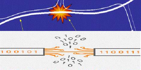
Figure 1: Packets being dropped in a congested network

There are many reasons for packet loss, the main cause being network congestion as you can see in the above diagram. Congestion results from applications sending more data than the network devices (routers and switches) can accommodate, thus causing an overflow of packets which results in some of the packets being lost. There are also other effects for congestion such as queueing delay and blocking of new connections.[1] For example on a video call between two systems, it is a real time function, if the network gets congested due to sending more packets than the network device can accommodate, then we will notice packet loss. The real time stream would lag and the quality of video will decrease and it can be observed that some packets were lost by noticing that video and the voice has skipped seconds of the real time stream. Another important role packet loss plays is in performance of network which greatly effects quality of service. Quality of service (QoS) is the idea that transmission rates, error rates, and other characteristics can be measured, improved, and, to some extent, guaranteed in advance. QoS is of particular concern for the continuous transmission of high-bandwidth video and multimedia information. [2]

In computer networks, network traffic measurement is the process of measuring the amount and type of traffic on a particular network. Previously a range of studies have been performed from various points on the internet. The AMS-TX (Amsterdam Internet Exchange) is one of the world’s largest internet exchange. It produces a constant supply of simple internet statistics. [3] This measurement capability also provides operators with greater visibility into the performance characteristics of their networks, thereby facilitating planning, troubleshooting, and network performance evaluation. Through this project I would do an experimental investigation of packet network performance and measure an approximation of how much packet loss can be observed through probability statistics. Packet loss is measured as a percentage of packets lost with respect to packets sent. In this document simulations are done and results are obtained to have result of this measurement and these results are vital as packet loss in network is of great importance since it effects QoS greatly.

Chapter 2: Aims and Objectives

Aims

The main aim of this project was to develop a simulation on MatLab for investigating packet performance and measure an approximation of packets lost in the simulation using statistical probability formulas.

Objectives

Research:

• To learn about simulation in detailed for transfer of packets from an end system to another end system in detail.
• To gain knowledge about packet loss in networks and how if effects the performance of the network.
• To gather adequate knowledge about MATLAB from https://matlabacademy.mathworks.com/. [4]
• To do background research on performance on networks.
• Carry out research on the formulas to be used.

Use of MATLAB:

• To keep track of the number of packets lunched and lost in the simulation
• To build simple model in MATLAB where packets are transferred from sender to receiver and packets are lost randomly with packet loss probability of 0.01.
• To build simple model in MATLAB where packets are transferred from sender to receiver and packets are lost randomly with packet loss probability of 0.001.

• Generate the simple transfer of model 10 times to have an accurate measurement on the performance of packets.
• To build a good state bad state model of transfer of packet from sender to receiver with probability ‘p’ being from good state to bad state and probability ‘q’ being bad state to good state.
• Generate the good state bad state model 10 times to have an accurate measurement on the performance of packets.
• To test the standard deviation of the performance of packets keeping Packet loss probability 0.01 and 0.001 and changing values of q alongside figuring out corresponding values of p.
• To do confidence intervals of the results obtained to have more accurate measurement of the performance of packets.

Use of Excel

• To produce graphical representation of the results obtained from simulation.
• Conclude and write my report based on my experimental investigation

Chapter 3: Background Research

Packets

A term first coined by Donald Davies, the person who developed the concept of packet switching in 1965 [5], a packet is a segment of data sent from one computer or device to another over a network. Whenever one computer is trying to send information to another computer or even when an internet user is browsing the internet, the communication between computer to computer and user to server (Internet service) is done through the transfer of packets between them. A packet contains the source (the address of the sender), destination (the address of the receiver), size (how big the packet is), type, data, and other useful information that helps packet get to its destination and read. Below is a breakdown of a TCP packet. Each packets are 32 bit in size. Another name for a packet is a datagram. Data transferred over the Internet is sent as one or more packets. The most common packet sent is the TCP packet. The other way to send packets is UDP, which is a connectionless protocol that has very few error recovery services and no real guarantee of packet delivery. Connectionless meaning, packets are placed in the network and the loss of packets cannot be tracked. The size of a packet is limited, so most data sent over a network is broken up into multiple packets before being sent out and then put back together when received. When a packet is transmitted over a network, network routers and switches examine the packet and its source to help direct its direction. During its transmission, network packets can be dropped. If a packet is not received or an error occurs, it is sent again. [6] [7]

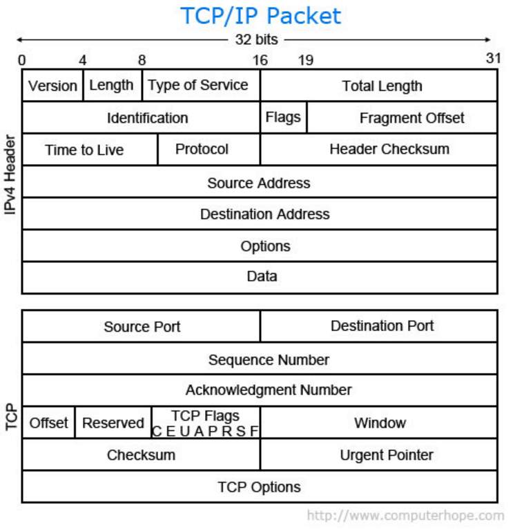
Figure 2: An Example of a TCP packet

Packet Performance

Packet performance also means network performance as network performance is always depended on the performance of packets. Network/packet performance refers to measures of quality of service of a network as seen by the user. There are many different ways to measure the performance of a network, as each network is different in nature and design. Performance can also be modeled and simulated instead of measured. In this project performance has been modelled and simulated using MatLab. [8]

As an average user of the internet would assume that good speed of the network is a good network performance benchmark. But speed is not everything when it comes to network performance. The ability of a network to support transactions that include the transfer of large volumes of data, as well as supporting a large number of simultaneous transaction is also a part of the overall picture of network load and hence of network performance. [11]

Measurement

Many internet service providers depend on the ability to measure and monitor performance metrics for packet loss and one-way and two-way delay, as well as related metrics such as delay variation and channel throughput.  This measurement capability also provides operators with greater visibility into the performance characteristics of their networks, thereby facilitating planning, troubleshooting, and network performance evaluation. When troubleshooting network degradation or outage, it is necessary to find ways to measure the network performance and determine when the network is slow and for what is the root cause (saturation, bandwidth outage, misconfiguration, network device defect, etc.). Through this experimental investigation of packet, it will be possible to come up to a conclusion about indicators which will put tangible figures to reflect the performance of the network. [9]

Quality of Service

Quality of Service (QoS) for networks is an industry-wide set of standards and mechanisms for ensuring high-quality performance for critical applications. By using QoS mechanisms, network administrators can use existing resources efficiently and ensure the required level of service without reactively expanding or over-provisioning their networks. [10]

What affects QoS?

There are 3 major network performance indicators and these are the factors that affect QoS. [9]

• Latency is the time required to transfer a packet across a network.
• Throughput is defined as the quantity of data being sent/received by unit of time.
• Packet loss reflects the number of packets lost per 100 of packets sent by a host.

From all these indicator this document will investigate elaborately on packet loss.

Packet loss

Packet loss occurs when one or more packets of data travelling across a computer network fail to reach their destination. [1]

Causes

Packet loss is typically caused by network congestion. When content arrives for a sustained period at a given router or network segment at a rate greater than it is possible to send through, then there is no other option than to drop packets. If a single router or link is constraining the capacity of the complete travel path or of network travel in general, it is known as a bottleneck, this is when packets are unable to be transferred. [1]

Packet loss can be caused by a number of other factors that can corrupt or lose packets in transit, such as Device (Router/Switch/Firewall/etc.) Performance. If the bandwidth (volume of information per unit of time that a transmission medium can handle) is adequate, there is still a possibility of the router/switch/firewall is not able to keep up with the traffic. Let’s take a scenario where the connection has been recently upgraded a link from 1 GB to 10Gb because traffic reports show that you were at full capacity during peak hours of the day. After the upgrade, your charts show the bandwidth going up to 1.5 GB, but you are still experiencing network performance issues. The issue could be that the device is not able to keep up with the traffic, and you have hit the maximum throughput your hardware can provide. The traffic is reaching the device, but the device’s CPU or memory is maxed out and not able to handle extra traffic. This results in packet loss for all traffic that is beyond the capacity of the box. [12]

Another reason for packet loss can be Software issues (bugs) on a network device. There are incidents when the software written for the network device is not perfect and there are still bugs in it. These network devices are extremely complex, and it is a matter of time before the user stumbles upon a bug. These bugs can cause new features to not work at all when deployed, or can go undetected for a while before noticing performance issues. [12]

Other reasons may include faulty hardware and cabling which lead to packets being dropped and Packet loss can also be caused by a packet drop attack which is due to the router disregarding packets because of its function of routinely dropping packets. [1]

Effects

Packet loss can reduce throughput for a given sender, whether unintentionally due to network malfunction, or intentionally as a means to balance available bandwidth between multiple senders when a given router or network link reaches nears its maximum capacity. [1]

When reliable delivery is necessary, packet loss increases latency due to additional time needed for retransmission. Assuming no retransmission, packets experiencing the worst delays might be preferentially dropped resulting in lower latency overall at the price of data loss. [1]

During typical network congestion, not all packets in a stream are dropped. This means that undropped packets will arrive with low latency compared to retransmitted packets, which arrive with high latency. Not only do the retransmitted packets have to travel part of the way twice, but the sender will not realize the packet has been dropped until it either fails to receive acknowledgement of receipt in the expected order, or fails to receive acknowledgement for a long enough time that it assumes the packet has been dropped as opposed to merely delayed. [1]

Measurement

Packet loss is measured by finding the probability of packet loss which is

• ‘LossPkt’= this is counter set to count the number of packets lost in the transmission
• ‘NormalPkt’= this is the counter set to count the number of packets that are sent normally/safely in the transmission without being lost.

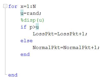
Figure 8: Code for Random Packet Loss

In figure 7 the code is displayed for which random packet loss can be observed for the number packets that are in the transmission as packets in. In this simulation for loop is used for all the packets that are in the transmission. Each packet is compared with the random number that has been generated and if the random number is less than packet loss probability which I had set at the start being “0.01” a packet would be lost in the transmission. If packet is to be lost then “LossPkt” counter increments by one if not “NormalPkt” is incremented by one.

Using values obtained from the simulation, the probability of packet loss from this simulation can be obtained, where pLoss= probability of packet loss. pLoss can be measured by dividing “LossPkt” by “N” which is total number of packets sent in the transmission.

The simulation of this transfer of packets is ran with different value of “N”, meaning different total packets in to the transmission. The reason for this is to investigate all types of data packets that would be at a particular time in this transmission. Firstly a huge number of packets are chosen, with “N=1000” as the parameter to the simulation. Then it was ran with different values of “N” such as 1000, 100 and 10. When 10000 packets are in the transmission it means there is huge traffic, it is expected to have more packet loss, 10000 packets would be times when the network at that point is very busy with many packet passing through that point and thus packet loss occur. For example when it is deadline time at university everyone is trying to use the intranet to submit their work and it would take them longer than usual to do it or not even get to do it and it fails, this is due to packet loss which is due to congestion in the network. Other times when 1000 packets are in the transmission is when there is high usage of their internet for example during the day at library internet is much slower than at night because it is peak time to study for students, due to high usage of internet at peak time students might experience the internet being slower than it is at night and this is due to network congestion and packet loss. For 100 packets, it is expected not lose too many packets. An example of this can be an internet call, sometimes user might experience that there is skip of words from the other side that is trying to communicate and this a result of packet loss. The user might also experience that the skipped word arriving much later than spoken, meaning it is not in real time. This means that there was packet loss observed by TCP but then it was recovered from lost packets. For 10 packets, it is expected that there should not be any loss of packets, as the number of packet in is very low. An example of 10 packets can be a text message sent from one computer to another. It is important to notice that if packets were lost for example when many users are sending messages to the same end system at same time, since the number of packets is so low, the effect of packet loss would be drastic. The text message might contain confidential information and might be lost in transmission and rerouted to unauthorized personnel. So the more the value of “p” from the simulation would mean there is more packet loss in the simulation of established packets in in and a low value of “p” would mean there is less packets loss in simulation with its respective packets in the simulation. A figure displaying the results obtained from the simulation can be found below in figure 8. Bar chart was chosen to display the value because bar chart would be able to display the difference of packets lost in regards to packets that are in the network at a particular time at a particular point. The difference can be easily distinguished looking at the bar chart.

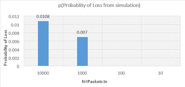
Figure 9: A bar chart showing Probability of loss from the simulation

The results obtained from simulation of different packets in can be found in figure 8. Figure 8 is displaying a bar chart. In this bar chart, for all the values of number of packets probes (N) (shown as the X axis) the corresponding packet loss probability is shown against the bar. The Y axis shows the probability of loss set as an input parameter for the simulation. The value of the loss probability from each simulation was determined as the (ratio packets lost in simulation) / (total packets in). As expected, the results show that for high numbers of probes, when 10000 packets were used, more packet loss was observed, and during times when a lower numbers of probes the packets were used, there may be as little as no packet loss observed. Obtaining a probability of loss of 0 means no packet loss was observed; this doesn’t mean that the packet loss probability was zero however.

Simulations ran with Packet Loss Probability of ‘0.001’

As mentioned in background theory the standard for packet loss probability on the internet is 0.001. It was mandatory to experiment the simulation with PLP (Packet Loss Probability) = 0.001.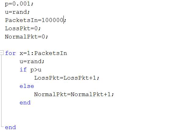

Figure 10: Changing P to 0.001

As you can see, the code for the simulation is the same as it was when ran with Packet Loss Probability of 0.01. The only two pieces of variables that is being updated here is “p” which is packet loss probability is being updated to 0.001 and “PacketsIn” to 100000. The simulation is ran and the results are obtained as you can see below in the table.

Figure 11: Results with packet loss probability of 0.001

As it can be noticed in the above figure that the results for 0.001 and 0.01 are very relatable. The main difference being the impact as it was expected, there is very less loss of packets and the values are very small for the measures and some calculations were not possible due to no packet loss being observed. The conclusion remains the same about this data as it was about the previous data.

Having a better measure of accuracy

In this section of the project and this document my main is to have a better measure of accuracy. This is done by running the same simulation 10 times and obtaining a grand average and then calculating its confidence interval. To calculate confidence interval the mean of the packets lost in the simulation is needed to be found. This can be obtained using the formula for mean when it comes to probabilities and this is known as expected value. The expected value can be calculated using “pLoss” which is probability of loss of packets from the simulation multiplied by the sample size “N” which in this case is total packets in.

Figure 12: Code for grand average of mean and standard deviation calculation

In figure 9 above, it can be noticed that arrays are introduced into the code as there are multiple simulation ran of the same code to find a grand average and confidence interval of packet loss. To find the Expected value it is important to take into account all the probability of loss of packet in each simulation and all these values will be hold in the array “pLossArray”. The other half of the code, standard deviation is introduced, standard deviation is necessary to find the confidence interval of the packet loss I am observing through these simulation. The formula for Standard deviation can be seen in the figure 9. Where “pLossArray” is used to divide by the total population which in this case is “N”, the total number of packets sent in the network.

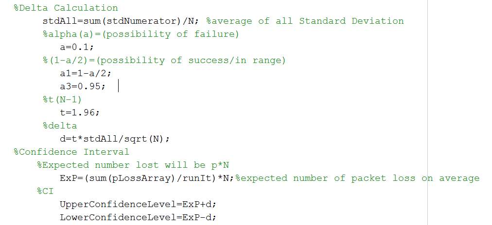
Figure 13: Code for Delta Calculation and Confidence Interval

In figure 10, the rest of the code needed to measure the accuracy of our result is displayed. Here the code is summing up the standard deviation obtained from the result to come up with the delta value. The delta value is the range (+ -) by which the sample mean (expected value) can vary. As there is always possibility of sampling error this measure of confidence interval was needed. Alpha (a) is the significance level where data can be wrong. And alpha is divided by 2 because of lower and upper boundary, so data can be wrong on either ends. The t value is obtained from t table for 95% and it is 1.96 [19]. Using all these values obtained from the simulation and knowing value of t from t table delta is calculated. As mentioned before the grand average of the mean is calculated before figuring out the confidence interval. The grand average (expected value of all 10 simulations) is calculated by summing all the “pLoss” or the whole “pLossArray” and dividing it by “runIt” which is total number of times the simulation has ran, the total number of times this simulation has been repeated is 10. The last part of the formula is adding and subtracting the delta value (d) from the grand average (ExP) to establish the confidence interval for the results obtained from the simulation.

Figure 14: results from multiple runs

As it can be observed from figure 11, the results that were obtained from multiple simulation using Packet in as the parameter to the simulation. The results obtained are much similar to the results obtained before for when simulation was ran once for each parameter value of N but this results is more accurate. As this is a grand average of 10 runs, it is possible that in the network at the certain time there are packets being lost from different sender trying to send packets to the same receiver. Due to congestion packets would be lost. Since we are measuring packet performance it is important to have an accurate measurement of packet loss, the reason why the simulation was ran multiple time. From this data table compared to figure 10 in last simulation it can be observed that in both as N, number of packet in (probes) are getting lower the probability of loss is getting lower also which again suggest that when there are high number of packets in the network packet loss is observed more. The main difference found in accuracy is that for the run of 100 packets in, now I have observed packet loss when ran multiple time but in the first simulation when ran once there was no packet loss observed for 100 packets in. in this table the values of mean and standard deviation for values of N is also introduced. Standard deviation portrays the spread of data, a high standard deviation would mean that the values are well spread out away from the mean and a low standard deviation would mean values are close to the mean. As the values of packets in decreases standard deviation is increasing which suggests that packet loss when sent in low numbers affects the performance of network more. Standard deviation is also used to calculate the Delta value for our values of packet in (N) to find the range by which the sample mean for given N can vary. As the standard variation increases the delta values also increases. The delta value is calculated to be used in calculating upper and lower confidence intervals. Confidence interval will give an accurate estimation by which my sampled mean can vary for the given data. The confidence interval for each values of Packet In can be found in figure 11.

Simulations ran with Packet Loss Probability of ‘0.001’

The same simulations was ran with packet loss probability of 0.001 and more accurate measurement of the results are displayed below in the figure.

As expected in the figure above it can be noticed that I have a more accurate measurement of random packet loss in a network with Probability of Packet Loss 0.001. In the previous figure when the simulation was ran once, there were no values for when N was 1000,100 and 10 but now 1000 and 100 have a value and there measurement are more accurate as the grand average of all simulations were taken into account.

Two state simulation of Network

In this part of the report, the report is moving onto a better representation of the computer network. Here the model of the network has two states, Good State and Bad State. Good State is when the network is not overloaded with packets, thus there is no congestion. This state of the channel is also known as the status of the network being in a good channel. Bad State is the network is overloaded with packet resulting in congestion and packet loss, this is when the network in a state where the status of the network is in a bad channel. The model for this simulation can be found in the figure below.

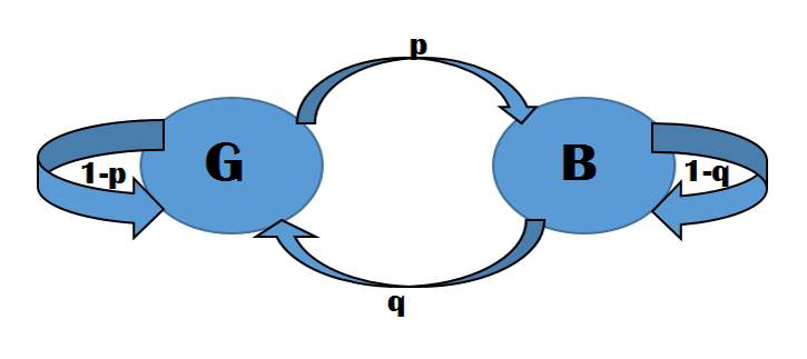
Figure 15: Model of a two state network

In the above figure the two states of the network is outlined. Where

• “G”= good state
• “B”=bad state
• “p”= probability of channel changing from good state to bad state
• “q”= probability of channel changing from bad state to good state
• “1-p”=probability of the channel remaining in good state
• “1-q”=probability of the channel remaining in bad state

This representation of computer network is better than random packet loss in the network which was done in the earlier simulation. The MatLab code for this simulation can be found in the figure below.

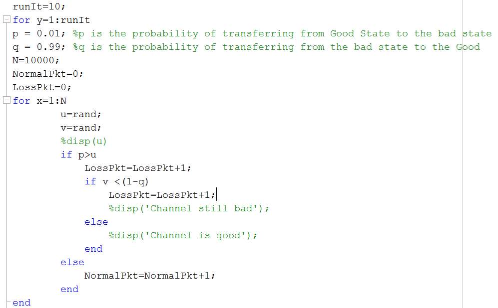
Figure 16: Good State Bad State Simulation Code

In the figure above the code for simulating good state bad state model is displayed. The same variables are used in this simulation as it was used for random packet loss model with a few new variables as it is a two state model. This simulation is ran 10 times to have a better accuracy of results with grand averages. In this simulation probes (packets in) are passed as N. The for loop is being used to run all probes through the network and as before the counter for packet loss and normal packets are added. In this simulation, the probability of packet transferring from good state to bad state is “p” which is 0.01, which is compared to the random number generated and if the value is lower than 0.01. The transfer of packets will move to bad channel and it will keep on losing packets with probability of “1-q” in bad state. The probability of packets transferring from bad to good state is “q” with 0.99 probability and the channel will then change to good and remain in good with probability of “1-p”. The standard deviation and mean formula used for this simulation is the same as before with arrays in the code as the simulation was ran 10 times. The results obtained from this simulation can be found in the figure below.

Figure 17: Results Obtained from Good State Bad State Simulations

As it can be observed from the figure above with the two state model the representation of the network is better than random packet loss model. Unlike the random loss model the standard deviation in these results for their respective probes (Packet in) is higher. This suggest that the spread of packet loss in the two state model is higher. Which results in the delta calculation of the measure by which mean can vary be to be higher also. This concludes that the two state model has larger confidence intervals than the random packet loss model. As two state model is a better representation of a computer network, the reason being congestion. As it can be seen in the figure above that when there is a high number of packets in the network more packets are being lost than expected as there is congestion in the network and the channel changes its state to bad and when in bad state/channel the network keeps on losing packets until the state of the network changes to good.

Keeping p (Loss) constant

In this section of the document I am trying to measure the changing values “p” which is the probability of the network changing from good state to bad state with its corresponding value of “q” which is probability of the network changing bad state to good state keeping p (Loss) constant to “0.01”. With this simulation keeping probability of packet loss constant to 0.01 different delta measures can be obtained for the same packet loss probability. As it is possible that at different times the probability of the network transferring packets from the bad state to good state is different depending on network congestion after the channel of the network has change from good state to bad state. The formula used to calculate “p” and “q” is:

• P(Loss)

  =pp+q

• Where P(Loss)= 0.01
• “p” is the probability of channel changing from good state to bad state
• “q” is the probability of channel changing from bad state to good state

The results for this simulation in the two state model was ran, the code remained the same as it was in the two state model section. The results obtained is in the figure below.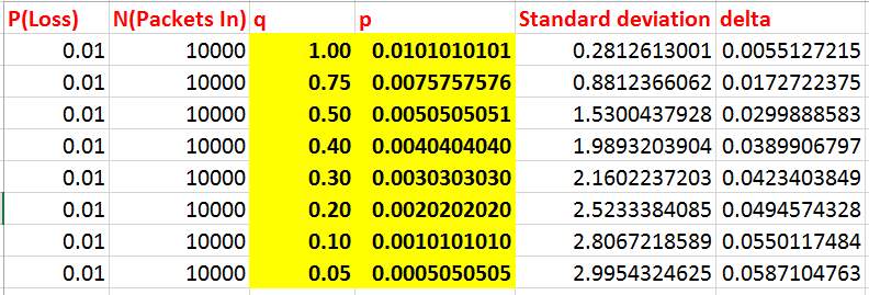

Figure 18: Changing values of q keeping P constant to 0.01

In the above figure, keeping P constant and using the formula mentioned earlier corresponding values of “p” were found by changing values of “q”. It can be observed that for the same number of packet loss in the 2 state model, as p becomes smaller loss happens more rarely. But when it does happen lots of packets are lost. The data in the table suggest that also, as you can see the lower p gets, q is getting lower also, and if you notice the last entry in the table, “q=0.05” meaning if the state of the channel changes to bad it will be very hard to change the state back to good as “q” is so low. So once the channel changes with this probability of p to bad state lots of packets will be lost being in the bad state. The table also suggest that the delta chance of which data can vary from the mean gets longer/bigger for the same packet loss probability.

Chapter 5: Discussion

Discussion

Further work

Chapter 6: Conclusion

Chapter 7 : My References

1. En.wikipedia.org. (2017). Packet loss. [online] Available at: https://en.wikipedia.org/wiki/Packet_loss [Accessed 16 Apr. 2017].
2. SearchUnifiedCommunications. (2017). What is QoS (Quality of Service)? – Definition from WhatIs.com. [online] Available at: http://searchunifiedcommunications.techtarget.com/definition/QoS-Quality-of-Service [Accessed 16 Apr. 2017].
3. En.wikipedia.org. (2017). Network traffic measurement. [online] Available at: https://en.wikipedia.org/wiki/Network_traffic_measurement [Accessed 16 Apr. 2017].
4. Matlabacademy.mathworks.com. (2017). MATLAB Academy. [online] Available at: https://matlabacademy.mathworks.com/ [Accessed 16 Apr. 2017].
5. En.wikipedia.org. (2017). Donald Davies. [online] Available at: https://en.wikipedia.org/wiki/Donald_Davies [Accessed 17 Apr. 2017].
6. Computerhope.com. (2017). What is packet?. [online] Available at: http://www.computerhope.com/jargon/p/packet.htm [Accessed 17 Apr. 2017].
7. White, G. (2017). How Do Packets Get Around? | Understanding Networks and TCP/IP | InformIT. [online] Informit.com. Available at: http://www.informit.com/articles/article.aspx?p=131034&seqNum=5 [Accessed 17 Apr. 2017].
8. En.wikipedia.org. (2017). Network performance. [online] Available at: https://en.wikipedia.org/wiki/Network_performance [Accessed 17 Apr. 2017].
9. Rogier, B. (2017). Network performance: Links between latency, throughput and packet loss. [online] Blog.performancevision.com. Available at: http://blog.performancevision.com/eng/earl/links-between-latency-throughput-and-packet-loss [Accessed 17 Apr. 2017].
10.  Anon, (2017). [online] Available at: https://technet.microsoft.com/en-us/library/cc757120(v=ws.10).aspx [Accessed 17 Apr. 2017].
11. Cisco. (2017). Measuring IP Network Performance – The Internet Protocol Journal – Volume 6, Number 1. [online] Available at: http://www.cisco.com/c/en/us/about/press/internet-protocol-journal/back-issues/table-contents-23/measuring-ip.html [Accessed 17 Apr. 2017].
12. Hurley, M. (2017). 4 Causes of Packet Loss and How to Fix Them. [online] Annese.com. Available at: http://www.annese.com/blog/what-causes-packet-loss [Accessed 17 Apr. 2017].
13. En.wikipedia.org. (2017). Expected value. [online] Available at: https://en.wikipedia.org/wiki/Expected_value [Accessed 18 Apr. 2017].
14. WhatIs.com. (2017). What is probability? – Definition from WhatIs.com. [online] Available at: http://whatis.techtarget.com/definition/probability [Accessed 18 Apr. 2017].
15. En.wikipedia.org. (2017). Standard deviation. [online] Available at: https://en.wikipedia.org/wiki/Standard_deviation [Accessed 18 Apr. 2017].
16. Itl.nist.gov. (2017). 7.1.4. What are confidence intervals?. [online] Available at: http://www.itl.nist.gov/div898/handbook/prc/section1/prc14.htm [Accessed 18 Apr. 2017].
17. M. Averill & Kelton, W. David (2006). Simulation Modeling and Analysis. Singapore: McGraw-Hill Book Co by Law. 112-132.
18. En.wikipedia.org. (2017). MATLAB. [online] Available at: https://en.wikipedia.org/wiki/MATLAB [Accessed 18 Apr. 2017].
19. Anon, (2017). [online] Available at: http://uregina.ca/~gingrich/tt.pdf [Accessed 18 Apr. 2017].
20. Anon, (2017). [online] Available at: http://www.eu.ntt.com/content/dam/nttcom/eu/pdf/services/network/ip-network-transit/sla-of-global-ip-network/NTTE_GIN_SLA_250210.pdf [Accessed 19 Apr. 2017].

Chapter 8: Appendix