Smart Energy Meter: Automated Meter Reading (AMR)

1.     INTRODUCTION

 

1.1 Smart Energy Meter

A Smart energy meter is an advanced energy meter that can measure the energy consumption of a consumer and at the same time provide added information to the utility by means of a two-way communication scheme [1]. Consumers are better informed and aware about their energy consumption, so that they can make better informed decisions when using energy. The need for manually billing the consumer by door-to-door visit is shifted to automatic online billing, which is practiced very commonly in a country such as India and hence SEMs become a great deal for saving manpower and time. This system that utilizes one-way communications to collect the data is referred to as automated meter reading (AMR) system. While the system that utilizes two-way communications with the ability to control and monitor the meters is referred to as advanced metering infrastructure (AMI) system. This combination of automatic reading and two-way communication is the reason why the meter is called ‘smart’ and is also the main difference between the traditional energy meter and a smart energy meter.

The idea of AMR technology is to read the meters automatically and accurately. The benefit of AMR is reducing the meter cost to the supplier and billing the customers with actual meter readings. In addition, AMR will increase the accuracy of the readings and it can allow frequent reading [2]. Smart meters are able to send the readings over communication lines and recognize their addresses and to activate/deactivate internal modules. To have that capability, AMR requires a specific infrastructure which would make it bidirectional. Such an infrastructure is called AMI. The communication medium in an AMI system must ensure the communication between the smart meters and the central computer at the service provider. The AMI network has the ability to register meter points, communicate into the customer premises, service connecting and disconnecting and other capabilities [3].

The communication structure can be wired like Power Line Communication (PLC) or wireless like Global System Mobile (GSM) and WiMAX. The chosen way must take into account the distances between the devices and the existing infrastructure [4]. GSM is a digital mobile telephony system that digitizes and compresses data before sending it. The main advantage of the GSM is its widespread use throughout the world and the use of subscriber identity module (SIM) cards to send short message service (SMS) messages. Another new technology that smart meters are using is the ZigBee communication. ZigBee is a low-cost networking standard. It is also low-power and wireless best suited for local coverage such as Home Area Networks (HANs). ZigBee is a key technology for the smart grid considering its automated controllability of appliances, ability to control devices, and lower installation and upgrade cost. ZigBee can offer meter-to-meter communication and remote monitoring ability of whole home conditions [5].

Smart meter is an important component of the smart grid. Detailed load flow can be provided by such meters to the distributers so they can manage the grid effectively. Other features like recording the power quality, detecting any unauthorized access to the meter and storage capability will all help and improve the grid. Smart grid is a type of electrical grid that intelligently responds to the behavior and performance of all electric power components in order to deliver electricity services efficiently. The smart grid delivers electricity from suppliers to the consumers by using digital technologies to save energy, reduce cost and increase reliability of the system. The smart energy meter that we propose to develop and are working on, is an attempt to effectively perform the above task and make energy affordable and accessible by all at all times.

1.2 Demand Response Management

Demand side management or Demand Response Management is an important utility in the future smart grid technologies for energy management, which provides support towards smart grid functionalities in various areas such as electricity market control and management, infrastructure construction, and management of decentralized energy resources and electric vehicles. By controlling the energy demand using the controllable loads, one can reduce the overall peak load demand, shift the load to off peak times thus reshaping the demand profile and thus reducing the overall cost which leads to increased grid sustainability. Efficient demand side management can potentially avoid the construction of an under-utilized electrical infrastructure in terms of generation capacity, transmission lines and distribution networks.

The smart metering devices in automatic metering infrastructure can be used to implement smart pricing, which is a unique characteristic of smart grid. This leads to cost-reflective pricing based on the entire supply chain of delivering electricity at a certain location, quantity and period. Smart pricing is used with demand side management, the customers’ energy usage can be controlled by real-time penalty and incentive schemes.

Demand side management also plays a significant role in electricity markets. The cluster’s central controller will be informed about the new load schedule to optimize the power consumption using Demand side management. After this the central controller places bids in the market such that the required loads be shifted. Profits made through this load demand side management will be reimbursed to customers of the cluster.

There are many demand side management algorithms which can used, but most of them are system specific strategies. Linear and dynamic programming are used for most of the techniques. These types of programs cannot handle large quantities of controllable loads as it has several computation patterns and heuristics. The primary objective of the algorithm presented in this project is reduction of system peak load demand and operational cost. In a smart grid, the demand side management strategies need to handle a large number of controllable loads of several types. Moreover, the loads usually have characteristics which spread over a few hours. Therefore, the algorithm suggested should be able to deal with all possible control durations of a variety of controllable loads.

2. FORECAST OF LOAD CURVE 

2.1 Objective

One of the objectives of this portion is to predict the amount of power available when the load is not at its peak and thereafter use this power to supply to consumers at the peak time. This process will effectively bring down the load curve.

For this purpose, prediction of off peak time is required, with which we can find when to store power efficiently. In order to predict the time of the day when the power consumption will go off-peak, we take the help of neural networks.

Neural Networks are tools in the field of control systems which are used to accurately represent any plant or model of a system. It is constructed to imitate the behavior of the human brain’s neurons’ way of working with analogous elements. Some of these analogies are:

1. Artificial Neurons

The units that represent the neurons of the brain. They form the fundamental unit of a neural network. They are crude approximations of the neurons found in the brains. They are mathematical constructs, but they can also be physical devices.

2. Neural Networks

They are network of neurons, which are also found in biological brains.

3. Artificial Neural Networks

They are a network of artificial neurons and hence can be viewed as an approximation to parts of real brains.

There are two types of uses of the typical neural networks problem:

1. Classification

Classification problems and their algorithms are used to predict the class labels (which are discrete in nature). Classification algorithm classifies a data after constructing a model based on an example data known as a training set and these values (known as class labels) in a classifying attribute and uses it in classifying new data of similar nature.

For example, predicting if cancer is malignant or benign, find T-shirt sizes using measurements like height and weight, etc.

2. Regression

Regression problems are used to predict the continuous valued function that “fits” into the given data. Estimate data which is about to occur (prediction) is a method under regression. Example for regression problems include, Stock Market Prediction of prices, temperature variation prediction, etc.

2.2 The Problem

In the given problem, the objective is to predict the occurrence of off peaks and on peaks data using previous values of the data. The data which is available is the 2010’s energy consumption data for a neighborhood of New York City, US. The data includes 3600 households’ consumption with primarily three types of consumers distributed among them:

1. High Consumers

High Consumers are those with the maximum amount of consumption of power in the neighborhood. They are roughly equal in number to the other two types of consumers (approximately 1200 households)

2. Base Consumers

Base Consumers are those with a moderate amount of power consumption in the neighborhood. The consumption levels are between high and low power consumers.

3. Low Consumers

Low Consumers are those with the least amount of power consumption in the neighborhood. Their number of households is also approximately equal to the other two types of consumers (approximately 1200 households).

2.3 Data Format

The data available is the hourly consumption data in the following format:

a. Date and Time of data

b. Electricity Consumption (total) (MW)

c. Gas Facility consumption (total)

d. Heating through Electricity (MW)

e. Heating through Gas consumption

f. Cooling with Electricity (MW)

g. HVAC Electricity (MW), this includes HVAC Fans Electricity Consumption

h. General Interior Lights Electricity consumption (MW)

i. General Exterior Lights Electricity consumption (MW)

j. Interior Application Equipment of Electricity (MW)

k. Miscellaneous Consumption (MW)

l. Water Heater: Water Systems (Gas consumption)

For the purpose of our predictive analysis we choose to use only the data for electricity and model only that in the simulation. Since our analysis is to determine the amount of data available during off peak to compensate for on peak, the overall electricity consumption (Column 2) is only taken into consideration for the 3600 households.

One can proceed in an alternative way by fixing a few of these columns as controllable devices. The objective then would be to determine which devices should run during peak and off-peak times in order to flatten the load curve and reduce the load demand. But in that case a rough guestimate of the usage of corresponding devices needs to be figured out using tools of neural networks.

2.4 Time Series Modelling

We use a technique in regression known as time series modelling to predict the data for the future. This data is predicted with the help of data from the past of the inputs.

In the case of our particular modelling, we use the data of the past four weeks to determine the value of predicted consumption. The data taken in the past four weeks is from the same hour of the same day every week. This is because consumption on a particular day of the week will be similar throughout the year. For example, the consumption in weekends will be very different from the consumption in weekdays. In weekends consumption will be more in residential areas than weekdays.

Hence the function for our prediction algorithm becomes:

y(t)=f(y(t-168),y(t-336),y(t-354),y(t-672))

(1)

Here 168 indicates 24*7 hours (exactly 1 week in hours). The training is done in two ways and their efficiency is determined. The two ways are:

a.       Levenberg Marquardt Training

b.       Adaptive Neuro Fuzzy Interface System Algorithm

2.4.1 Levenberg Marquardt Training

It is also known as Damped Least Squares training method. It is used to solve nonlinear last squares problems, which are used to fit a set of observations with a model that is non-linear in unknown parameters. It is used in some forms of nonlinear regression. It is used in many software applications for solving curve-fitting problems that are generic. However, as for many of the same fitting algorithms, this algorithm finds only one local minimum, which need not necessarily be the global minimum. Levenberg-Marquardt algorithm is an extension of gradient descent and an interpolation of Gauss-Newton Algorithm (GNA). The LM is said to be more robust than GNA. This means that in many cases it finds a solution even if in the initial iteration, the starting point is very different from the final minimum (either in state space or in definition of minima). LM Algorithm is said to be slower than GNA in complex problems. LM Algorithm can be seen as GNA when the objective function’s subset is minimized or approximated using a model function. The primary application of this algorithm is the least-squares curve fitting problem, given a set of m empirical data pairs (xi, yi) – of independent and dependent variables, the parameters β of the model curve f(x, β) is found out so that the root mean square deviation is minimized:

β=argmin∑[yi-f(xi,β)]2

(2)

From Gauss Newton Algorithm, we can approximate the Hessian by:

H=JTJ

(3)

The next iteration of x can be found using the following formula:

xk+1= xk-JTxkJxk+ μkI-1JTxkv(xk)

(4)

The data set was divided into two datasets for training and checking. The neural network was constructed with 2 hidden layers with 10 nodes each as this configuration was found to have the least error in training. The data was trained to yield the resulting neural network. The check data was then used to determine the error in training, the results of which are the following:

Mean Squared Error = 0.1940.

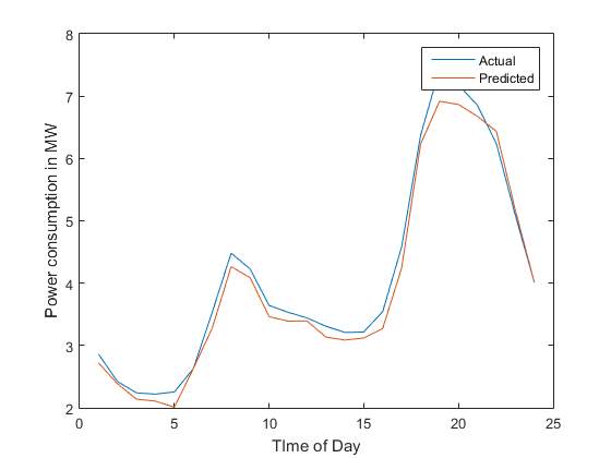
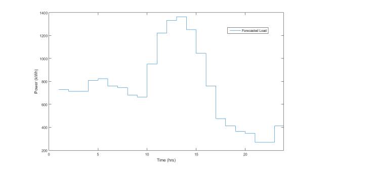
Figure 1. Forecasted Load

The figure 1 represents the predicted vs actual power consumption values. The predicted values are in red. The neural network appropriately models the peaks and crests in the original data.  The graphs on the next page, represent the training, the validation and the checking data and also the corresponding error.

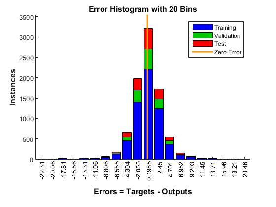
Figure 2. Error Histogram

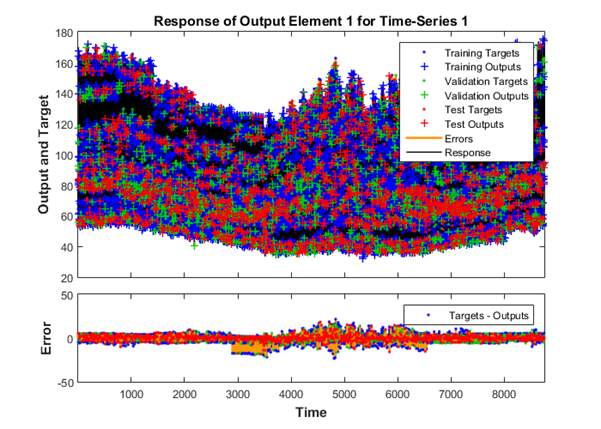
Figure 3. Response of Output Element 1

2.4.2 ANFIS

ANFIS stands for Adaptive Neuro-Fuzzy Inference System. It is a hybrid neuro-fuzzy technique that brings learning capabilities of neural networks to fuzzy inference systems. The learning algorithm tunes the membership functions of a Sugeno-type Fuzzy Inference System using the training input-output data.

Assume that the fuzzy inference system has two inputs x and y and one output z. A first-order Sugeno fuzzy model has rules as the following:

Rule1: If x is A1 and y is B1, then f1=p1x+q1y+r1

Rule2: If x is A2 and y is B2, then f2=p2x+q2y+r2

Usually a bell function is used to determine the truth value of each rule.

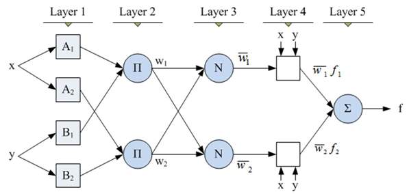
Figure 4. ANFIS Neural Network

 

Layer 1:

O1, i is the output of the ith node of the layer I. Every node i in this layer is an adaptive node with a node function O1, i = µAi (x) for i = 1, 2, or O₁, i = µB_i−2(x) for i = 3, 4. x(or y) is the input node i and Ai (or Bi−2) is a linguistic label associated with this node. Therefore O1, i is the membership grade of a fuzzy set (A1, A2, B1, B2).

Typical membership function:

μAx=1/(1+x-ciai2bi)

(5)

a_i, b_i, c_i is the parameter set.

Parameters are referred to as premise parameters.

Layer 2:

Every node in this layer is a fixed node labeled Prod. The output is the product of all the incoming signals.

O2,

i= wi= μAi(x)μBi(x)

i = 1, 2    (6)

Each node represents the fire strength of the rule. Any other T-norm operator that perform the AND operator can be used.

Layer 3:

Every node in this layer is a fixed node labelled Norm. The i^th node calculates the ratio of the i^th rule’s firing strength to the sum of all rule’s firing strengths.

O3,

i= wi= wiw1+ w2

i = 1, 2     (7)

Outputs are called normalized firing strengths.

Layer 4:

Every node i in this layer is an adaptive node with a node function:

O4,

1= wifi= wi(px+ qiy+ri)

(8)

w_i is the normalized firing strength from layer 3.

{p_i, q_i, r_i} is the parameter set of this node. These are referred to as consequent parameters.

Layer 5:

The single node in this layer is a fixed node labelled sum, which computes the overall output as the summation of all incoming signals.

A forward and backward pass technique is used for the learning Algorithm. In the forward pass the algorithm uses least-squares method to identify the consequent parameters on the layer 4. In the backward pass the errors are propagated backward and the premise parameters are updated by gradient descent.

The neural network was generated using the genfis function and the similar to the above method training and checking dataset was constructed. The neural network was trained using the training Dataset and then the error determined using the checking dataset.

Following results were obtained:

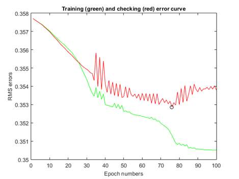
Figure 5. Training and checking error curve

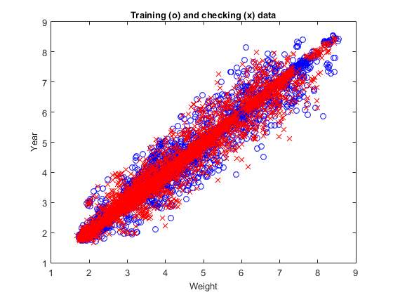
Figure 6. Training and checking data

Once the prediction of data is done the peak and off peak time can be calculated by finding the average power consumed in that day. When power consumption is less than average then off peak and vice versa. The area under the graph in peak is equal to the area under the graph in off peak. So energy consumption can be balanced to get a flat load curve.

3. DEMAND RESPONSE MANAGEMENT

Demand Response programs have been around for decades and have proven to be an effective means for utilities to manage system peaks by controlling customer loads. For residential consumers, these programs traditionally entailed the direct load control of large appliances at the home such as air conditioning systems, hot water heaters, and pool pumps. For the most part, these were one-way systems based on signals sent via pager, power line communications, energy management system, or telephone to the controlling devices to temporarily turn off or cycle the desired appliance during peak conditions. The utility benefitted from a better ability to manage demand and supply, while the customer benefitted from financial incentives for program participation. This approach proved to be an effective demand control solution and continues to work well today. But now, for an even brighter tomorrow, the need for a smarter grid arises. With this advent comes the requirement for a basic tool of energy measurement and management, i.e. a Smart Energy Meter (SEM).

Demand Response Management is managing the power consumption after understanding the consumption pattern to better enable efficiency and power consumption without overshooting the cost much. Since Electric energy cannot be stored easily, it is always possible to advise the consumer on their consumption patterns. The main aim would be to match the actual power consumption pattern to the ideal power consumption pattern (that is usually decided based on price). In conclusion we can say that demand response capability does not try to control the utility or power generation, transmission or distribution, but rather the consumption (or the utilization) patterns of the consumer itself.

In [11], the algorithm given to implement load shifting in demand side management was a linear programming algorithm. Linear Programming is used to solve simple programs               that involve optimizing a function. Optimizing a function usually involves either maximizing or minimizing the function. Usually the technique is used to solve linear relationships between input parameters. The problem for evolutionary algorithms, which will be used in this project, is generally non-linear in nature. The initial approach was of simple linear programming but this was discontinued because of the complex nature of the problem.

The function that is required to be optimized is known as a “fitness function” or an “objective function”. The function will be a representation of our objective of improving the efficiency of power consumption while trying to reduce the bill incurred on the consumer.

In Linear Programming the technique for optimizing the function is subject to linear equality or inequality rather than a complex nature (of a higher degree of complexity). The region of solution is a set defined as the intersection of planes that divide the three dimensional Euclidean space which are finite in number and are defined by a linear inequality. The objective function in this case is a real valued linear function. The algorithm finds the smallest value of the function (in our case).

In [12], Linear Programming is used in Residential load and Energy Management in Residential load where overall cost and Peak to Average Ratio (PAR) is minimized. Monotonic optimization based DSM strategy is proposed in the next paper [13], mathematical modeling of the centralized renewable energy source has been done. So this problem is with respect to renewable energy sources to demonstrate the optimal utilization of loads of such nature.

Electrical Power Distribution involves transfer of electricity from high-voltage transmission systems and delivers it at much lower voltages to the consumers. Since this system is of complex nature, distribution system overloading phenomenon might occur. It is when there might be a case of overloading of feeder or fault taking place in the distribution line. The supply could be provided through alternate paths to the consumers (through other feeder path) which has the adequate power supply required for this purpose. This problem is overcome with a strategy provided in [14]. The algorithm provided which checks the priority of appliance and then shut that particular appliance down to avoid distribution system overloading. As an example, large penetration of electric vehicles and its effect is also seen in the paper. Another aspect of stopping appliances is given in [15]. This technique is an Optimal Stopping Rule based appliance scheduling scheme. This is one of the fundamental ideas for this project.

In this technique, the algorithm gives the time when the price is low for the appliance to be shut down. What we are trying to achieve in load shifting demand side management is similar to this. A primary disadvantage, however in this is that the algorithm won’t be able to handle large power appliances nor can it handle large number of appliances.

Demand Side Management has usually employed various techniques to accomplish better handling of the load from the load curve of the system. Common methods include:

1. Peak Clipping

2.  Load Shifting

3. Valley Filling

4. Flexible load shape

5. Strategic Conversation

6. Strategic Load growth

Load Shifting is the technique employed to perform demand side management technique. In this technique, load shifting is done from on-peak to off-peak [10]. The proposed was a DSM strategy based on load shifting technique. Several types of large number of appliances are considered in this work to show the effectiveness of the proposed algorithm. In [10], the load shifting problem is solved using GA to reduce the cost and PAR. We solve the same problem as in [10]. Implementation of the GA is done on the utility side and is uploaded once a week in the AWS (since forecast of load is done for past 4 weeks) and can be calculated for an entire week at a time.

3.1 DSM Algorithm

This report presents a day-ahead demand side management (DSM) strategy for the future smart grid. It uses load shifting strategy that instructs the central controller of the smart grid. Objective of the demand side management could be maximizing the use of renewable energy resources, maximizing the economic benefit, minimizing the power imported from the main distribution grid, or reducing the peak load demand. The strategy is to design an objective load curve in accordance to the objective of the demand side management. This algorithm tries to bring the actual load curve as close to the objective load curve as possible. That is, say the objective of the demand side management strategy is to minimize the utility bill, the objective curve chosen will be such that it is inversely proportional to the electricity market prices. Therefore the algorithm receives the objective load curve as an input and calculated the desired load control to get the load curve as close as possible to the objective load curve. Therefore, the proposed algorithm is flexible in that it is completely independent from the criteria used to generate the objective load curve.

The demand side management is carried out at the beginning of the predefined control period. Then, the control actions are executed in real-time based on the results. This system uses the communication capability of the smart grid. Whenever the customer presses the ON button of an appliance a connection request is sent to the demand side management controller. The controller then responds based on the calculation it has done to optimize the load curve. The reply is either the connection permitted or a new connection time.

3.2 Problem Formulation

The proposed strategy schedules the connection time of shift-able load so as to bring the load curve as close as possible to the objective curve. The load shifting technique is formulated as follows

Minimize

∑t=1NPloadt-Objectivet2

(9)

where

Objective(t) is the value of the objective curve at time t,

Pload(t) is the actual consumption at time t.

The Pload(t) is given by the following equation:

Pload(t) = Forecast(t) + connect(t) – disconnect(t)   (10)

Where,

Forecast(t) is the forecasted consumption at time t,

Connect(t) and Disconnect(t) are the amount of loads connected and disconnected at time t respectively during the load shifting.

 

Connect(t) is made up of two parts: the increment in the load at time due to the connection times of devices shifted to time t, and the increment in the load at time t due to the device connections scheduled for times that precede t. It is given by:

Connectt=∑i=1t-1∑k=1DXkit.P1k+∑l=1j-1∑i=1t-1∑k=1DXki(t-1).P1+lk

(11)

Where,

Xkit

is the number of devices of type k that are shifted from time step i to t,

D is the number of device types,

P1k

and

P1+lk

are the power consumptions at time steps 1 and (1+l) respectively for device type k,

j is the total duration of consumption for device of type.

Similarly, Disconnect(t) also consists of two parts: the decrement in the load due to delay in connection times of devices that were originally supposed to begin their consumption at time step t, and the decrement in the load due to delay in connection times of devices that were expected to start their consumption at time steps that precede t. The Disconnect(t) is given by the following equation:

Disconnectt=∑q=t+1t+m∑k=1DXktq.P1k+∑l=1j-1∑q=t+1t+m∑k=1DXkt-1q.P1+lk

(12)

Where,

Xktq

is the number of devices of type k that are delayed from time step t to q,

m is the maximum allowable delay.

The number of devices shifted cannot be a negative value.

Xkit>0 ∀ i,j,k

(13)

The number of devices shifted away from a time step cannot be more than the number of devices available for control at the time step.

∑t=1NXkit≤Ctrlable(i)

(14)

Where,

Ctrlable(i)

is the number of devices of type k available for control at time step i.

The demand side management problem has characteristics such as, connection times of devices that can only be delayed and not brought forward, which can be expressed as

Xkit=0 ∀ i>t

(15)

Usually the contract has a maximum permissible delay for the devices agreed upon between the consumers and the suppliers beforehand

Xkit=0 ∀ t-i>m

(16)

Where,

M is maximum permissible delay to the load.

3.3 Proposed Algorithm

The demand side management algorithm proposed for future smart grid needs to have the ability to process a huge number of controllable devices of several types. Moreover, each of controllable device has different consumption characteristics which has its execution time spread over few hours. Therefore, the designed algorithm should be able to handle these complexities. Both linear programming and dynamic programming cannot adequately handle these complexities. Evolutionary computation algorithms have several advantages as compared to other algorithms besides also getting the optimal results. .Hence, in this paper, a heuristic based evolutionary algorithm is proposed, and has been developed to solve the problem.

The proposed algorithm not only adapts the heuristics in the problem easily but also provides an efficient and cost effective solution to the problem. The flexibility in constructing and developing the algorithm is one of the major advantages in this algorithm which cannot be afforded by any other conventional approaches. This flexible nature of evolutionary algorithm allows one to implement features that can model load demand patterns based on the day to day consumption pattern to minimize the inconvenience caused to the consumers. For example, Hair dryer is usually used in the morning whereas vacuum cleaner can be used anytime in the day. So, the algorithm can shift the Hair dryer as early as possible and shift the vacuum cleaner to a later part of the day. Priorities can also be given to the load so the time allocation can be done according to the priority of the load. Though this feature is not implemented in this project but can be implemented in the future. Another main advantage of the proposed algorithm is the ability to handle large number of controllable devices of several types. More the size of the problem, more will be the size of the chromosomes but the problem overall remains the same.

The maximum number of possible time steps can be found using the following equation:
N=(24-m×m+∑n=1m-1n)×k

(17)

Where,

k is the number of different types of devices.

Chromosomes of the evolutionary algorithm represents the solution the given problem. In this project, two chromosomes are taken. One is taken as array of number each representing the time to which the load is to be shifted. The other is the number of devices of each type to be shifted. The length of the chromosome is directly related to the types of devices. A population of 200 is initialized by taking random value between the upper and lower bounds of the gene.  A fitness function is chosen such that the algorithm achieves a final load curve as close to the objective load curve as possible, which is given as follows

Fitness=11+∑t=124Ploadt-Objectivet2

(18)

The following are the steps involved in minimizing the fitness function using genetic algorithm

1.                Initialize t=0.
2.                Randomly initialize the population which represents the patterns of appliances.
3.                Evaluate the fitness
4.                Apply the steps of genetic algorithm to the population
5.                The children population is obtained
6.                Choose the pattern from the population with the best fitness
7.                Check all the appliances status in chromosome
8.                Iterations=1, go to step 3
9.                Till either of maximum iterations or maximum tolerance is achieved.

In this process, new population of chromosomes are produced from existing population in every iteration by genetic operators, i.e. crossover and mutation. The crossover rate must be large enough to ensure faster convergence of the solution but a very high crossover rate may result in loss of good solutions from previous generations, and stop the algorithm with premature convergence. Best cross over rate (i.e., 0.9) and mutation rate (i.e., 0.1) were found experimentally for this problem. A tournament based selection is used for reproduction. The termination of the algorithm is done when the maximum number of generations (i.e., 500) is reached or when the magnitude in the change in fitness value does not vary more than a tolerance limit (i.e.,

10-10

) for several (i.e., 50) subsequent generations.

Figure 7. Forecasted Load Curve

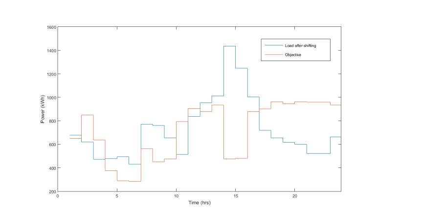
Figure 8. Objective and Final Load Curve

 

 

3.4 Results

Area	Cost without DSM (Rs.)	Cost with DSM (Rs.)	Percentage Reduction (%)
Residential	230290	213950	7.0957

 

 

 

 

4.      MODEL OF RESIDENTIAL LOAD

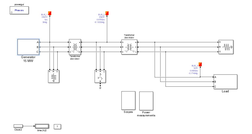
Figure 9. Model of Residential Load

 

4.1        The Generator

It is modelled similar to a Diesel Generator and the generating machine is simulated as a Synchronous Machine. It takes two inputs from the user, firstly the Output of the Diesel Engine Governor (Pm) that is controlled on the basis of the rotor speed (wm) and the reference speed (wref)  and secondly the Field Excitation energy (Vf_) which is provided by the machine itself, it being a self-excited field generator (Stator Voltages Vd and Vq). The power factor is assumed to be 0.16p.u.

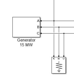
Figure 10. Generator Model

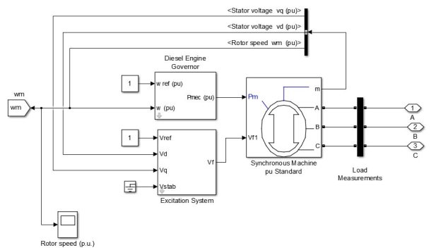
Figure 11. Inside the Model of generator

 

4.2        Isolation Transformer

Since the generation is simulated nearly to be 25kV and at the distribution it is transformed to 600V from 25kV directly, the generating transformer is assumed to be only an isolation transformer and not a LV-HV transformer.

4.3        Distribution Transformer

It is high to low transformer with the voltage ratings of the machine being (25kV/600V) at 20MW rated Power. The other parameters for both the transformers like winding resistance, inductance and the magnetizing inductance have been faithfully entered in the parameters table.

4.4 The load

This block is considered one of the most imporatant block with respect to the operation and the closed loop regulation of the Diesel Generator. This block produces the output of the sequential voltages Vd and Vq which are used to excite the Field winding coil of the generator. The Asynchronous Machine shown in this Load block is the linked duplicate of the same machine which is used for electricity generation as a Diesel Generator. These both are linked together just to make the model more cleaner and easily understandable. On exploring each block inside the load model the operation can be fully understood. The evaluation of some important variables has been defined in this section.

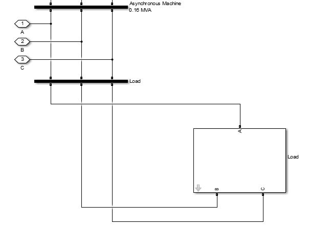
Figure 12. Model of Load

An intermediate variable V1 is created by using the following equation:

V1= ⅓(Vab- a²*Vbc), where Vab and Vbc are the respective instantaneous line voltages. From this V1, a variable d_theta is subtracted, to obtain the Stator voltages Vd (Direct Component) and the quadrature component(Vq). D_theta is obtained from the mechanical model of the machine and is dependent on the shaft input power and the rotor speed.

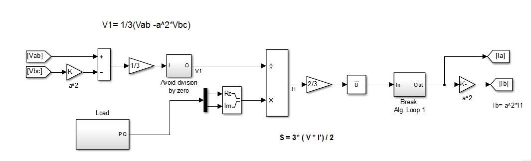
Figure 13. Simulation of load

From the load consumption data of our dataset the hourly averaged active power (P) is obtained. The other input of the multiplier ‘Product1’ is (

1/cos2θ

-1) which then gives us the hourly averaged reactive power (Q) as the output and thus the bus P and Q are obtained this way.

Ia and Ib are calculated by using the equations

S=3*V*I’

where S is the total power, I’ is Ia conjugate and V is V1. This Ia and Ib values are then sent to the controlled current source and hence based on our predicted dataset the current can be controlled in the AC bus.

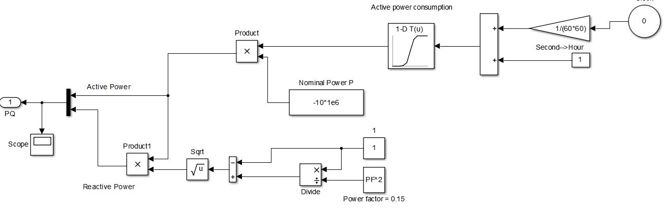
Figure 14. Simulation of connection of load to grid

Other than this, the product of the values of the Speed and Torque sensors help in determining the output electric power. The efficiency is assumed to be 99.46%.

 

 

5. CIRCUITRY

DC Regulated Power supplies of +12V and -12V are required for providing bias voltage to the various circuits. If the power supplies are made manually, the circuitry would be:

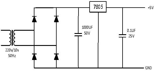
Figure 15.

In this circuit, a voltage of +5V would be required to drive the switches.

For the +12V and -12V bias voltage, the circuit would be:

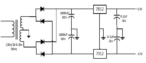
Figure 16.

 

5.1 Current Sensor

For current measurement, we would use Hall Effect current sensor:

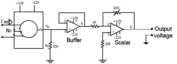
Figure 17. Circuit of Current sensor

A current of I(A) in power network is converted into ± 5V range. These current sensors provide galvanic isolation between high voltage power circuit and the low voltage control circuit and require a nominal supply voltage of the ±12V to ±15V. For a chosen primary turns (N_P), the conversion ratio of current sensor is 1000:1 and the output resistance of the current sensor is taken as 100 Ω. The voltage input to the buffer circuit is calculated by the equation

     (19)

Thus the voltage is scaled properly with the scalar circuit.

5.2 Voltage sensor

Voltage measurement is done with the help of AD202JN isolation amplifier. The AD202JN is an isolation amplifier in the present experimental setup the power circuit voltage which is in the range of ±500 V is converted into ±5V range. The voltage at the output of the isolation amplifier is

    (20)

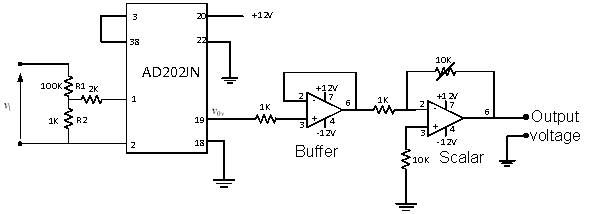
Figure 18. Circuit of voltage sensor

 

5.3 Raspberry Pi

The basic elements of a smart meter’s energy measurement front end are sensors, an analog-to-digital-converter (ADC), and the algorithms used by a dedicated MCU (Micro controller unit) or the meter’s host processor to interpret the raw data. The MCU can be an Arduino or a Raspberry Pi.

The Raspberry Pi is a series of small single-board computers developed in the United Kingdom by the Raspberry Pi Foundation to promote the teaching of basic computer science in schools and in developing countries.

The Raspberry Pi consists of digital input/output pins (called GPIO pins) which can be used for reading digital logic signals or for giving output of digital logic levels. The outputs are of a very low voltage range and a very low current range, because of which one can use LEDs to get signals and help understand outputs.

The GPIO pins are used to take input from the sensors for measurement of Voltage and Current which will reciprocate to the real time power in the system.

This real time measurement of power is stored in the internal memory of the Raspberry Pi and is used to forecast future data and also used to flatten the load profile of the system.

The Raspberry Pi GPIO pins are accessed by the GPIO module in python. It works very similar to a microcontroller like Arduino where in the pins can take the voltage level of the analog sensors that can translate to the measured value of the voltage or current.

The Raspberry Pi can take a maximum voltage of 3.3V in its GPIO pins. Care should be taken to ensure that the voltage levels are falling within the range for GPIO when coming from the sensors.

5.4 AWS Instance

An AWS instance is a part of Amazon Web Services initiative by amazon.com. It offers cloud computing platforms. These services include Amazon Elastic Compute Cloud (or the EC2) which is used in the project for communication from utility to smart meter. This EC2 service can be protected with a suitable ID and password also. Amazon markets AWS as a service capable of large computing capacity, sometimes faster than an actual physical server farm. An EC2 server is runs a LINUX based operating system which has certain essential software packages already installed like Python, PHP and MySQL etc.

An EC2 instance of AWS is run for the prototype. A file containing the details of:

1.                How many devices are to be shifted of each of the controllable devices category?
2.                From which time and to which time the operation of the devices is shifted.

The details are stored in a CSV file for the best iteration as decided by the heuristic optimization. This file can be transferred from a Windows system through WinSCP software. If the user uses LINUX on the utility end, simple terminal commands can be used to transfer the CSV file.

6. CONCLUSIONS

A self-sufficient RPi based smart energy metering system is suggested with the DSM capabilities. The following were found to be the amount of expenditure saved by applying Load Shifting technique to change consumption pattern of the consumer.

Area	Cost without DSM (Rs.)	Cost with DSM (Rs.)	Percentage Reduction (%)
Residential	230290	213950	7.0957

The graphs provided in results conclude that the objective function is matched with the power consumption, thereby proving that the method of using an evolutionary algorithm (in this case the Genetic Algorithm) works successfully.

7. FUTURE OBJECTIVES & IMPROVEMENTS – VEHICLE TO GRID SYSTEM

In the future the data of the predicted load could be integrated with the simulations of the actual power system, mostly distribution system. Further, the dynamic model of electric vehicles could be added to the same to obtain an even accurate efficiency values of the system, thereby making electricity more affordable and accessible by all.

Although, the main disadvantage with Electric Vehicles is the amount of time they take in getting charged and with the increase in the popularity of such vehicles, the “range-anxiety” is now very gradually being substituted by the “charging-anxiety”. Only a couple of minutes are required to fill up a diesel or gasoline engine car at a filling station with sufficient fuel to run for about 400kms, costing about 2500 bucks. But, to travel the same distance in a small electric passenger car would need charging a typical 10kWh battery that is used to power the vehicle, atleast 3 times costing not more than Rs. 300 in total with electricity priced at 10 rupees per unit.

There are three types of charging facility available for electric vehicles:

The Level 1 consists of Single Phase (AC) using grounded receptacles as used in most of the domestic appliances. This typically means a 15 Amps current at 240 Volts delivering a maximum of 3.6 kW of power. The EV can even include a standard domestic power cable for connecting the EV to a domestic socket outlet or a Level 1 charging station.

The Level 2 delivers up to a maximum of 33 kW of electric power from a Three Phase (AC) source of 415V at up to a very high 80Amps of current. The J1772 standard has been described by the Society of Automotive Engineers – SAE to cover the connector at both ends as well as the charging cable used in applications for this level, for safety purposes. These cords/cables are connected permanently to the Level 2 charging point rather than to the EV. This type of connector is also called a coupler.

The Level 3 refers to the Direct Current (DC) charging, or alternatively called “fast charging.” To minimize the charging times for these EVs this type of chargers supply currents as high as 400 Amps and at voltages as high as 600 Volts DC, delivering a maximum power of 240kW. This type of high power transfer undoubtedly decreases the charging time of EVs drastically but on the same time lifts up the minimum safety requirements needed for this to be safe for public use. SAE J1772 Hybrid coupler and the Japanese CHAdeMO. are some of the commercial standards used in this industry.

In this system, level 3 chargers is preferable as the amount of time to charge is also important. If it takes too long to charge then there won’t be any time to take energy from the vehicle to grid. In this type of charger the output is directly DC. For a charging station this type of output is preferable as the converters can be designed for public use, whereas for personal charging stations these converters will be very costly.

In modelling, there are two ways of approaching the simulation.

The first method is to consider only one type of vehicle system. This one fixed type of vehicle system will consume a fixed amount of power. In this we allot a fixed percentage of usage time and a fixed percentage of free time. Usage time refers to the time when V2G is active and free time is a percentage of time when V2G is not in use i.e. a consumer might be using the vehicle. A common example adapted is 80 – 20 rule. 80% of the day is used for V2G and 20% of the day is free time.

The second method will be to model different scenarios for a percentage of the total cars available. Here V2G has two functions. Controls the charge of the batteries connected to it and uses the available power to regulate the grid when an event occurs during the day. The block implements five different car-user profiles:

• Profile 1: People going to work with a possibility to charge their car at work. For eg. 35% of the cars are of this profile.
• Profile 2: People going to work with a possibility to charge their car at work but with a longer ride. For eg. 25% of the cars are of this profile.
• Profile 3: People going to work with no possibility to charge their car at work. For eg. 10% of the cars are of this profile.
• Profile 4: People staying at home. For eg. 20% of the cars are of this profile.
• Profile 5: People working on a night shift. For eg. 10% of the cars are of this profile.

This project suggests that a conventional smart energy meter to be replaced with the RPi prototype suggested in this report. This is a problem for the present, but will eventually become easier to deal with in the future. From RPi 3 onwards, an inbuilt Wi-fi module is provided. So it is not necessary to give the energy meter an Ethernet connection also. The Wi-fi module will do the collection of the necessary information for load shift at the beginning of the day from the AWS instance.

Security and Privacy should also be included in this project. For example, a protected server can be created instead of an EC-2 instance of AWS. This way, the consumption details of the consumer can be kept private protecting their privacy. A username and password might be provided for a particular household in order to check the consumption pattern should they need to.

The whole facility can also be provided in an Android/iOS/Windows application which could help the consumer access their consumption pattern remotely if needed.