What Factors May Influence Uninsured Rates in the United States?

Table of Contents

Click to expand Table of Contents

1. Introduction…………………………………………1-6

2. Collection of Data …………………………………….6

3. Independent variables “predictors” …………………………..6-7

4. Descriptive analysis……………………………………8

4.1. Total U.S. states statistics……………………………..8

4.2. Southern States Statistics ……………………………..9-10

4.3. northern states statistics………………………………10-11

5. analysis (Regression)…………………………………..11

5.1. preliminary assessments………………………………11-13

5.2. correlation matrix:………………………………….13

5.3. Variance Inflation factor(VIF):………………………….13-14

5.4. P-value:……………………………………….14-15

5.5. checking multicollinearity of the final regression………………..16

5.6. Linear regression ………………………………….16-17

5.7. Interpretation…………………………………….17-19

6. Residual Plot and normality of variance analysis……………………19

6.1. residual plots…………………………………….19-24

6.2. normality……………………………………….24-25

6.3. Histogram………………………………………25-26

6.3.1 Conclusion……………………………………26

7. Hypothesis testing…………………………………….26-32

8. Overall conclusion…………………………………….32

9. final notes………………………………………….32

10. Bibliography……………………………………….33

11. Appendix (R) Equations…………………………………34-52

1. INTRODUCTION

Health insurance coverage is considered to encompass basic health care needs which exclude vision, accident, dental, disability or prescription medicine plans as stated by the Current Population Survey Annual and Economic Supplement (CPS ASEC).  Basic health care services are considered to include vision, local and out-of-area emergency services, inpatient hospital and physician care, laboratory, radiology services, and preventive care (Va. Code Ann. § 38.2-4300).

Health care can be accessed by an individual through their private insurance company or provided by their employer. Services may also be purchased directly through the insurance company.  The Government also offers health insurance programs to include Medicaid, Medicare, and the Children’s Health Insurance Program (CHIP). The Department of Veterans Affairs and individual state programs exist as well.  The aim of these programs is to provide aid to those unable access health care without financial pressure and/or other potential factors.

Despite the availability through federal programs aiding citizens to have access to basic health care needs, there remains a considerable portion of society uninsured in the United States.  In 2015, the percentage of those without coverage totaled roughly 9.1 percent and around 29 million out of a 321 million population.

The rated of uninsured has improved over the past years since the Affordable Care Act has been enacted in March of 2010. Before the establishment of the ACA, 49.9 million or about 18.4 percent of the population were without access to health insurance. The ACA allows patrons subsidies in the form of “premium tax credits” that lower costs for households whose incomes fall between 100 to 400 percent of what is considered the federal poverty level. The ACA also expanded the Medicaid programs’ coverage to include adults with an income below 138 percent of the current federal poverty level.

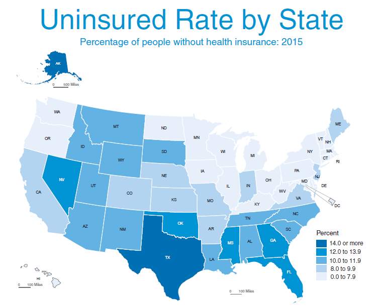
Demonstrated through heat map below are the rates for each state’s population without health insurance in 2015. Higher uninsured rates are presented with darker colors. Texas has a population of 4.6 million and has the highest uninsured rate in the country with 17.1%. Massachusetts has a population of 1.6 million and has the lowest rate of uninsured at 2.8%.

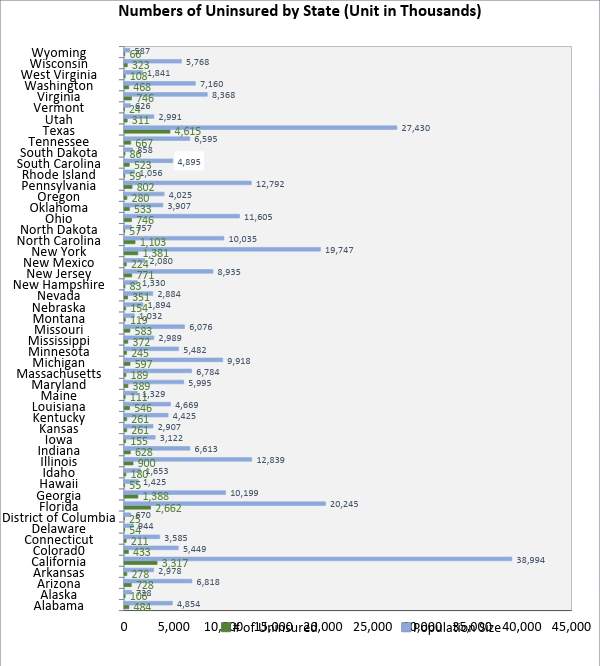
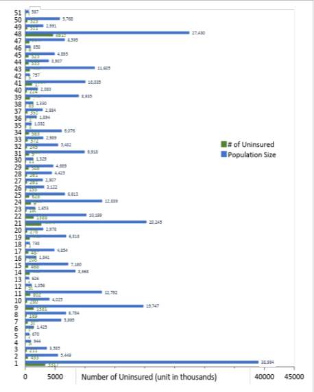
The chart below represents various individuals without insurance by the state in 2015 and each state’s population measure.  2015 rates for individuals without medical coverage for a full year schedule was 9.1 percent or close to 29 million aggregated from a populace of 321 million. In prospective from this data, we chose to examine which driving variables have an impact uninsured rate.

2. COLLECTION OF DATA

We attained and surveyed datasets from different hotspots for the uninsured rate for each of the 50 states along with choosing independent “predictors”. Discovery of distinctive datasets for unemployment rate, poverty, median income, age, Medicaid and Medicare, race/ethnicity, fertility rate for each of the 50 states combining the datasets with the end goal to play out through our investigation. Utilization of our datasets would span a period from 2014 to 2015. A final dataset was gathered through a blending of these datasets.

Datasets were sourced from the accompanying sources:

• Healthcare.gov – https://www.healthcare.gov/glossary/affordable-care-act
• Kaiser Family Foundation estimates based on the Census Bureau’s March 2016 Current Population Survey (CPS: Annual Social and Economic Supplement) – http://kff.org/
• United States Census Bureau – https://www.census.gov/data/datasets/2011/demo/ health-insurance/cps-revision.html
• U.S. Department of Health & Human Serves – https://aspe.hhs.gov/evaluations

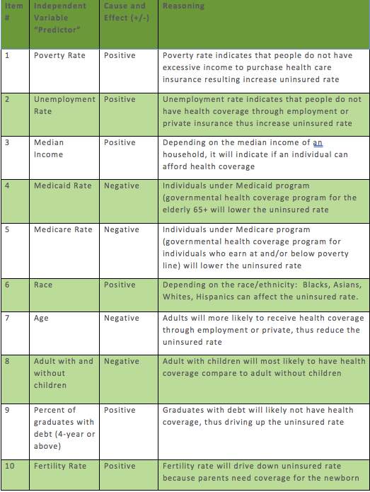
3. INDEPENDENT VARIABLES “PREDICTORS”

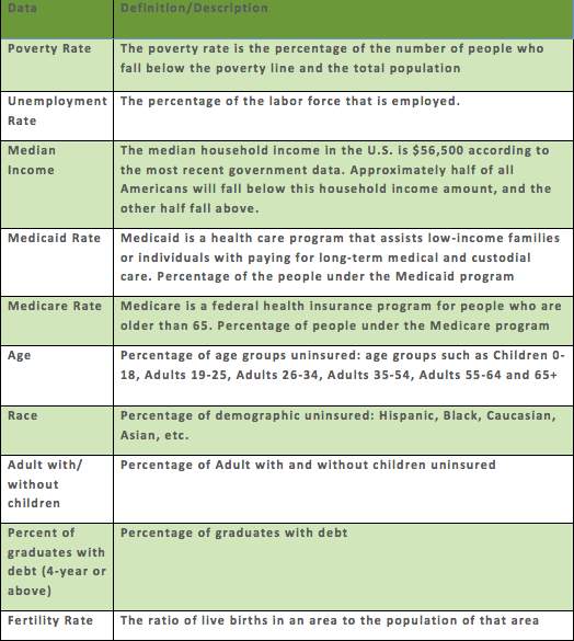
Analyzing the datasets and research has shown that there are multiple elements contributing to the uninsured rate, which is the dependent variable of interest in the regression analysis. As these stand, the decision was made to choose autonomous factors “indicators” that were decided to be the fundamental in driving clarity when describing the uninsured rate. Unified States Evaluation Agency defines independent variables and their related definitions contributing to uninsured rate characterized per the following:

4. DESCRIPTIVE ANALYSIS

Descriptive analysis is conducted to summarize the data set. Descriptive statistics are broken down further into measures of central tendency and measures of variability, or as spread.

4.1 Total U.S. States Statistics

Table1 below provides Descriptive Statistical information on each variable in the data set. On average, US states uninsured residents numbered around 8,721 in 2015 normalized per a population of 100,000 for the country. Massachusetts was the state with least uninsured rate and the highest uninsured rate belonged to Texas. As denoted by the table the mean and the median are almost equal which implies that the data is distributed evenly around the mean. Accordingly, having mean and median identical, provides insight that there are no outliers present.

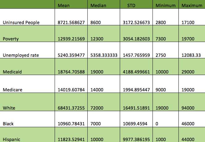
Table 1: Total US Statistics 

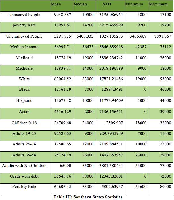
4.2 Southern States Statistics

Southern States Statistics show a minor difference in mean and median. Regardless of this only slight difference it has been interpreted to be almost same and concluded with the distribution of data also being symmetrical around the mean. Massachusetts carried the largest rate of uninsured citizens while the least number were located in District of Columbia. The lack of a difference in mean and mean suggests that there are no outlier values in the Southern State data.

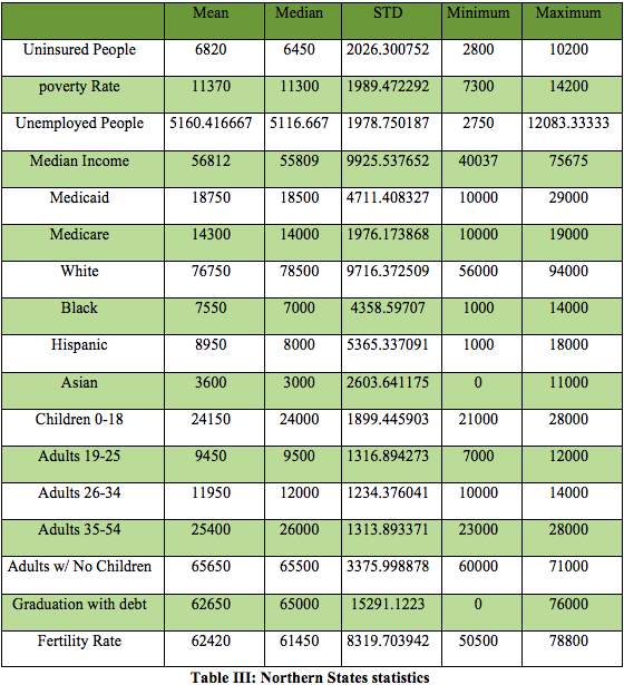
4.3 Northern States statistics

Northern States detailed the least uninsured rate or with the least number associated with Massachusetts and largest value in South Dakota. The mean and median are also same when compared at 100,000 people per sample which illustrates that the data is symmetrical distributed around the mean. This also evidences that here is shouldn’t be any outlier values in the Northern States.

5. REGRESSION ANALYSIS (REGRESSION)

5.1 Preliminary Assessments

Regression analysis was performed on the uninsured rate (dependent variable) and related independent “predictors” variables. This was conducted to determine how well the indicators could clarify the uninsured rate pertaining to each state. Ten independent variables were used to build the resulting multiple regression model. Prior to the regression model’s run, preparatory appraisals where performed on every independent variable’s cause and effect in relation to the dependent variable (uninsured rate). The independent variables appear to have a positive and  or negative impact on whether the uninsured rate will increase or decrease.

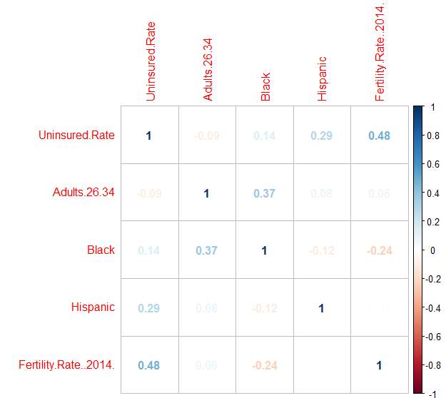
5.2 Correlation Matrix

A correlation matrix was run after concluding preliminary assessments for the independent variables to gain an overall view of multicollinearity between the dependent uninsured rate and independent variables

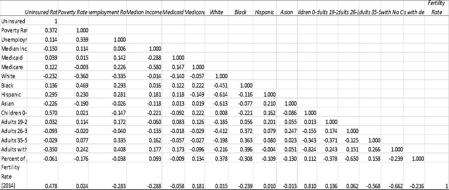
The table above shows that there are several variables which are highly correlated. To remove this multicollinearity VIF will be applied.

5.3 Variance inflation factor (VIF)

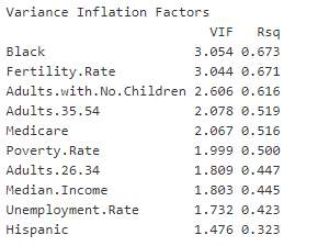
The Variance Inflation Factor (VIF) approach was used to identify and eliminate coefficients with high value of (VIF > 5). This measures the impact of collinearity among variables in question the amount of variance of the estimated regression coefficients is inflated being compared to the independent variables that are not linearly related.

Once the VIF regression was run, it was found that there were two coefficients with high VIF value that exceeded the threshold. These were White (22.78) and Children 0-18 (10.52), which were subsequently removed from the original dataset. Coefficients were then eliminated through VIF one by one and the regression model re-ran each time.   After completing the VIF, the P-value are checked.

5.4 P-value

Regression continued by checking P-values to test for remaining independent variable significances at a 5 percent level. The regression was run 10 times and variables were eliminated having a P-value greater than 0.05, consisting of adults 19-25 (0.97), Unemployment rate (0.61), Medicaid (0.67), Grads with Debts (0.66), Median Income (0.61), Adults with no children (0.46), Medicare (0.28), Asian (0.65), Adults 35-54 (0.23), Median Income (0.20). Regression analysis was run a last time resulting in the remaining Black, Hispanic, Adults 26-34, Fertility rate showing significance in terms of P-value.

The final regression output:

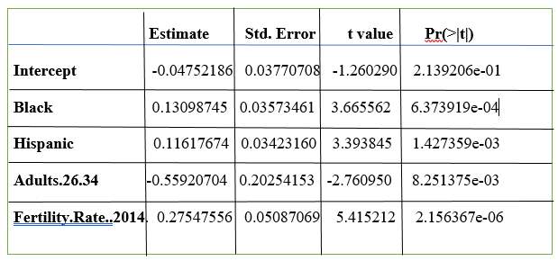
The final regression comprised four independent variables: Hispanic, Black, Adults 26-34 and Fertility Rate (2014).

Uninsured Rate = -0.0475 + 0.1309 *(Black) + 0.1161 *(Hispanic) + 0.2754 *(Fertility Rate) – 0.5592 *(Adults 26-23)

5.5 Multicollinearity Check of The Final Regression Variables

From the table, above it was discovered that there is no multi-collinearity, the variables are not closely related to each other.

5.6 Linear Regression

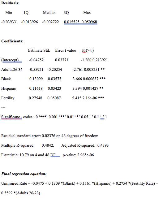
To see whether the variable from the final regression equation are significant a linear regression was then produced. From the result below show that all the 4 variables are highly significant.

Call:

Lm (formula = Uninsured Rate ~  [Adults 26-34] + Black + Hispanic + [Fertility Rate. 2014]  data = project2)

5.7 Interpretation

From the Final regression, the four main contributing factors in uninsured rate were Black, Hispanic, Adults 26-34 and Fertility Rate. Each factor was examined and interpreted in relation to its relationship/impact to the uninsured rate.

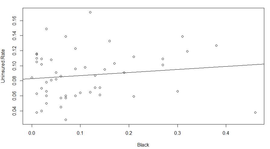
For each additional percentage increase of Black, uninsured rate is increased by 0.1309 percent on average in the state, with everything else held constant.

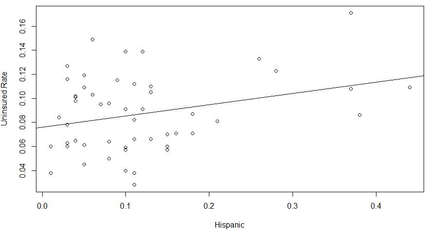
For each additional percentage increase of Hispanic, uninsured rate is increased by 0.1161 percent on average, with everything else held constant.

By isolating race component, it can be noted that there were discrepancies in uninsured rates between Asian Americans, Whites, Hispanic, Black and others. Within in the dataset, the Caucasian group had the lowest uninsured rate (9.1%) compared to Black (12.7%) and Hispanic (20.9%), which had the highest uninsured rate. The uninsured rate of Hispanics and Blacks were the highest contributing factor with disparities due to wealth between people of color and Caucasians.

A person of color who needs medical treatments is less likely to be able to afford medical insurance as a result of income disparities, this may be caused by educational level and citizenship status which drives social economic status. Blacks and Hispanics are probability earning lower to moderate-income and/or living within the federal poverty range. Some Hispanics could be recent migrants to the United States so and can only afford living expenses such as shelter and food with a higher uninsured rate. Blacks and Hispanics may also avoid taking out healthcare insurance because it is considered too expensive to obtain and getting treatments without insurance can put them into potential debt.

Hispanics and Blacks as contributing factors drove up uninsured rates in the states which was as concluded from the initial assessments.

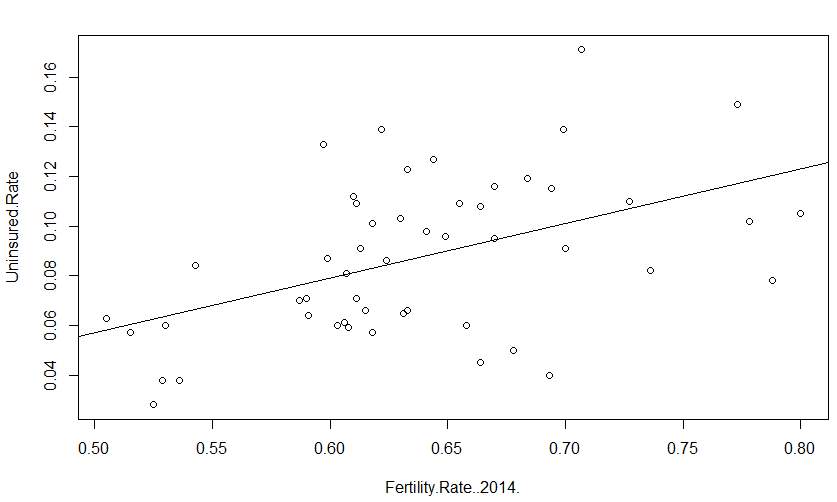
For every additional percentage of Fertility Rate, uninsured rate will be increased by 0.2754 percent on average in the state. While holding everything else constant.

Fertility Rate was a contributing factor driving up the uninsured rate. It could possibly be due to children were born into low-income families who cannot afford private insurance and/or lack access to supplemental government programs such as Children’s Health Insurance Program (CHIP) or Medicaid. Additionally, the child’s ethnicity might be another factor as to why they are uninsured. In 2014, the percentage of uninsured children by race showed Hispanic children being 9.6% uninsured whereas Caucasian were 4.9%. The result of Fertility as a contributor to uninsured rate was as expected and consistent with the assessment’s initial findings.

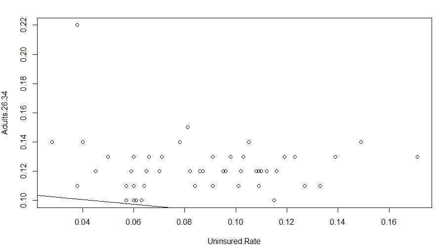
For every additional percentage of Adults 26-34, uninsured rate will be declined by .5592 percent on average in the state, with everything else held constant.

Adults 26-34 was a contributing factor in driving down uninsured rate could possibly due to employment. This group’s healthcare insurance could be covered by their employers thus allowing them to have greater access to treatments as needed. Adults 26-34 had a positive impact of uninsured rate as expected from the initial assessments of independent variables.

This final regression model had a coefficient of determination R² of 0.48. Thus, it was concluded that a 48 percent variation in the uninsured rate can be explained through variation in the four contributing factors: Hispanic, Black, Adults 26-34, and Fertility Rate.

6. RESIDUAL PLOT AND NORMALITY OF VARIANCE ANALYSIS

Validation of the regression model generated by this assessment met with the following four conditions: 1) Linearity, 2) Independence of Error, 3) Normality of Error, and 4) Equal Variance.

6.1 Residual plots

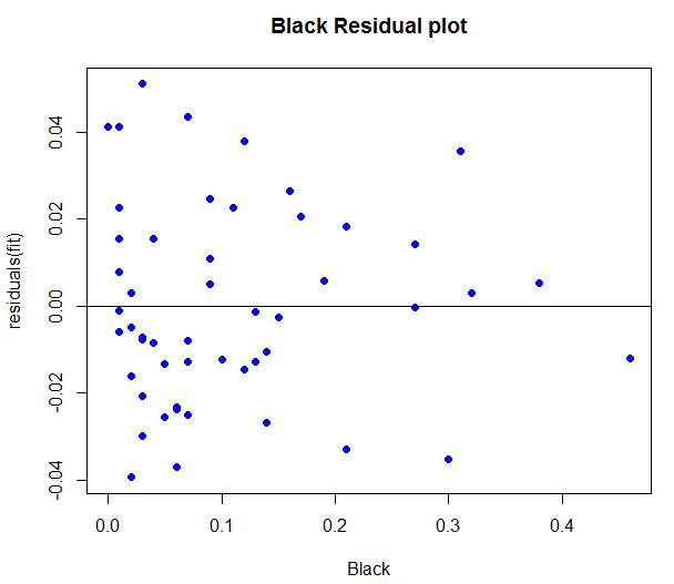
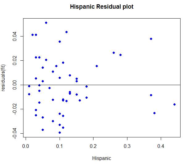
Residual plots were generated in R language for each independent variable from the final output and the patterns of each were observed.

The Black Residual Plot above shows each point on the plot appeared to have a random disbursement and shows no pattern of violating the heteroscedastic rule. It was then concluded that this model represents a good fit for the data set.

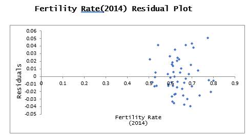
The Fertility Rate Residual Plot above shows each point on the plot appeared to disburse in a random manner and shows no pattern which violates the heteroscedastic rule. It was then concluded that this model was a great fit for the data set.

Reviewing the Hispanic Residual Plot above shows each point on the plot appeared to disburse randomly and showed no pattern of violating the heteroscedastic rule. It was then concluded that this model was a great fit for the data set.

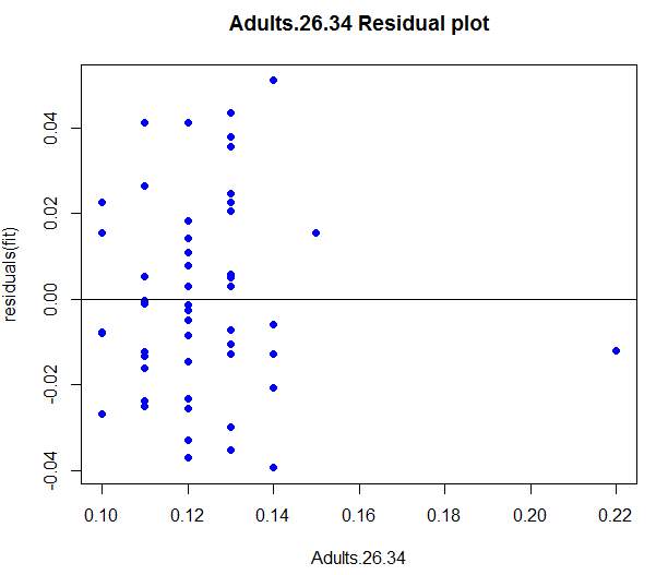
The Adult 26-34 residual plot shows it has one point value at 0.22 that appeared far from the cluster of data values. This point value was District of Columbia and showed that percentage of Adults 26-34 in District of Columbia had a high degree of difference compared to other states. However, the bulk of points on the plot appeared to disburse in a random manner and showing no pattern of violating the heteroscedastic rule. It was also concluded that this model was a great fit for the data set.

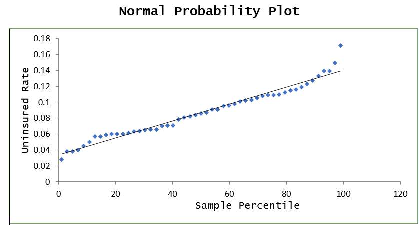
6.2 Normality

Checking for unusual and outlier points by reviewing the standardized residual values and found that value for Alaska was unusual at 2.27 as exhibited in the Normal Probably Plot below. However, it was inconsequential given that residuals/errors were almost perfectly linear. The conclusion was that the residuals or errors were normally distributed.

6.3 Histogram

A histogram produced of the standardized residuals shows that the data was normally distributed.

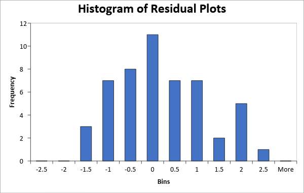
From review, it appeared that the residuals were normally distributed and there was no skewedness to the population data caused by outliners except for Alaska having the unusual value of 2.27, as the data exhibited bell-curved shape. The points on the Normal Probability Plot form a nearly linear pattern, indicating that the normal distribution was a good model for this data set. The data is normally distributed.

Based on the residual plots analysis and the normality of variance review, the uninsured rate regression model exhibits linearity, normality of error, independence of error and equal variance.

6.3.1 Conclusion

Based on the regression analysis performed, the four contributing factors to the uninsured rate in each state were Black, Hispanic, Adults 26-34 and Fertility Rate. Blacks and Hispanics raised the country’s uninsured rate and Adults between 26-34 age group decreased the country’s uninsured rates. Wealth disparities among ethnicity groups could be a cause and Adults 26-34 age group are more likely to be employed and have health care provided by employers.

7. HYPOTHESIS TESTING

Along with discovering and examining the contributing factors to the uninsured rate in the US, a closer look was taken into whether states which dominated by Republican or Democratic had higher numbers of uninsured in 2015 as an early assessment.   Four main factors which impacted uninsured rate to determine whether these factors were predominate in both Republican or Democratic states. The below graph illustrates the uninsured population in the Republican’s states versus Democratic states in 2015:

In 2015, there were 29.7 million or 9% (of total population size of 320.8 million) of uninsured individuals in the states. 28% (8.5 million) of the 29.7 million uninsured were population from Democratic states and 71% (21.2 million) were Republican states. Relating to the total population size of 320.8 million in the U.S., Democratic values comprised 3% and Republican comprised of 7%. It was evident to conclude that Democratic states had a lower portion of individuals uninsured compared to Republican’s states.

Four one-tail tests were used on the four contributing factors from the final regression model based on Black, Hispanic, Adults 26-34 and Fertility Rate to determine whether these factors were predominating in the Democratic states or Republican’s states.

1) One-tailed Test assuming equal variances for % of Blacks between the Republican and Democratic States

A one tail t – Test assuming equal variances to determine if the mean difference in percentage of Blacks in the Democratic States ≥ in the percentage of Blacks in the Republican States.

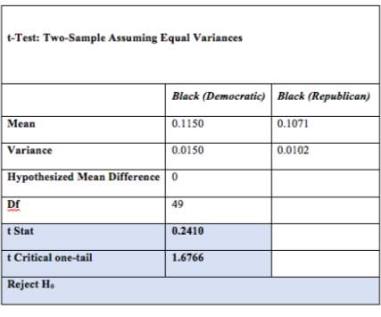
The test resulted in the tstat < Tcritical. This means that the tstat rests in the rejection region. It was then rejected for the null hypotheses H0 and concluded that the mean difference in percentage of Blacks in the Democratic states was less than the percentage of Blacks in the Republican’s states. There were less uninsured for the Black group in the states dominated by Democratic affiliation versus Republican.

2) One-tailed Test assuming equal variances for % of Hispanic between the Republican and Democratic States

A one tail t – Test was conducted assuming equal variances to determine if the mean difference in percentage of Hispanic in the Democratic states ≥ the percentage of Hispanic in the Republican’s states.

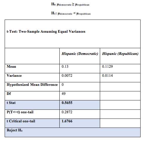
The results found that the tstat < Tcritical. This means that the tstat lies in the rejection region. The null hypotheses H0 was rejected and concluded that the mean difference in percentage of Hispanic in the Democratic states was less than the mean difference in the percentage of Hispanics in the Republican’s states. Uninsured rate for the Hispanic group in states dominated by Democratic was less compared to Republican.

3) One-tailed Test assuming equal variances for % of Fertility Rate (2014) between the Republican and Democratic States

The one tail t – Test assuming equal variances in determining whether the mean difference in percentage of Fertility Rate (2014) in the Republican States ≥ percentage of Fertility Rate (2014) in the Democratic States.

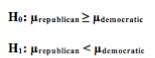
After performing the test, it was found that the tstat > Tcritical. This means that the tstat does not lie in the rejection region.  Failing to reject the null hypotheses H0 concluded that the mean difference in percentage of Fertility Rate (2004) in the Republican States was greater than or equal to percentage of Fertility Rate (2004) in the Democratic States. Based on the result, Republican’s states possessed a higher fertility rate relative to Democratic States.

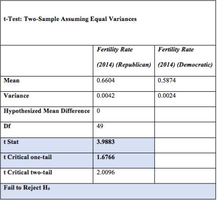
4) One-tailed Test assuming equal variances for % of Adults (26-34) between the Republican and Democratic States Performing a one tail t – Test assuming equal variances to determine if the mean difference in Percentage of Adults (26-34) in the Republican’s tates ≥ percentage of Adults (26-34) in the Democratic states.

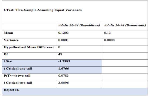
After performing the test, it was found that the tstat < Tcritical, meaning that the tstat lies in the rejection region. The null hypotheses H0 was rejected and concluded that the mean difference in percentage of Adults (26-34) in the Republican States was less than percentage of Adults (26-34) in the Democratic States. From this result, it can be concluded that there were more working adults in the Democratic states compared with Republican’s states (elderly/retired work group).

8. OVERALL CONCLUSION

Based on the analysis on uninsured rate for the states, the four contributing factors to uninsured rate with the most impact were Black, Hispanic, Fertility Rate and Adults 26-34. 48%. Variation for uninsured rate may be explained by the factors observed though each method of testing.  Republican’s states had the highest contribution of uninsured individuals (21.2 million or 71% of uninsured) or at a rate 7%.

9. FINAL NOTES

Affordable Health Care Act is essential for the American population residing within its borders. Should the current Administration successfully repeal and implement a new healthcare plan, the negative outcomes might have a potential catastrophic effect. Those impacted by this situation the most are children, elderly 65+, veterans, and people existing at the poverty level who could be rejected from their current coverage plan.  It would be beneficial for the current Administration to review and evaluate the demographic data in each state to assist in implementing adequate healthcare for its citizens.

9.1 References

Kaiser Family Foundation estimates based on the Census Bureau’s March 2016 Current Population Survey (CPS: Annual Social and Economic Supplement) –  http://kff.org/

U.S. Department of Health & Human Serves – https://aspe.hhs.gov/evaluations

United States Census Bureau – https://www.census.gov/data/datasets/2011/demo/health-insurance/cps-revision.html

Healthcare.gov – https://www.healthcare.gov/glossary/affordable-care-act

10. APPENDIX (R) EQUATIONS

> project<-read.csv(“project dataset.csv”)

> summary(project)

Uninsured.Rate     Poverty.Rate    Unemployment.Rate Median.Income      Medicaid     Medicare          White            Black           Hispanic

Min.   :0.02800   Min. :0.0730   Min. :0.02750 Min.   :40037 Min. :0.1000 Min.   :0.0900 Min. :0.1900 Min. :0.0000   Min. :0.0100

1st Qu.:0.06200   1st Qu.:0.1080 1st Qu.:0.04254   1st Qu.:50783 1st Qu.:0.1700 1st Qu.:0.1300   1st Qu.:0.5800 1st Qu.:0.0300 1st Qu.:0.0500

Median :0.08600   Median :0.1230 Median :0.05358   Median :56473 Median :0.1900 Median :0.1400   Median :0.7200 Median :0.0700 Median :0.1000

Mean   :0.08722   Mean :0.1294   Mean :0.05240 Mean   :56925 Mean :0.1876 Mean   :0.1402 Mean :0.6843 Mean :0.1096   Mean :0.1182

3rd Qu.:0.10900   3rd Qu.:0.1460 3rd Qu.:0.05971   3rd Qu.:62561 3rd Qu.:0.2150 3rd Qu.:0.1500   3rd Qu.:0.8050 3rd Qu.:0.1450 3rd Qu.:0.1400

Max.   :0.17100   Max. :0.1970   Max. :0.12083 Max.   :75675 Max. :0.2900 Max.   :0.1900 Max. :0.9400 Max. :0.4600   Max. :0.4400

Asian         Children.0.18    Adults.19.25     Adults.26.34     Adults.35.54    Adults.with.No.Children Percent.of.graduates.with.debt..4.year.or.above.

Min.   :0.00000   Min. :0.1800   Min. :0.07000 Min.   :0.1000 Min. :0.2300  Min. :0.5300     Min.   :0.0000

1st Qu.:0.02000   1st Qu.:0.2300 1st Qu.:0.09000   1st Qu.:0.1100 1st Qu.:0.2500 1st Qu.:0.6300          1st Qu.:0.5500

Median :0.03000   Median :0.2400 Median :0.09000   Median :0.1200 Median :0.2600 Median :0.6500          Median :0.6100

Mean   :0.04157   Mean :0.2449   Mean :0.09333 Mean   :0.1233 Mean :0.2563  Mean :0.6525     Mean   :0.5839

3rd Qu.:0.05000   3rd Qu.:0.2600 3rd Qu.:0.10000   3rd Qu.:0.1300 3rd Qu.:0.2650 3rd Qu.:0.6700          3rd Qu.:0.6600

Max.   :0.39000   Max. :0.3200   Max. :0.12000 Max.   :0.2200 Max. :0.2900  Max. :0.7700     Max.   :0.7600

Fertility.Rate..2014.

Min.   :0.5050

1st Qu.:0.6045

Median :0.6300

Mean   :0.6375

3rd Qu.:0.6740

Max.   :0.8000

> model1<-lm(Uninsured.Rate~.,data=project)

> library(car)

> vif(model1)

Poverty.Rate           Unemployment.Rate                                   Median.Income

2.347919            2.080824                                         2.309152

Medicaid            Medicare                                           White

1.467078            2.472166                                        22.784637

Black      Hispanic                                           Asian

10.524648              8.745064                                       8.161150

Children.0.18                  Adults.19.25                                   Adults.26.34

10.539536              1.892653                                       2.927854

Adults.35.54     Adults.with.No.Children Percent.of.graduates.with.debt..4.year.or.above.

2.752132            6.664773                                         3.240549

Fertility.Rate..2014.

7.752917

> model2=lm(Uninsured.Rate~ Poverty.Rate+Unemployment.Rate+Median.Income+Medicaid+Medicare+Black+Hispanic+Asian+Children.0.18+Adults.19.25+Adults.26.34+Adults.35.54+    Adults.with.No.Children+Percent.of.graduates.with.debt..4.year.or.above.+Fertility.Rate..2014.,data=project)

> vif(model2)

Poverty.Rate           Unemployment.Rate                                   Median.Income

2.257864            1.970529                                         2.308730

Medicaid            Medicare                                           Black

1.466953            2.462321                                         4.278976

Hispanic               Asian                              Children.0.18

2.339912            1.257848                                        10.525540

Adults.19.25                Adults.26.34                                     Adults.35.54

1.846740            2.926635                                         2.751158

Adults.with.No.Children Percent.of.graduates.with.debt..4.year.or.above.                            Fertility.Rate..2014.

6.644467            3.210439                                         7.119587

> model3=lm(Uninsured.Rate~ Poverty.Rate+Unemployment.Rate+Median.Income+Medicaid+Medicare+Black+Hispanic+Asian+Adults.19.25+Adults.26.34+Adults.35.54+    Adults.with.No.Children+Percent.of.graduates.with.debt..4.year.or.above.+Fertility.Rate..2014.,data=project)

> vif(model3)

Poverty.Rate           Unemployment.Rate                                   Median.Income

2.224262            1.765450                                         2.229527

Medicaid            Medicare                                           Black

1.417419            2.418827                                         3.525274

Hispanic               Asian                               Adults.19.25

1.922345            1.244239                                         1.793971

Adults.26.34                Adults.35.54                          Adults.with.No.Children

2.710687            2.718416                                         3.624344

Percent.of.graduates.with.debt..4.year.or.above.                            Fertility.Rate..2014.

2.961608            4.036953

> summary(model3)$coef

Estimate Std. Error     t value   Pr(>|t|)

(Intercept)                                       1.691038e-02 2.508029e-01 0.06742500 0.94661646

Poverty.Rate                                      8.015433e-02 1.662638e-01 0.48209115 0.63265938

Unemployment.Rate                                 1.597270e-01 3.103414e-01 0.51468145 0.60992130

Median.Income                                    -8.913001e-07 5.533781e-07 -1.61065310 0.11599005

Medicaid                                         -4.100594e-02 9.678108e-02 -0.42369787 0.67430709

Medicare                                         -3.023145e-01 2.654496e-01 -1.13887731 0.26227634

Black                                             1.188335e-01 5.974952e-02 1.98886115 0.05435826

Hispanic                                          1.219541e-01 4.731498e-02 2.57749430 0.01419357

Asian                                            -1.174639e-01 6.578126e-02 -1.78567399 0.08257871

Adults.19.25                                     -1.078209e-02 4.186424e-01 -0.02575489 0.97959508

Adults.26.34                                     -3.553223e-01 3.064314e-01 -1.15954938 0.25386551

Adults.35.54                                      2.568028e-01 4.096002e-01 0.62695978 0.53464181

Adults.with.No.Children                          -1.010383e-01 1.765919e-01 -0.57215747 0.57077123

Percent.of.graduates.with.debt..4.year.or.above.  1.876918e-02 4.226524e-02 0.44408072 0.65964225

Fertility.Rate..2014.                             2.569567e-01 9.908688e-02 2.59324665 0.01365907

> model4=lm(Uninsured.Rate~ Poverty.Rate+Unemployment.Rate+Median.Income+Medicaid+Medicare+Black+Hispanic+Asian+Adults.26.34+Adults.35.54+    Adults.with.No.Children+Percent.of.graduates.with.debt..4.year.or.above.+Fertility.Rate..2014.,data=project)

> summary(model4)$coef

Estimate Std. Error     t value   Pr(>|t|)

(Intercept)                                       1.526618e-02 2.392438e-01 0.06381012 0.94946492

Poverty.Rate                                      8.079750e-02 1.621427e-01 0.49831108 0.62121414

Unemployment.Rate                                 1.589390e-01 3.046304e-01 0.52174363 0.60495834

Median.Income                                    -8.915180e-07 5.457900e-07 -1.63344498 0.11085756

Medicaid                                         -4.073642e-02 9.490543e-02 -0.42923169 0.67024375

Medicare                                         -3.034121e-01 2.584438e-01 -1.17399664 0.24789783

Black                                             1.186604e-01 5.856321e-02 2.02619411 0.04999982

Hispanic                                          1.216091e-01 4.476259e-02 2.71675839 0.00996619

Asian                                            -1.174339e-01 6.487667e-02 -1.81010988 0.07840671

Adults.26.34                                     -3.538260e-01 2.967823e-01 -1.19220736 0.24077040

Adults.35.54                                      2.612511e-01 3.663544e-01 0.71311033 0.48025123

Adults.with.No.Children                          -1.020900e-01 1.694702e-01 -0.60240676 0.55057777

Percent.of.graduates.with.debt..4.year.or.above.  1.905461e-02 4.023181e-02 0.47362036 0.63855341

Fertility.Rate..2014.                             2.569022e-01 9.771725e-02 2.62903589 0.01239824

> model5=lm(Uninsured.Rate~ Poverty.Rate+Unemployment.Rate+Median.Income+Medicare+Black+Hispanic+Asian+Adults.26.34+Adults.35.54+    Adults.with.No.Children+Percent.of.graduates.with.debt..4.year.or.above.+Fertility.Rate..2014.,data=project)

> summary(model5)$coef

Estimate Std. Error     t value    Pr(>|t|)

(Intercept)                                      -3.241112e-03 2.327868e-01 -0.01392309 0.988964181

Poverty.Rate                                      9.747379e-02 1.557204e-01 0.62595404 0.535087046

Unemployment.Rate                                 1.554375e-01 3.012348e-01 0.51600117 0.608843215

Median.Income                                    -7.963881e-07 4.933835e-07 -1.61413610 0.114772428

Medicare                                         -2.838773e-01 2.516595e-01 -1.12802139 0.266382837

Black                                             1.106334e-01 5.489818e-02 2.01524782 0.050992438

Hispanic                                          1.152908e-01 4.181683e-02 2.75704356 0.008913333

Asian                                            -1.158124e-01 6.406764e-02 -1.80765854 0.078580583

Adults.26.34                                     -3.264313e-01 2.867106e-01 -1.13853926 0.262022542

Adults.35.54                                      2.974589e-01 3.526632e-01 0.84346443 0.404247113

Adults.with.No.Children                          -1.154655e-01 1.647829e-01 -0.70071276 0.487750957

Percent.of.graduates.with.debt..4.year.or.above.  1.734897e-02 3.960304e-02 0.43807160 0.663814615

Fertility.Rate..2014.                             2.558994e-01 9.663506e-02 2.64810105 0.011721698

> model6=lm(Uninsured.Rate~ Poverty.Rate+Unemployment.Rate+Median.Income+Medicare+Black+Hispanic+Asian+Adults.26.34+Adults.35.54+    Adults.with.No.Children+Fertility.Rate..2014.,data=project)

> summary(model6)$coef

Estimate Std. Error    t value    Pr(>|t|)

(Intercept)              4.556156e-02 2.022703e-01  0.2252508 0.822960333

Poverty.Rate             9.959200e-02 1.540243e-01  0.6465992 0.521678773

Unemployment.Rate        1.524032e-01 2.980188e-01  0.5113877 0.611962905

Median.Income           -7.627245e-07 4.822868e-07 -1.5814749 0.121846624

Medicare                -2.503324e-01 2.372302e-01 -1.0552301 0.297813548

Black                    1.076432e-01 5.390486e-02  1.9969099 0.052847592

Hispanic                 1.137249e-01 4.122987e-02  2.7583138 0.008798634

Asian                   -1.148315e-01 6.336168e-02 -1.8123184 0.077641078

Adults.26.34            -3.887347e-01 2.463570e-01 -1.5779324 0.122658995

Adults.35.54             2.857040e-01 3.479788e-01  0.8210387 0.416614946

Adults.with.No.Children -1.475551e-01 1.460688e-01 -1.0101751 0.318637961

Fertility.Rate..2014.    2.350399e-01 8.321345e-02  2.8245424 0.007423150

> model7=lm(Uninsured.Rate~ Poverty.Rate+Median.Income+Medicare+Black+Hispanic+Asian+Adults.26.34+Adults.35.54+    Adults.with.No.Children+Fertility.Rate..2014.,data=project)

>   summary(model7)$coef

Estimate Std. Error    t value    Pr(>|t|)

(Intercept)              2.104046e-02 1.946823e-01  0.1080759 0.914475780

Poverty.Rate             1.115169e-01 1.508369e-01  0.7393210 0.464028888

Median.Income           -7.598992e-07 4.777827e-07 -1.5904703 0.119602375

Medicare                -2.144541e-01 2.245168e-01 -0.9551809 0.345223559

Black                    1.067682e-01 5.337804e-02  2.0002276 0.052296766

Hispanic                 1.201001e-01 3.893552e-02  3.0845903 0.003687803

Asian                   -1.177666e-01 6.251599e-02 -1.8837840 0.066877903

Adults.26.34            -3.942582e-01 2.438376e-01 -1.6168887 0.113762771

Adults.35.54             3.238559e-01 3.367352e-01  0.9617526 0.341952042

Adults.with.No.Children -1.240169e-01 1.373416e-01 -0.9029810 0.371941850

Fertility.Rate..2014.    2.362664e-01 8.240748e-02  2.8670512 0.006579346

>

> model8=lm(Uninsured.Rate~ Median.Income+Medicare+Black+Hispanic+Asian+Adults.26.34+Adults.35.54+    Adults.with.No.Children+Fertility.Rate..2014.,data=project)

> summary(model8)$coef

Estimate Std. Error    t value     Pr(>|t|)

(Intercept)              2.682289e-02 1.934465e-01  0.1386579 0.8903993010

Median.Income           -7.856594e-07 4.738684e-07 -1.6579695 0.1049565708

Medicare                -2.467908e-01 2.189942e-01 -1.1269284 0.2663252544

Black                    1.288895e-01 4.395838e-02  2.9320800 0.0054864593

Hispanic                 1.323881e-01 3.501459e-02  3.7809399 0.0004991096

Asian                   -1.256407e-01 6.126054e-02 -2.0509230 0.0467019733

Adults.26.34            -4.625731e-01 2.244003e-01 -2.0613745 0.0456465398

Adults.35.54             2.928552e-01 3.322617e-01  0.8813991 0.3832398437

Adults.with.No.Children -9.810179e-02 1.320569e-01 -0.7428751 0.4617927887

Fertility.Rate..2014.    2.528251e-01 7.886576e-02  3.2057652 0.0026106740

>

>model9=lm(Uninsured.Rate~ Median.Income+Medicare+Black+Hispanic+Asian+Adults.26.34+Adults.35.54+Fertility.Rate..2014.,data=project)

>summary(model9)$coef

Estimate Std. Error    t value     Pr(>|t|)

(Intercept)           -8.039946e-02 1.281099e-01 -0.6275819 5.336753e-01

Median.Income         -7.744079e-07 4.710928e-07 -1.6438543 1.076724e-01

Medicare              -2.367738e-01 2.174094e-01 -1.0890685 2.823333e-01

Black                  1.174780e-01 4.096671e-02  2.8676456 6.441194e-03

Hispanic               1.306089e-01 3.474572e-02  3.7589913 5.208723e-04

Asian                 -1.292730e-01 6.073844e-02 -2.1283560 3.921792e-02

Adults.26.34          -4.649308e-01 2.231776e-01 -2.0832319 4.335492e-02

Adults.35.54           3.653614e-01 3.159040e-01  1.1565583 2.539891e-01

Fertility.Rate..2014.  2.912300e-01 5.923952e-02  4.9161430 1.397068e-05

>model10=lm(Uninsured.Rate~ Median.Income+Black+Hispanic+Asian+Adults.26.34+Adults.35.54+Fertility.Rate..2014.,data=project)

>summary(model10)$coef

Estimate Std. Error t value     Pr(>|t|)

(Intercept)           -1.384950e-01 1.167273e-01 -1.186484 2.419456e-01

Median.Income         -4.731843e-07 3.821736e-07 -1.238140 2.223817e-01

Black                  1.006674e-01 3.802944e-02  2.647090 1.130083e-02

Hispanic               1.297808e-01 3.481248e-02  3.727996 5.593514e-04

Asian                 -1.330086e-01 6.077257e-02 -2.188629 3.410260e-02

Adults.26.34          -3.939066e-01 2.138979e-01 -1.841563 7.244357e-02

Adults.35.54           3.847631e-01 3.160829e-01  1.217285 2.301343e-01

Fertility.Rate..2014.  2.851399e-01 5.910246e-02  4.824501 1.794712e-05

>model11=lm(Uninsured.Rate~ Median.Income+Black+Hispanic+Asian+Adults.26.34+Fertility.Rate..2014.,data=project)

>summary(model11)$coef

Estimate Std. Error    t value     Pr(>|t|)

(Intercept)           -9.490777e-03 4.919700e-02 -0.1929137 8.479142e-01

Median.Income         -4.915828e-07 3.839596e-07 -1.2802983 2.071489e-01

Black                  1.190585e-01 3.509008e-02  3.3929386 1.472464e-03

Hispanic               1.371117e-01 3.447482e-02  3.9771550 2.564702e-04

Asian                 -1.257977e-01 6.081341e-02 -2.0685851 4.449253e-02

Adults.26.34          -4.715547e-01 2.052799e-01 -2.2971306 2.642732e-02

Fertility.Rate..2014.  2.491273e-01 5.144447e-02  4.8426450 1.618423e-05

> model12=lm(Uninsured.Rate~ Black+Hispanic+Asian+Adults.26.34+Fertility.Rate..2014.,data=project)

> summary(model12)$coef

Estimate Std. Error t value     Pr(>|t|)

(Intercept)           -0.0517178 0.03676204 -1.406826 1.663481e-01

Black                  0.1191127 0.03533838 3.370632 1.548089e-03

Hispanic               0.1270623 0.03380693 3.758470 4.901400e-04

Asian                 -0.1145422 0.06060045 -1.890121 6.519286e-02

Adults.26.34          -0.4470993 0.20583568 -2.172118 3.515497e-02

Fertility.Rate..2014.  0.2678601 0.04966892 5.392911 2.461450e-06

>

> model13=lm(Uninsured.Rate~ Black+Hispanic+Adults.26.34+Fertility.Rate..2014.,data=project)

> summary(model13)$coef

Estimate Std. Error t value     Pr(>|t|)

(Intercept)           -0.04752186 0.03770708 -1.260290 2.139206e-01

Black                  0.13098745 0.03573461 3.665562 6.373919e-04

Hispanic               0.11617674 0.03423160 3.393845 1.427359e-03

Adults.26.34          -0.55920704 0.20254153 -2.760950 8.251375e-03

Fertility.Rate..2014.  0.27547556 0.05087069 5.415212 2.156367e-06

Finall regression equation:

-0.048 -0.559(Adults 26-34) + 0.131(black) + 0.116(hispanic) + 0.275(fertility rate)

> cor(project)

Uninsured.Rate Poverty.Rate Unemployment.Rate Median.Income     Medicaid    Medicare        White       Black

Uninsured.Rate                                       1.00000000 0.37202604     0.113874175  -0.150363513 0.038769683  0.12222877 -0.232483572 0.13607174

Poverty.Rate                                         0.37202604 1.00000000     0.338980133   0.114205665 0.015119221 -0.00275479 -0.360332259  0.46898588

Unemployment.Rate                                    0.11387418 0.33898013     1.000000000   0.005773403 0.142134610  0.22615967 -0.334539615 0.29270743

Median.Income                                       -0.15036351 0.11420567     0.005773403   1.000000000 -0.287829343 -0.57970862 -0.013959282  0.01567754

Medicaid                                             0.03876968 0.01511922     0.142134610  -0.287829343 1.000000000  0.14657273 -0.139507918 0.12162506

Medicare                                             0.12222877 -0.00275479     0.226159666  -0.579708621 0.146572731  1.00000000 -0.056799162 0.22211006

White                                               -0.23248357 -0.36033226     -0.334539615  -0.013959282 -0.139507918 -0.05679916  1.000000000 -0.45147403

Black                                                0.13607174 0.46898588     0.292707427   0.015677536 0.121625056  0.22211006 -0.451474032 1.00000000

Hispanic                                             0.29487656 0.23027317     0.281380831   0.181095026 0.118153006 -0.14853768 -0.614324594 -0.11622250

Asian                                               -0.22642605 -0.19010563     -0.025896107  -0.117926559 0.013135202  0.01882848 -0.613436578 -0.07695249

Children.0.18                                        0.57022928 0.02127614     -0.147346458  -0.220964812 -0.092248811  0.22174941 0.008080492 -0.22102449

Adults.19.25                                         0.03202191 0.11441566     0.172193574  -0.059558174 0.083283840  0.12577899 -0.185175812 0.05605426

Adults.26.34                                        -0.09258322 -0.01992618     -0.040018497  -0.135157890 -0.018271042 -0.02922822 -0.411896179  0.37159121

Adults.35.54                                        -0.02939282 0.07666192     0.334510515   0.161800781 -0.057382961 -0.02653467 -0.198033820  0.36313500

Adults.with.No.Children                             -0.35049526 0.24189085     0.408401507   0.176632710 0.173089747 -0.09629096 -0.215944798  0.39644998

Percent.of.graduates.with.debt..4.year.or.above.    -0.06085586 -0.17570309     -0.037579130   0.092790768 -0.008711858  0.13422269 0.378278976 -0.30757730

Fertility.Rate..2014.                                0.47781711 0.02390335     -0.282747411  -0.287999139 -0.058103343  0.18129729 0.014741186 -0.23920220

Hispanic     Asian Children.0.18 Adults.19.25 Adults.26.34 Adults.35.54 Adults.with.No.Children

Uninsured.Rate                                    0.294876564 -0.22642605 0.570229280 0.03202191  -0.09258322 -0.02939282     -0.350495258

Poverty.Rate                                      0.230273168 -0.19010563 0.021276142 0.11441566  -0.01992618 0.07666192     0.241890849

Unemployment.Rate                                 0.281380831 -0.02589611 -0.147346458 0.17219357  -0.04001850 0.33451051     0.408401507

Median.Income                                     0.181095026 -0.11792656 -0.220964812 -0.05955817  -0.13515789 0.16180078     0.176632710

Medicaid                                          0.118153006 0.01313520 -0.092248811 0.08328384  -0.01827104 -0.05738296     0.173089747

Medicare                                         -0.148537682 0.01882848 0.221749406 0.12577899  -0.02922822 -0.02653467     -0.096290961

White                                            -0.614324594 -0.61343658 0.008080492 -0.18517581  -0.41189618 -0.19803382     -0.215944798

Black                                            -0.116222503 -0.07695249 -0.221024486 0.05605426   0.37159121 0.36313500     0.396449979

Hispanic                                          1.000000000 0.21019117 0.161874620 0.20057432   0.07889318 0.07992494     -0.003662059

Asian                                             0.210191175 1.00000000 -0.086344403 0.05511859   0.24679120 0.02269750     0.050923097

Children.0.18                                     0.161874620 -0.08634440 1.000000000 0.01339958  -0.15479295 -0.34306193     -0.824044927

Adults.19.25                                      0.200574325 0.05511859 0.013399584 1.00000000   0.17395683 -0.37061654     0.243418386

Adults.26.34                                      0.078893183 0.24679120 -0.154792948 0.17395683   1.00000000 -0.12496912     0.150904521

Adults.35.54                                      0.079924944 0.02269750 -0.343061927 -0.37061654  -0.12496912 1.00000000     0.265732888

Adults.with.No.Children                          -0.003662059 0.05092310 -0.824044927 0.24341839   0.15090452 0.26573289     1.000000000

Percent.of.graduates.with.debt..4.year.or.above. -0.108798399 -0.13021238   0.111938837 -0.37830750 -0.65031230 0.15836059     -0.238989882

Fertility.Rate..2014.                             0.010493129 -0.01274000 0.810169716 0.13579777   0.06154469 -0.56764538     -0.662071859

Percent.of.graduates.with.debt..4.year.or.above. Fertility.Rate..2014.

Uninsured.Rate                                                                       -0.060855861     0.47781711

Poverty.Rate                                                                         -0.175703085     0.02390335

Unemployment.Rate                                                                    -0.037579130     -0.28274741

Median.Income                                                                         0.092790768     -0.28799914

Medicaid                                                                             -0.008711858     -0.05810334

Medicare                                                                              0.134222692     0.18129729

White                                                                                 0.378278976     0.01474119

Black                                                                                -0.307577295     -0.23920220

Hispanic                                                                             -0.108798399     0.01049313

Asian                                                                                -0.130212384     -0.01274000

Children.0.18                                                                         0.111938837     0.81016972

Adults.19.25                                                                         -0.378307503     0.13579777

Adults.26.34                                                                         -0.650312304     0.06154469

Adults.35.54                                                                          0.158360591     -0.56764538

Adults.with.No.Children                                                              -0.238989882     -0.66207186

Percent.of.graduates.with.debt..4.year.or.above.                                      1.000000000     -0.21558897

Fertility.Rate..2014.                                                                -0.215588966     1.00000000

CORRELATION

> library(corrplot)

> M <- cor(project2)

> corrplot(M, method=”number”)

REGREAAION:

> regression<-read.csv(“project2.csv”,header=TRUE)

>

> attach regression

Error: unexpected symbol in “attach regression”

> attach(regression)

> names(regression)

[1] “Uninsured.Rate”        “Adults.26.34”     “Black”

[4] “Hispanic”              “Fertility.Rate..2014.”

> plot(Uninsured.Rate,Adults.26.34)

> abline(lm(Uninsured.Rate~Adults.26.34))

> plot(Uninsured.Rate~Black)

> abline(lm(Uninsured.Rate~Black))

> plot(Uninsured.Rate~Hispanic)

> abline(lm(Uninsured.Rate~Hispanic))

> plot(Uninsured.Rate~Fertility.Rate..2014.)

> abline(lm(Uninsured.Rate~Fertility.Rate..2014.))

> results=lm(Uninsured.Rate~Adults.26. 34+Black+Hispanic+Fertility.Rate..2014.,data=project2)

> results

Call:

lm(formula = Uninsured. Rate ~ Adults.26.34 + Black + Hispanic +

Fertility.Rate..2014., data = project2)

Coefficients:

(Intercept)       Adults.26.34               Black

-0.04752             -0.55921               0.13099

Hispanic       Fertility.Rate.2014.

0.11618            0.27548

> summary(results)

Call:

lm(formula = Uninsured.Rate ~ Adults.26.34 + Black + Hispanic +

Fertility.Rate..2014., data = project2)

Residuals:

Min       1Q     Median        3Q     Max

-0.039331   -0.013926    -0.002722   0.015525 0.050968

Coefficients:

Estimate Std. Error t value Pr(>|t|)

(Intercept)           -0.04752    0.03771  -1.260 0.213921

Adults.26.34          -0.55921    0.20254  -2.761 0.008251 **

Black                  0.13099    0.03573   3.666 0.000637 ***

Hispanic               0.11618    0.03423   3.394 0.001427 **

Fertility.Rate.2014.  0.27548    0.05087    5.415 2.16e-06 ***

—

Signif. codes:  0 ‘***’ 0.001 ‘**’ 0.01 ‘*’ 0.05 ‘.’ 0.1 ‘ ’ 1

Residual standard error: 0.02376 on 46 degrees of freedom

Multiple R-squared:  0.4842,    Adjusted R-squared:  0.4393

F-statistic: 10.79 on 4 and 46 DF,  p-value: 2.965e-06

> fit=lm(Uninsured.Rate~ Black+Hispanic+Adults.26.34+Fertility.Rate..2014.,data=project2)

> setwd(“C:/Users/user/Desktop”)

> states=read.csv(“project2.csv”)

> project2=read.csv(“project2.csv”)

> names(project2)

[1] “Uninsured.Rate”        “Adults.26.34”     “Black”                 “Hispanic”

[5] “Fertility.Rate..2014.”

> plot(project2$Adults.26.34,residuals(fit),xlab=”Adults.26.34″,main=”Adults.26.34 Residual plot”,col=c(“blue”,”blue”),pch=16)

> abline(h=0)

> plot(project2$Black,residuals(fit),xlab=”Black”,main=”Black Residual plot”,col=c(“blue”,”blue”),pch=16)

> abline(h=0)

> plot(project2$Hispanic,residuals(fit),xlab=”Hispanic”,main=”Hispanic Residual plot”,col=c(“blue”,”blue”),pch=16)

> abline(h=0)

> plot(project2$Fertility.Rate..2014.,residuals(fit),xlab=”Fertility.Rate..2014.”,main=”Fertility.Rate..2014.Residual plot”,col=c(“blue”,”blue”),pch=16)

> abline(h=0)

> qqnorm(project2$Uninsured.Rate,xlab=”Sample Percentile”,ylab=”Uninsured Rate”,main=”Normal Probility Plot”,col=c(“blue”,”blue”),pch=16)

> qqline(project2$Uninsured.Rate)

> States=read.csv(“States.csv”)

> name (States)

Error in name(States) : could not find function “name”

> names(States)

[1] “Democratic.States”       “Uninsured.D.Rate”     “Black.D”

[4] “Hispanic.D”              “Adults.26.34.D”     “Fertility.Rate..2014..D”

[7] “X”                       “Republican.States”     “Uninsured.R.Rate”

[10] “Black.R”                 “Hispanic.R”     “Adults.26.34.R”

[13] “Fertility.Rate..2014..R”

> t.test(States$Black.D,States$Black.R)

Welch Two Sample t-test

data:  States$Black.D and States$Black.R

t = 0.22396, df = 24.676, p-value = 0.8246

alternative hypothesis: true difference in means is not equal to 0

95 percent confidence interval:

-0.06444678  0.08016106

sample estimates:

mean of x mean of y

0.1150000 0.1071429

> t.test(States$Fertility.Rate..2014..D,States$Fertility.Rate..2014..R)

Welch Two Sample t-test

data:  States$Fertility.Rate..2014..D and States$Fertility.Rate..2014..R

t = -4.4434, df = 38.305, p-value = 7.329e-05

alternative hypothesis: true difference in means is not equal to 0

95 percent confidence interval:

-0.10615396 -0.03971389

sample estimates:

mean of x mean of y

0.5874375 0.6603714

> t.test(States$Adults.26.34.D,States$Adults.26.34.R)

Welch Two Sample t-test

data:  States$Adults.26.34.D and States$Adults.26.34.R

t = 1.35, df = 17.175, p-value = 0.1945

alternative hypothesis: true difference in means is not equal to 0

95 percent confidence interval:

-0.005455298  0.024883870

sample estimates:

mean of x mean of y

0.1300000 0.1202857

> t.test(States$Hispanic.D,States$Hispanic.R)

Welch Two Sample t-test

data:  States$Hispanic.D and States$Hispanic.R

t = 0.61613, df = 36.197, p-value = 0.5417

alternative hypothesis: true difference in means is not equal to 0

95 percent confidence interval:

-0.03927475  0.07356046

sample estimates:

mean of x mean of y

0.1300000 0.1128571