Big Data Analytics for Optimum Route Planning

TABLE OF CONTENTS

TABLE OF CONTENTS

LIST OF FIGURES

LIST OF Table

GLOSSARY

1. Introduction

1.1 Aim and Objectives

1.2 Resources Requirements

2 Literature Review

2.1 Improving Nairobi’s Ad-hoc Bus System by Open Data

2.2 Shortest Path Algorithms Dijkstra’s Shortest Path Algorithm

2.2.1 Creating a route planner in python for California’s road network using Dijkstra algorithm

2.3 Travelling Salesman Problem (TSP)

2.3.1 Mapping Langkawi Tourist Destinations Using Travelling Salesman Application.

3 References

BIBLIOGRAPHY

APPENDIX A

APPENDIX B

LIST OF FIGURES

Figure 1: Speed signs

Figure 2: PyCharm Logo

Figure 3: Peak hour traffic on Tom Mboya Avenue, Nairobi, Kenya [8]

Figure 4: The official Matatu map of Nairobi developed by the project team [9]

Figure 5: Block diagram summarising the Nairobi bus network case study

Figure 6: Simple graph to understand basic of Dijkstra’s algorithm

Figure 7 Finding the shortest path

Figure 8: Finding the shortest path from node A to D & B

Figure 9: Finding the shortest path from node D to B & E

Figure 10: Finding the shortest path from node E to B & C

Figure 11: Finding the shortest path node B to C

Figure 12: Finding the shortest path node C

Figure 13: Dijkstra’s algorithm graph [12]

Figure 14: Calculating the cost of the first 3 nodes [12]

Figure 15: Final route path showing most cost-effective routes from A to B for each node [12]

Figure 16: L.A tops US worst city for Traffic [14]

Figure 17: Output and result in graphical format

Figure 18: Block diagram summarising the California route planner case study

Figure 19: List of towns for TSP algorithm to find the optimum path

Figure 20: Block diagram for the shortest tourist destination routes for the TSP case study

LIST OF Tables

Table 1: Estimated trip time in minutes to visit the 19 tourist destinations

Table 2: Solution to find the optimum travel route

Table 3: Dijkstra algorithm parameters

Table 4: Dijkstra algorithm parameters

Table 5: Dijkstra algorithm parameters

Table 6: Dijkstra algorithm parameters

Table 7: Dijkstra algorithm parameters

Table 8: Dijkstra algorithm parameters

Table 9: Programming packages/ libraries required to create this program on Python version 2.7

Table 10: Extract of contents of the SHP data file

1. Introduction

What is Open Data?

Open data is freely available data, that anyone can access, modify and share for any purpose. It is free from any copyright, patents or other mechanisms of control.  It should have a licence stating that it is an open data source, thus allowing the data to be reused. Other format of licences would include;

• People who use the data should credit the publisher (this is called attribution)
• People who mix their own data with other open data sources are required to published their results as open data (this is called share-alike) [1]

The performances of schools in England and Wales that is released by the Department of Education every academic year is a good attribution example. The data is available free of charge to the public in CSV format under the Open Government Licence [2]. This allows the users to only state that they got the data from the ‘Department for Education’ when using the data.

Qualities of good Open Data

• Data that can be easily linked, shared and talked about.
• The format is in a fixed standard and structure so it can be easily processed.
• Has guaranteed availability and consistency over time for reliability
• Is retraceable to its original source if needed in any time frame of its life

Public Sector Information

In recent years, there has been a boost in releasing Public Sector Information (PSI) as open data for the masses to use. The benefits of this include greater transparency, increased efficiency and effectiveness of the services being provided by the public sector. Hence, governments around the world are focused on maximising the benefits of PSI in terms of citizen participation and empowering innovation in the modern society [3]. Open Government Data (OGD) is defined as the data which is produced or commissioned by the government authorities and acts a subset of the PSI. OGD data usually do not identify individuals or breach commercial sensitivity and are collected during business hours. Good examples of OGD would come from Transport of London (TFL). All the public surveys about their various services are collected, complied and released by their own department for the wider public to use. The UK has been improving access to PSI since adopting the European Directives on the re-use of PSI in 2003[4]. Several initiatives that arise in support of this movement includes,

• Commissioned of Open Government Licences
• Launch of www.data.gov.uk
• Launch of Information Fair Trader Scheme (IFTS) which sets and assesses standards for public sector bodies
• Launch of the Independent Open Data Institute (ODI) that mainly demonstrates the commercial value of Open Data received 10 million GBP funding by the UK government to be setup
• DATA.GOV.UK which holds over 9,000 datasets of central government and other public sector bodies, was launched by the government in 2010 to give UK citizens access to a wealth of information that could be used to improve and maximised the benefit of the services

Open Data for transport management

Across the developed world, one of the main objectives of the smart cities, is to make their transport infrastructure more efficient and sustainable. Sustainability can be defined as the application of new technologies that can minimize the loss of time and energy of the services provided and at the same time improve customer satisfaction. One way of achieving this involves, gathering transport data from existing transport networks, government services and users themselves. Storing this data in an Open Data base which can be accessible by developers, entrepreneurs or students who can utilise this resource, to produce solutions for a more sustainable future. Both citizens and the public sector can be benefited from Open Transport data however, the services must be effective, efficient and user-friendly. When an individual can plan his or her journey in advance, this helps in advancing the service and ultimately facilitate greater use.

Technology developments to collect Open Data for transport

Figure 1: Speed signs

With the growth of technology comes modern ways to collect passenger data in a faster, efficient and automatic way. Examples such as,

• Smart travel Oyster cards used on TFL services which can record around 8 million trips per day of passengers tapping in and out from underground stations, busses and trams.
• Location tracking through GPS and mobile networks for planning journeys.
• Development of various travel applications to assist passengers with planning their route and showing live traffic conditions within the app using GPS and mobile network technology.
• Average speed road sensors to collect traffic flows and GPS data to estimate journey times, are currently being used by The UK Highway Agency(HA) across England.

London’s data sharing transport system

According to the research conducted by the Future Space Foundation in 2016, London open data sharing policy for real time transport is gold standard and miles ahead of other global cities. This provides significant benefits to Londoners in terms of saving £116 million annually on transport services using open data apps like City Mappers or TfL journey planner.  The policy also nurtures a culture of entrepreneurialism and innovation as there are now 8,200 developers registered to create around 450 apps powered by TfL open data [5].

TfL’s role in managing capitals transport challenges

Transport for London(TfL) which is part of the Greater London Authority (GLA) is responsible for managing London’s buses, the Underground Tube network, Docklands Light Railway network, Overground and Tram links, city’s Santander Cycle hire scheme and the Emirates Air Line cable cars that cross the River Thames over to Greenwich. Furthermore, it also controls 6,000 traffic lights, 580 km network of main roads, regulates London Taxis and runs the city’s Congestion Charge scheme. Hence, it holds a reputation of an innovator in the field of transport services, and the scale of its operations dictates its vital role of smooth running the transport services whilst, implementing strategies to maintain a sustainable infrastructure for the capital of the British economy [6]. London’s job sector has the highest increase than any other UK city, over 580 000 jobs have been created in the last five years, resulting in the population of Londoners to grow by over half a million; from 8.7 to currently 9.2 million[7].  That’s an increase of 25% of the entire growth population which leads to higher pressure on the infrastructure and transport services that are managed by TfL. To tackle this enormous challenge, TfL has made 62 separate datasets available on its ‘Open data users’ website for commercial researchers, academic institutions and emerging entrepreneurs to harness this powerful tool in finding solutions to for the future. The dataset is compiled into three categories.

1. Real-time API feeds of tube departures, live traffic disruptions, live bus arrivals
2. Fixed datasets of daily bus timetables, station locations and station facilities
3. Transparency-oriented datasets which include operational performances, directors’ remuneration, and staff capabilities

Opening the Government with DATA.GOV-UK

The UK Governments initiative of releasing public data to increase transparency and foster innovation is fulfilled by the DATA.GOV.UK website. There datasets are available from all central government departments including, Defence, Education, Transport or Health etc. All their data is open licence meaning, users can download it to use for analysing trends over time or compare how different departments in the government operate. While technical users can harness the raw datasets to develop powerful and innovative applications which solve real world problems. The ‘Data’ section of the website runs on CKAN software which is design by the Open Knowledge Foundation to display the data as an open catalogue. There are in total, ten different formats including, HTML, CSV, WMS, WCS, XLS, WFS, PDF, XML, ZIP and Geo JSON. Each dataset is available in a combination of these formats to cater for various development needs of the user.

1.1 Aim and Objectives

The aim of this project is to create a user application which can map the optimum route from between multiple locations, for example, A to B then B to C using a combination of ‘Shortest Path Algorithms’ and ‘Big Data’ analytics. The aim of this report is to first understand the theory behind Open Data analytics and shortest path algorithm and then describe in detail the various work stages involved in developing the application using Python 2.7. To verify and validate our application results, they will be compared against Google’s own route planner software called Google Maps. To develop the application in Python, the workload was split into smaller objectives listed below and spread evenly across the Seven months’ project time frame.

1. Background research into Open Data analytics
2. Market research into similar applications that utilise Open Data
3. Introduction to programming in Python
4. Research into passing different format data sets into Python with the help of Excel
5. Exploring the capabilities of libraries and data analysing functions in Python
6.  Exploring and implementing various ‘Shortest Path Algorithms’ into our program
7. Testing our results by comparing it with Google Maps
8.  Coding the base maps to visualise our results on

1.2 Resources Requirements

Hardware

• A PC or laptop running windows 10 operating system to develop the application
•  Access to internet (Wi-Fi)

Software

• Python programming language version 2.7.13
• Jet Brains PyCharm-Professional V5.0.1
• Anaconda version 4.3.1 for python data science libraries, packages and directories
• Google account for Google Map Application Programming Interface (API’s)
• Transport for London Open Data Application Programming Interface (API’S)
•  Static transport data sets from various government websites (i.e. DATA.GOV.UK)

Python

Is a high-level programming language created by Guido Van Rossum in 1990 at Stichting Mathematisch Centrum in the Netherlands. It has a design philosophy which emphases on code readability and syntax that allows programmers to express concepts in fewer lines of code compared to other programming languages such as C++ or Java. Python features a dynamic and automatic memory management systems that supports multiple programing styles, including object-oriented, functional programming, imperative and procedural styles. There are numerous application domains in which Python is used, a few of them include.

• Web and Internet Development using frameworks such Django or Pyramid
• Scientific and Numeric computing using SciPy, Pandas and IPython packages
• Desktop GUIs can be developed using TK GUI library inbuilt in the language
• Software development to support developers with build control, management and testing

The Python Software Foundation is the organisation behind Python that manages all business related to the software. From its open source distribution license that makes Python freely usable for all private and commercial users; to promoting, protecting and advancing the programming language and looking after the diverse and international community of Python programmers around the globe. It is available on various platforms including, Windows, Macintosh, Ubuntu-Linux and comes in two versions- 3.6.0 and 2.7.13.

PyCharm -Python Interface Development Environment

PyCharm is Pythons most advance IDE developed and licensed by Jet Brains who are the market leaders in the Software developer tools industry. PyCharm enhances Pythons programming capabilities by providing an intelligent code editor that inspects codes, highlighting and quick fixes of errors with rich navigation capabilities. It has a huge collection of developer tools for integrated debugging, testing and profiling. While its support for scientific and numeric computing includes, integration with IPython Notebook, interactive Python console, Anaconda and multiple scientific packages such as Matplotlib and Numpy that offer deep code insights, interactive graphs and array viewers. Figure 2: PyCharm Logo Its web development frameworks support’s Django, Google App Engine and web2py while, specific template languages including, JavaScript, HTML and CSS are also integrated alongside Python.py files. Its Live Editor lets programming preview the live code in the browser and see the changes being made instantly and the auto save feature keeps the updates in the code protected in case of power loss or accidental shut downs. PyCharm comes in two editions- PyCharm Professional and PyCharm Community edition. The community edition is a free lower powered version that includes the basic tools to start exploring python however for the project, full Professional edition was used to fully benefit the IDE’s capabilities. It was licenced through Jet Brains Education Program which gives free access to student and academic staff who are affiliated with a recognised higher education institution through verification of their university email address.

Anaconda by Continuum Analytics

Is an open data science package of libraries developed for Python. It includes 720+ open source science packages for interactive data visualisations, machine learning, deep learning and Big Data optimisation.  Professionals including, software developers, data scientist, data engineers and business analysts all harness the power of Anaconda in their daily data science workflow.

2 Literature Review

2.1 Improving Nairobi’s Ad-hoc Bus System by Open Data

[Shara Tonn, Science, 08.26.15 [8]]

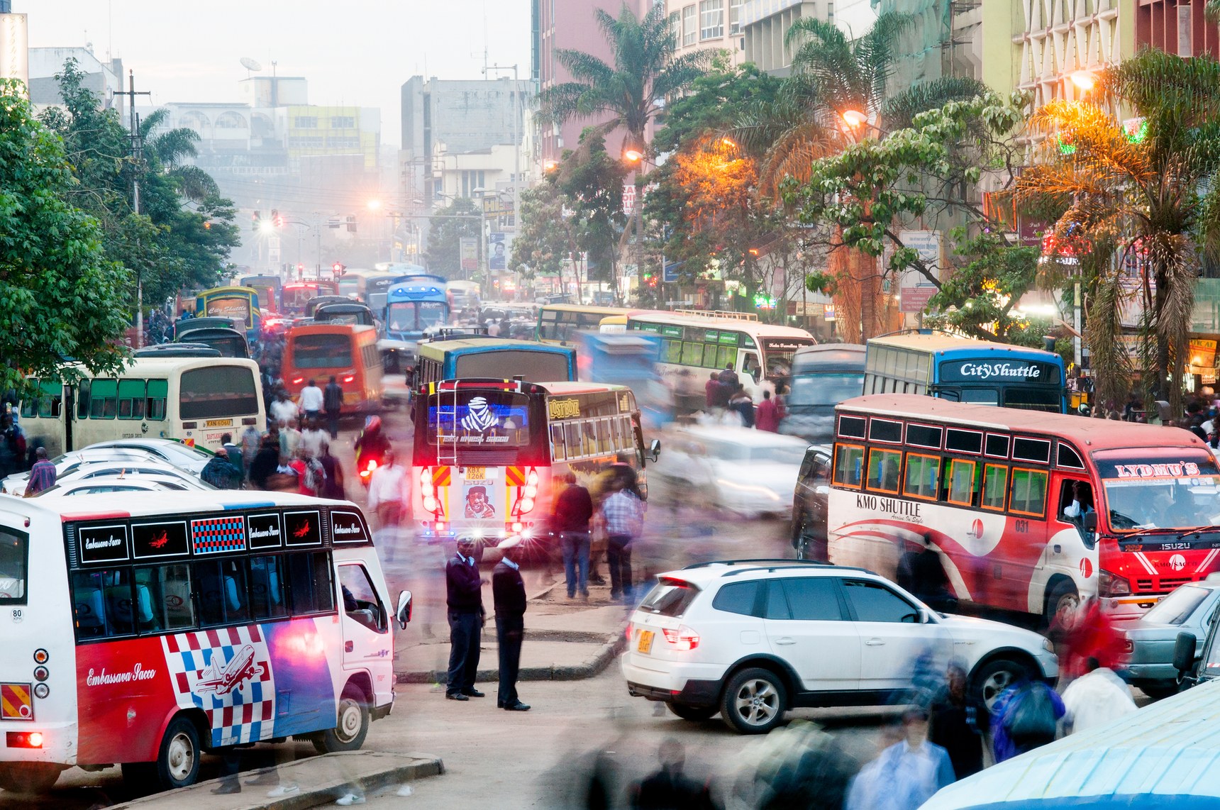
Figure 3: Peak hour traffic on Tom Mboya Avenue, Nairobi, Kenya [9]

Introduction

The Kenyan capital city Nairobi streets are famous for celebrities faces like Bob Marley or Tupac Shakur, their roads are bright and loud, blaring with car music that are honking their way through congestions. The mini bus network that is popular with 70 percent of the population of the city is known as Matatu buses. Induvial matatu buses are privately owned and run which means, there is no structure or plans for scheduling bus timings, ticket prices or route changes. This leads to long delays for passengers who accidently get on the wrong bus or tourist who are new to the city. Furthermore, as most routes run through the city centre causing bus congestions and even minor accidents can cause traffic delays for hours due to congested roads. To tackle this challenge, a collaboration was done between researchers from MIT, Columbia University and the University of Nairobi to design a transit mapping system for the Matatu bus network and launch it on Google Maps as a non-formal transit systems. This would allow residents of Nairobi to check their bus journeys using their smart phones. Two researches from the Columbia Centre for Sustainable Urban Development, Sarah Williams and Jacqueline Klopp connected with Group shot co-founder Adam White to kick start this project in 2012 and called it the Digital Matatus.

Finding a Solution Using GPS Data

The crucial element to plan the route needed the buses data however, the city government only had 75 percent of the digital Matatus records and even those only included start and end points, making it impossible to know the full bus routes through the city centre. To tackle this, ten university of Nairobi students were employed to spent four months riding the Matatus to record names and locations of each stop in a purpose-built GPS route tracking app. With the student’s efforts, almost 3000 stops on more than 130 routes were recorded and complied into a usable format called General Transit Feed Specification (GTFS). GTFS format was chosen because it is compatible with Google Maps and could easily be integrated in its transit system. Furthermore, the Digital Matatus team wanted to visualise the entire matatu transit system onto one paper map. By plotting the GPS coordinates, they could generate neuron-like mass of overlapping routes and colours. Designers at the MIT Civic Data Design Lab, started separating and structuring that neuron mass to give design a formal subway-style map, each main corridor going through the city centre was given a different colour and well-known landmarks of the city were highlighted with bright colours on the map. Both the GTFS transit data and the routes paper maps were released by the digital Matatus team in January 2014.

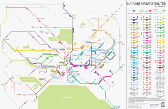
Figure 4: The official Matatu map of Nairobi developed by the project team [8] In a years’ time, the innovative tech community of Nairobi, produced five routing applications for smartphones and a payments application that calculated ticket prices for the customers journey to combat price fluctuations and fraud. More routes were added specially to underserved areas and alternative route options were then available to avoid traffic congestions.

Summary

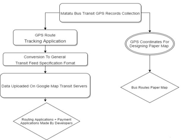
Figure 5: Block diagram summarising the Nairobi bus network case study

Conclusion and linked to the project

Public bus networks are one of the most crucial public services required for any major city, this case study shows how a cripple buss network can paralyse the lives of its citizens and affect the economy of the country. The root cause of this mismanaged network, is found to be insufficient bus transit records (data sets). Hence, the key task was to collect this crucial transit data of each bus stop so it could be processed into a usable format. Developers and other government services, can then harness this useable data sets to find solutions. This case study is a good example for our final year project because, it links well with our overall aims of optimising open data to improve transport services across the globe. It explores the different analytical techniques of collecting data sets and translating them into GTFS formats for usability. It also shows the various functionalities, i.e. paper base route maps, smartphone applications and ticket payment applications, that can be achieved from these data sets once they are in the correct format.

2.2 Shortest Path Algorithms Overview

Algorithms are tools to solve a problem in a systematic way by breaking them to smaller executable blocks.  From finance, economics to transports, logistics and engineering; the shortest path algorithm has countless applications in all major industries and fields. It comprises of finding a path between two vertices in a graph such that the total sum of the edges weights is minimum. There are various algorithms that can perform this including, Bellman Ford’s, Floyd- Wars hall’s and Dijkstra’s algorithm. In the next section, we will explore the Dijkstra’s algorithm in detail and review a case study that constructs an applications in Python that runs on the basis of this algorithm.

Dijkstra’s Shortest Path Algorithm

Dijkstra Algorithm was developed by a Dutch computer scientist Edsger Dijkstra in 1959 for finding the shortest path from node A (starting node), to the target node in a weighted graph. A weighted graph refers to an edge-weighted graph where each edge of the graph has a weight or value. The algorithm functions by first creating a tree of shortest paths which is then connected to the source and all other points in the graph. This graph can be either directed or undirected and all the edges of the graph need to have a nonnegative weight.

Problem: Finding shortest route manually using mental calculations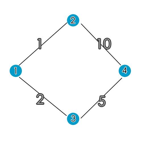

Figure 6: Simple graph to understand basic of Dijkstra’s algorithm To understand the basics of Dijkstra’s algorithm, we can start with a simple routing graph shown in figure 5.  The blue circles represent ‘nodes’ and black lines are edges or ‘node paths’. Each node has a weight (cost in Pounds’ Sterling for example) highlighted in grey. The question is to find the most cost efficient route from node 1 to node 4.

Solution

The shortest and cost effective path to reach node 4 is from node 1 to node 3 to node 4. This way it cost £2+£5= £7, compared to going from node 2 to node 1 to node 4 costing £1+ £10 = £11. This example is very easy to figure out mentally due to the small numbers and less routes involved but our goal here is to translate the steps thought in our mind into steps that a computer can follow.

Understanding the theory of Dijkstra algorithm through an example

Aim:

To find the shortest path from A to every other vertex

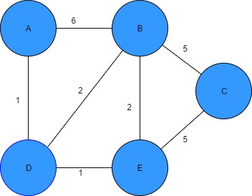
Figure 7 Finding the shortest path

Step 1

• Draw a table to layout the vertex and its distances from each node.
• Distance to A from A= 0
• Distances to all other vertexes from A is unknown therefore set to Infinity

Table 1: Dijkstra algorithm parameters

Vertex	Shortest distance from A
A	0
B	∞
C	∞
D	∞
E	∞

Step 2

• Start with the current Vertex A and visit its closet neighbours
• Current vertex is A and its unvisited neighbours are D and B
• A- D distance = 1
• A- B distance= 6
• Calculate the distance from each neighbour from the start vertex A
• If the calculated distance of a vertex is less than the known distance, update it
• Insert a previous vertex column in the table
• Visited vertexes = [A], Unvisited = [B, C, D,E]

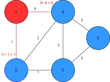
Figure 8: Finding the shortest path from node A to D & B Table 2: Dijkstra algorithm parameters

Vertex	Shortest distance from A	Previous vertex
A	0
B	6	A
C	∞
D	1	A
E	∞

Step 3: Iteration 1

• Start with the unvisited vertex with the smallest known distance from start vertex
• Our current vertex is D and its unvisited neighbours are B and E
• D- B distance = 2
• D- E distance= 1
• Calculate the distance D to neighbour B and E
• the calculated distance of a vertex is less than the known distance, hence update only B from 6 to 3
• Update the previous vertex column for B and E
• Visited vertexes = [A, D], Unvisited = [B, C, E]

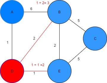
Figure 9: Finding the shortest path from node D to B & E Table 3: Dijkstra algorithm parameters

Vertex	Shortest distance from A	Previous vertex
A	0	-
B	3	D
C	∞	-
D	1	A
E	2	D

Step 4: Iteration 2

• Start with the unvisited vertex with the smallest known distance from start vertex
• Our current vertex is E and its unvisited neighbours are B and C
• E- B distance = 2
• E- C distance= 5
• Calculate the distance of E to neighbour B and C
• The calculated distance of a vertex is less than the known distance, hence update only C from infinity to 7
• Update the previous vertex column for C only
• Visited vertexes = [A, D, E], Unvisited = [B and C]

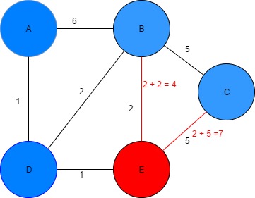
Figure 10: Finding the shortest path from node E to B & C Table 4: Dijkstra algorithm parameters

Vertex	Shortest distance from A	Previous vertex
A	0
B	3	D
C	7	E
D	1	A
E	2	D

Step 5: Iteration 3

• Start with the unvisited vertex with the smallest known distance from start vertex
• Our current vertex is B and its unvisited neighbour is C
• B- C distance = 2
• Calculate the distance of B to neighbour C
• Calculated distance of a vertex is not less than the known distance, do not update C
• No update for the previous vertex column required
• Visited vertexes = [A, D, E, B], Unvisited = [C]

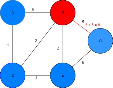
Figure 11: Finding the shortest path node B to C Table 5: Dijkstra algorithm parameters

Vertex	Shortest distance from A	Previous vertex
A	0
B	3	D
C	7	E
D	1	A
E	2	D

Step 6: Iteration 4

• Start with the unvisited vertex with the smallest known distance from start vertex
• Our current vertex is C and has no unvisited neighbours
• Visited vertexes = [A, D, E, B, C], Unvisited = []

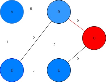
Figure 12: Finding the shortest path node C Table 6: Dijkstra algorithm parameters

Vertex	Shortest distance from A	Previous vertex
A	0
B	3	D
C	7	E
D	1	A
E	2	D

Conclusion

Following the six steps detailed above, we can summarise them into a Dijkstra Algorithms inside a repeat loop.

1. Let distance of start vertex from start vertex = 0
2. Let distance of all other vertices from start = infinity

Repeat (inside loop)

3. Visit the unvisited vertex with smallest known distance from the start vertex
4. For the current vertex, examine its unvisited neighbours
5. For the current vertex, calculate the distance of each neighbour from start vertex
6. If the calculated distance of vertex is less than the known distance, update the shortest distance
7. Update the previous vertex for each of the updated distances
8. Add the current vertex to the list of visited vertices until all vertices visited

Dijkstra algorithm for solving more complicated graphs

Aim:

To fully understand and appreciate the power of Dijkstra algorithm, we can apply it to a more complicated graph such as shown in figure 10 to find the most cost effective path from A to B.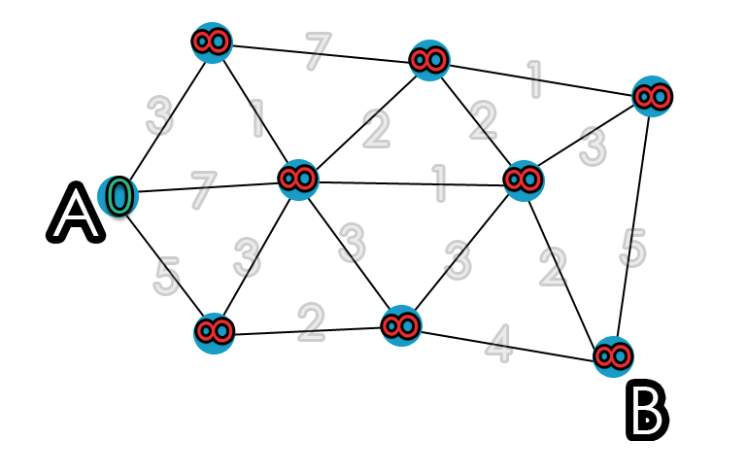

Figure 13: Dijkstra’s algorithm graph [10] Key

• C (A) = cost of A
• C (x) = current cost of reaching node x
• Grey nodes = cost of the path, temporary

Step 1: Assigning parameters

• C (A) = 0 (Starting point)
• C (x) = infinity (Every other node)

Step 2: Start the algorithm

• Start with the current Vertex A and visit its closet neighbours
• Calculate the cost to get to the adjacent nodes
• For the first node, adjacent to A, 0 + 3 = 3
• For the second node, adjacent to A, 0 + 7 = 7
• For the third node, adjacent to A, 0 + 5 = 5

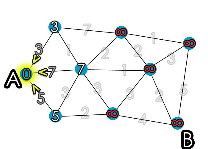
Figure 14: Calculating the cost of the first 3 nodes [10] Step 3: Iteration in a loop

• Small temporary value of C(x) = 3 so make it permanent
• Repeat the cost calculation process until left with no temporary nodes

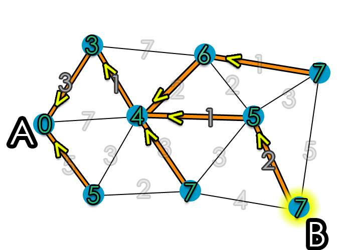
Figure 15: Final route path showing most cost-effective routes from A to B for each node [10]

2.2.1 Creating a route planner in python for California’s road network using Dijkstra algorithm

[Cyrille Rossant, Packt publishing, 2014 [11]]

Introduction

California has claimed the spot of having the worst traffic of any metropolitan area since 2015. Drivers of Los Angeles- Long Beach Santa Ana region are stuck on freeways for more than 81 hours a year, hence traffic remains a top concern for any Southern California residents, leaving even personal safety and housing cost behind according to a LA times poll [12].

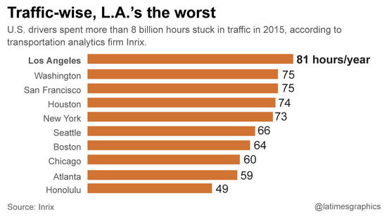
Figure 16: L.A tops US worst city for Traffic [12] This case study tries to find a solution to this traffic problem by developing a GPS-like route planner using Python programming language. By applying the Dijkstra algorithm, it can find the shortest pathway available for drivers driving on California’s busy road networks.

Specification

Table 7: Programming packages/ libraries required to create this program on Python version 2.7

Programming packages/ libraries	Short Description
Ipython	A command shell for interactive computing for Python programming environment
NumPy	For scientific computing with Python because of its powerful N-dimension array object and broadcasting functions
Pandas	Use for data manipulation and analysis by offering data structures and operations to manipulate numerical tables and time series
Matplotlib	Provides object-oriented API for adding plots into Python applications, using GUI toolkits like wxPython, QT and GTK+
Network X	For creating or manipulating structures, dynamics and functions of complex networks
GDAL/ OGR	Translator library for single raster and vector geospatial data formats into abstract data models
Smopy & Pillow	Creates an OpenStreetMap tile image when given the correct geographical coordinates (Latitude/Longitude) and a zoom level to display

Data File Description

The data used to run this program comes from the United State Census Bureau website which holds open data sources for the entire US economy and people. It is managed by the US. Department of Commerce which has headquarters in Suitland MD since 1942 [13]. The data file is in shapefile (SHP) format which is popular with geospatial vector data sets hence, we require the GDAL and network X libraries (table 9) to extract this file in our program. Using a shape file viewer application, we can view the contents of the data set, a small extract is shown in Table 8: Extract of contents of the SHP data file

	Full Name	MTFCC	RTTYP	Distance
0	State Rte 1	S1200	S	100.658130
1	State Rte 1	S1200	S	33.419556
2	Cabrillo Hwy	S1200	M	4.399051
3	State Rte 1	S1200	S	12.400382
4	Cabrillo Hwy	S1200	M	36.693272

MTFCC is a classifier abbreviated for MAF/TIGER Feature Class code that the Census Bureau use to classify and describe their geographical positions. RTTYP is the route type code that describes the six different types of roads.

1. County - C
2. Interstate - I
3. Common Name - M
4. Other – O
5. State recognised - S
6. U.S. – U

Running the program

Once the file has been extracted using the ‘‘read_shp’’ command, they connect the different nodes together to compute the shortest path using ‘‘connected_componenet_subgraphs’’ function.  They then define the Latitude and Longitude coordinates to find the shortest path between them.

• Position 1: (36.6026, -121.9026) – Location point in Monterey, CA USA
• Position 2: (34.0569, -118.2427) – Location point in Los Angeles, CA USA

This program is based on Dijkstra algorithm therefore each edge of the node contains information (weight) about the roads. A function that returns an array of coordinates for all edges in the graph was created, furthermore, functions for calculating distances between the coordinates, computing its length and attributing the distances to the edges followed. This section of the code was then ended with writing a function that finds the two nodes in the graph that are closest to the specified latitude/ longitude coordinates and implementing the Network X shortest_Path function that is based on Dijkstra algorithm to run the iterations. The weight of every edge was specified as the length of the road between them. To develop a graphical user interface to map the coordinates, they use Smopy library to retrieve a map base tile from Open Street Map directories. The path on the map should contains connected nodes in the graph with every node characterised by a list of road points. To concatenate these positions along every edge of the path, they order the positions of the road points as the last point in an edge being close to the first point in the next edge.  The paths are then converted to pixels and displayed on the Smopy map show the final program in Figure 17.

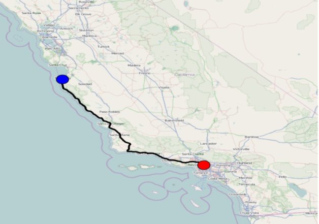
Figure 17: Output and result in graphical format

Summary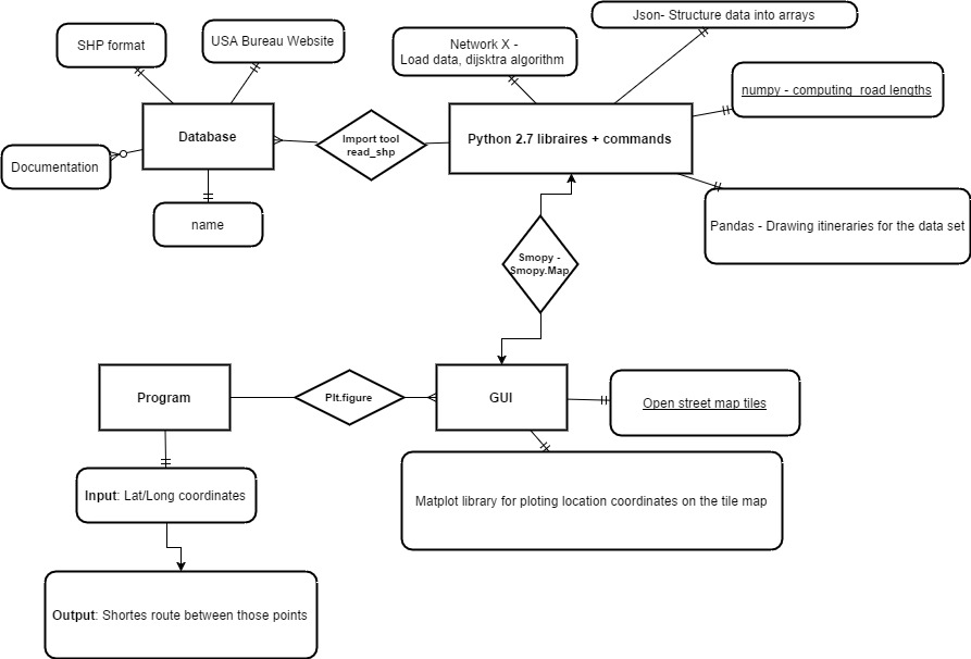

Figure 18: Block diagram summarising the California route planner case study  

Conclusion and linked to our project

This case study attempts to solve a real-world traffic congestion problem by developing a Python base route map application that draws the shortest path between point A and B. It runs on the bases of Dijkstra algorithm which was explored earlier in this section, and utilises various data sets, python functions and libraries which are summarised in figure 18 to construct the final application. It is beneficial for our final project because, we will also be utilising a few of the plotting libraries including, Numpy, Pandas and matplot.lib like this program. The data calling syntax and function would be different because our files are in different formats however, the methodology is similar. This program calls on latitude/ longitude coordinates to construct its path, similarly for our own program, we will also be inputting GPS Lat/long coordinates and hope to output optimum routes between those points. This case study uses ‘‘Smopy’’ libraries to construct their map’s however, we will be using matplot.lib and it’s basemaps for our results visualisation.

2.3 Travelling Salesman Problem (TSP)

Overview

One of the most famous computer science problems, TSP is an intuitive way of finding the shortest possible route, given a list of addresses and their pairwise distances, in a logical manner which encompasses of visiting each address exactly once and return to the original address when finish.

Example

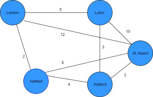
Figure 19: List of towns for TSP algorithm to find the optimum path

Problem: Salesman starting from London must pass through all cities only once to deliver his product and then returns to London at the end of his shift therefore, he needs to find the shortest route possible that covers all vertices in the graph figure 17.

Solution:  These are the few paths that the salesman can take.

• Path 1 = {London, Hatfield, Watford St Albans, Luton, London} = 2+4+3+10+5= 24
• Path 2 = {London, Hatfield, Watford, Luton, St Albans, London} = 2+4+3+10+12 = 31
• Path 3= {London, Hatfield, St Albans, Watford, Luton, London} = 2+8+3+3+5 = 21

Hence, Path 3 would be the most optimum route that our sales man can take to cover all towns and return to London in the shortest duration. There are various algorithms that solve the TSP problem, we will explore a few popular one’s before reviewing a case study that utilises this technique to solve a real-world problem.

1. Hamiltonian cycle

This theorem states that the travelling salesman problem is ‘NP- complete’. NP stands for non-deterministic polynomial time, which means that the problem can be solved using non-deterministic Turing machine. NP- Hard/complete, are classes of problems that cannot be solved in realistic time. There are usually approximation solutions that give approximation bounds. These are special notations that measure how close the approximation is to the real solution. Coming back to the theorem, we first prove that TSP belongs to NP by checking that our tour contains each destination once. Sum the total distances of the edges and check if its minimum, this way it can be completed in polynomial time and belong to NP. Second step is to prove that TSP is NP- complete. To do this we show that Hamiltonian cycle is ≤ TSP. We start by constructing an equation for Hamiltonian cycle as shown in equation (1).

G=(V, E)

(1)

Our TSP equation (2) would be;

G'=V, E'

(2)

To create the complete graph using equation (2), we need to initialise E’ as shown in equation(3).

E'=i,j:i,j∈V   i≠j

(3)

The cost function t(i,j)would be defined as shown in equation (4)

ti,j={0 if i,j∈E1 if i,j ∉E}

(4)

Hamiltonian cycle hexist in Gand the cost of each edge in his 0. Therefore, when each edge belongs to Ein G’, the cost of h will be 0 in G’. This means that when the graph Ghas a Hamiltonian cycle then the graph of G’will have a tour cost of 0. Furthermore, we assume that G’has tour h’of cost 0 and the cost of edges in E’are 0 and 1. Therefore, as the cost of h’is 0, each edge will also have a cost of 0. Hence, we can conclude that h’contains edges only in Eand can now prove that Gcan have a Hamiltonian cycle when G’has a tour cost of 0 thus, TSP is NP- complete [14].

2. Greedy Algorithm for TSP

This is a simple improvement algorithm which starts with a departure node 1, calculates all the distances to the other n-1 nodes. Goes to the next closest node before recording the current node as the departure node and then selecting the next node from the remaining n-2 nodes. The cycle then repeats until all nodes are visited only once and then ends back to Node 1 in a close loop, this gives the optimum shortest route which passes through all nodes. Advantages of this algorithm is its simplicity to understand and implement. It works well when the problem size is small and has less computational time [15].

3. 2-Opt Algorithm

When we have n-nodes for our TSP problem, we can use this algorithm which consist of three steps. Step1 

1. Let s be the initial solution that’s provided by the user
2. Let z be the objective function value
3. Set the following
   • S*= s
   • Z*=z
   • i=1
   • j=i+1=2

Step 2

1. Set S’ = Z’ < Z*
2. Z*=Z’
3. S*=S’
4. If j < n,
   • Repeat step 2
5. Otherwise, set the following
   • i= i+1
   • j=i+1
6. If I < n
   •  Repeat step 2
7. Otherwise
   • Go step 3

Step 3

1. If S≠S*, Set the following
   • S = S*
   • Z= Z*
   • i=1
   • j=i+1=2
   • Go to step 2
2. Otherwise,
   • S* the best solution and terminate the process

Explanation

This algorithm works by transposing nodes 1 and 2 to see if their results are smaller than the initial solution, so they can be stored for future consideration. Else, if the results are bigger, they are discarded and the algorithm repeats by transposing nodes 1 and 3. If this exchange generates an optimum solution, it is stored and any previous solutions are discarded. This process continues until all pairwise exchanges of the nodes are considered by the algorithm. Each node can be exchanged with n-1, there are n nodes in total, therefore, n(n-1) can be divided by 2 different exchanges. This exchange is seen in step 2, where the solution retained at the end is considered as the most improved. The algorithm then takes this solution to find if there are any more improvements possible, if not the algorithm displays this solution as the best option to the user and terminates the process [15].

2.3.1 Mapping Langkawi Tourist Destinations Using Travelling Salesman Application

[Zakiah Hashim and Wan Rosmanira Ismail [16]]

Introduction

Langkawi Island is one of Asia top tourist attractions visited by millions of visitors every year. In 2014 Langkawi welcomed around four million tourists to its beautiful white sand beach resorts, world famous amusement parks and land marks [17]. With more than thirty tourist places on offer with various attractions, it can be difficult for tourist to decide which places to visit specially if they have a tight holiday schedule or budget. This case study focuses on solving this routing problem by using the travelling sales man (TSP) optimisation tool for to map the optimum holiday tour package. It considers 19 of the most attractive tourist spots recommended by the Ministry of Tourism Malaysia website and those which can be reached via ground transportation and road networks as the study is based on self-drive tours. Table 9: Estimated trip time in minutes to visit the 19 tourist destinations

Tourist Destinations	Abbreviations	Travel timing (min)
Eagle Bay	DL	30
Taman Lagenda	TL	90
Langkawi Crystal	KL	60
Mahsuri Mausoleum	MM	90
Kampung Buku Malaysia, Langkawi	KBL	90
Underwater World	UW	120
Pantai Chenag	PC	120
Paddy Rice Museum	LP	90
Field of Burnt Rice	BT	30
Oriental Village (Langkawi Cable Car)	OV	150
Seven Walls Waterfalls	TT	150
Crocodile Farm	TB	120
Temurun Waterfall	ATT	150
Langkawi Craft Complex	KKL	90
Air Hangat Village	TAH	120
Tanjung Rhu	TR	90
Galeria Perdana	GP	90
Mount Raya (Gua Cherita)	GR	90
Langkawi Wildlife Park	ZM	120

Parameters for The Travelling Sales Man

Problem

To develop the mathematical model of TSP, first the major parameters were set.

1. Total time for travelling and visiting in a day was set to 10 hours based on the operation hours (8.00 to 18.00) of majority of the tourist destinations in the table 1.
2. The estimated travel time and the distance between the origin and destination were obtained using Google Maps for each selected path.
3. The prices of petrol for the cheapest fuel on the market, RON95 Petrol type was used at RM1.95 per litre. The average consumption of 1 L of petrol is 10 km hence, the fuel cost per kilometre is RM 0.195.
4. Car rental estimated cost per day (24 h) is RM 134.00
5. Neatest accommodation within 5 Km radius of the tourist spot visited on that day with the lowest price was selected to stay in for the night.

Mathematical formulation

Ferry ride is the major transportation hub used by tourist to reach or exit Langkawi island therefore, Kuah Jetty (JK) was used as the deport (first and last destination for visiting all the 19-tourist spot) in developing the TSP model.

Minimise:   ∑i=jn∑j=1ndij Xij600

(5)

∑i-1nxij=1;   j=1,2,…,n,   i≠j

(6)

∑j-1nxij=1;   j=1,2,…,n,   j≠i

(7)

ui-uj+nxij- ≤n-1;   i≠j;i=2,3,….,n;  j=2,3,…,n

(8)

xij ∈0,1;  ∀ij=1,2,…,n

(9)

Key

• dij= Travelling and visiting time (in minutes) from tourist destination i to tourist destination j.
• ui= Sequence number of tourist destination i on the trip.
• uj= Sequence number of tourist destination j on the trip.
• xij={1=For path from tourist destination I to j}
• Xij= {0= Otherwise}

Explanation for each equation

1. Minimising tool for total travelling and visiting time for 1 day, 10 h (600min)
2.  Constraint for tourist arriving only once for each destination
3. Constraint for ensuring tourist leaves each destination once
4. Constraint to avoid sub-tours.

Results

To solve the mathematical formulation listed above, LINGO version 12.0 was used as it’s a faster, easier and effective modelling tool commonly used in the industry to solve TSP. The final optimum route which encompasses all 19 tourist destinations is the following:

JK → DL → TL → TAH → GP → TR → KKL → TB → ATT → OV → TT → BT → LP → PC → UW → MM → GR → KBL → ZM → KL → JK

It would take 4 days to travel all the 19 destinations according to the 10 hour (600min) per day visiting time restrictions. After reaching the destination in the allocated time for each day, the tourist will need to find the nearest accommodation (less than 5 km) with the lowest price to stay for that night.  For this case, three different hotels will be selected for four days because for the last day visit, tourist will leave Langkawi Island without staying in the hotel.  The whole pathway, including the cost of each day and the total cost of the trip is shown in the table 2 below. Table 10: Solution to find the optimum travel route

Day	Path	Travel Cost between destination (RM) A	Accommodation Cost (RM) B	Car Rental Cost (RM) C	Daily Total Traveling Cost (RM) A+B+C
1	JK → DL → TL → TAH → GP → TR → KKL	0.05 + 0.20 + 0.31 + 0.99 + 2.28 + 1.54 = 5.37	82.00	134.00	221.37
2	KKL → TB → ATT → OV	2.32 + 1.23 + 2.77 = 6.32	150.00	134.00	290.32
3	OV → TT → BT → LP → PC → UW	0.23 + 2.30 + 1.77 + 0.18 + 0.13 = 4.61	60.00	134.00	198.61
4	UW → MM → GR → KBL → ZM → KL → JK	2.50 + 4.25 + 3.16 + 1.74 + 0.23 + 0.37 = 12.25	0.00	134.00	146.25
Total travelling cost (RM): 856.55

Summary

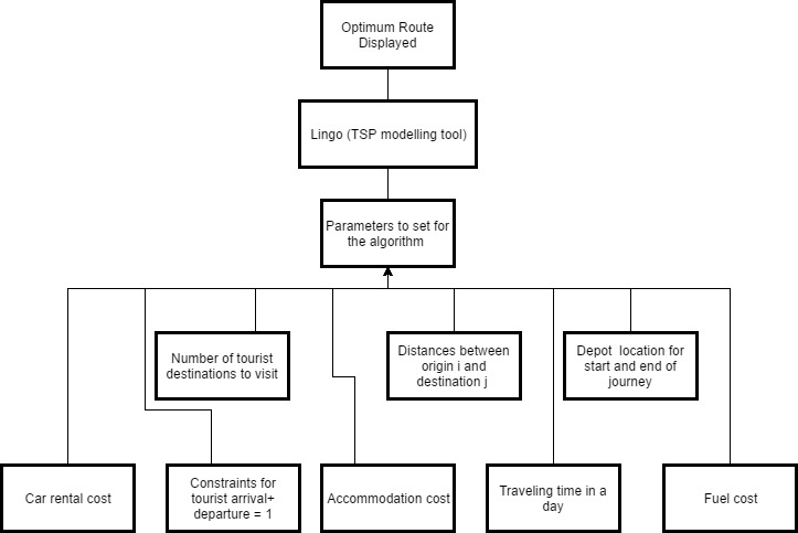
Figure 20: Block diagram for the shortest tourist destination routes for the TSP case study

Conclusion and linked to our project

We can see that the proposed TSP model is proven successful in providing tourist with a suitable path for visiting popular tourist destinations in Langkawi. Tourist can save up to RM 334.55 because the regular path would cost an individual RM 1191.10 as opposed to RM 856.55 generated from the TSP model.  This case study is very beneficial for our final project because it gives an understanding of implementing the TSP optimisation tool, discussed earlier in this section, to real world transport problems. Our final project will also be utilising the TSP algorithms to map the optimum routes for our different UK city coordinates. Similar parameters such as, start and stops location, distance between locations, travelling times and number of destinations, will dictate the outcome of our program. The final version will be presented on a visual world base map graphical interface.

3 Description of the Project Work

This section will highlight all the various stages of work that were undertaken in developing our route planner application. It will talk about the various methodologies that were investigated for data analytics, algorithm implementations and results visualisation.

3.1 Stages of work

The aim of this project was to develop a route planning application that can calculate the shortest path between different nodes (locations) using GPS location coordinates. These coordinates were obtained from Open Data files. The project commenced in October 2016 of our final year of Undergraduate Engineering degree and had a seven-month time line, finishing in April 2017. In the next few subheadings, we will discuss the various stages and challenges involved in this project, from the initial planning stage, to the design and implementation of the software algorithms and testing the results to analyse and validate our application.

Stage 1: Planning

This staged involved background research into Open Data and its applications. We started by understanding what is Open Data, who can have access to it and what benefits it brings to the users. The case studies discussed earlier in the literature review, were analysed in detail to help further enhance our understanding of the topic specially in relation to the transport sector.  We then started to downloaded different static data sets from various sources including, Data.Gov.UK, Data.Gov.SG (Singapore open data source) to analyse its content and usability. We also considered real time live data streams known as Application Programming Interface (API) feed from sources including TFL and UK Highway Agency. The aim was to strengthen our data analytic skills by understanding the various elements of the data files and selecting the useful features (contents) from those files for our final project. Figure 21 show’s a screen shot of one of the data files that we analysed in the early planning stages of our project. This data set which was in CSV format was downloaded from the DATA.GOV.UK. It shows the number of vehicles counted at specific location across the UK between 2009 to 2013 and was collected on an annual basis using video surveillance technology. By analysing this data set the important rows we concentrated for our transport problem included, road numbers, names, dates, all vehicle flow and the Easting/ Northing coordinates. HGV_Flow and Bus_Coach_flow columns could be discounted at this stage because we are not classifying what specific vehicle are on the road but a general view of traffic flow.

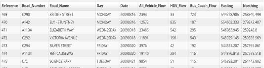
Figure 21: Example of data files analysed for improving data analytic techniques

Our project is entirely software base therefore, one of the major tasks was to choose a powerful programming language that would be best suited for processing data analytic algorithms and could also developed web applications, incorporating static algorithmic codes into production data base and having data handling /visualisation capabilities. We compared two major contenders in the programing world for this job, MATLAB and Python, table 11 below shows the comparison made between them which helped derive the conclusion for our choice. Table 11: MATLAB vs Python programing language [18]

MATLAB	Python
Numerical computing environment and programming language	Programming language that is related to C and consist of extensive library database
Cost is considerably high for full version and the basic student version available is £29	Free download from Python.org for the full version
Generic libraries do not contain a lot of generic programming functionalities and the data process, plotting and visualisation libraries are only included in the extensive version which cost more money	The generic libraries are aimed at high level programming and contain modules for os specific stuff, thread, networking, databases all included in the free version
There’s toolkit provided by Math work to perform high level scientific computing but cost extra money	To perform scientific computing, additional packages including Numpy, Matplotlib or Scipy must be download. An easier way to get hold of all the major scientific libraries of python is through downloading Anaconda free of charge from theAnaconda Continuum Analytics website
The algorithms are proprietary which means they are hidden in the background and have portability restriction which stops it from running on someone else’s computer. Complied application can be run using the MATLAB Component Runtime (MCR) but portable apps must exactly match the version of the installed MCR on the other person’s PC. This can be a nuisance because MATLAB releases a new version every Six month on average. This also make it very difficult for Third party to develop packages for extending MATLAB’s functionalities.	Because of its open and free source nature, it can benefit from other Third parties to design packages or software tools that extend its capabilities. It has a high portability rate because its code can run from one platform say Windows to the other- Linux, without downloading any further compatibility tools.  It is very powerful in creating front-end interfaces for high end applications because of it’s an extensive GUI toolkit library which includes, WX, Qt and Pyzo.

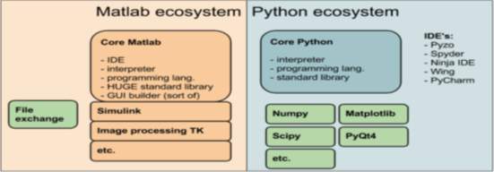
Figure 22: Illustrating the differences between the two ecosystems [18] Therefore, Python programming language fulfilled all our criteria’s and was chosen as our primary language to develop the application for our project.

Stage 2: Design and Implementation of the Software Algorithm

The core engine of our application runs on the short path algorithms which calculates distances between different locations to map the shortest path between them. We started by researching into various shortest path algorithms including, Bellman Ford’s, Dijkstra and Travelling Salesman Problem. In the literature review section, we have discussed the Dijkstra and TSP algorithms in detail with the case study examples as they are very relevant in developing the architecture of our own application. Various algorithms were tested to implement in our programme including the Dijkstra’s California route planner case study. However, passing GPS coordinates into the code is difficult because it is built around passing SHP File Format Data Sets which are difficult to open using normal file viewers. Also, the code is………. The main algorithm was taken from the Google optimisation tool for

References

[1] Open Data Institute, “Guides- What make data open?,” 2016. [Online]. Available: https://theodi.org/guides/what-open-data.

[2] Open Government Licence for public sector information, “Using Information under this licence,” 2016. [Online]. Available: http://www.nationalarchives.gov.uk/doc/open-government-licence/version/3/.

[3] T. Jetzek, “A framework for analyzing open public sector information initiatives,” 2012.

[4] M. A. Talaat, “Public Sector Information and Open Government Data,” Journal of systems integration (2010), 2016.

[5] Future Spaces Foundation, “Future Space Foundation,” 12 05 2016. [Online]. Available: http://www.futurespacesfoundation.org/2016/05/open-up-your-data-to-open-up-our-cities-the-future-spaces-foundation-calls-for-open-access-to-transport-data/#_ftn1.

[6] B. Hogge, “TRANSPORT FOR LONDON,” Creative Commons , 2016.

[7] L. Springthorpe, “The Big Challenges for the Next Mayor of London,” 10 January 2016. [Online]. Available: http://www.huffingtonpost.co.uk/luke-springthorpe/london-mayoral-election_b_8937652.html.

[8] S. W. A. W. XU, Artist, Matatu map of Nairobi. [Art]. MIT CIVIC DATA DESIGN LAB, 2014.

[9] T. COCKREM, Director, How Nairobi Got Its Ad-Hoc Bus System on Google Maps. [Film]. GETTY IMAGES.

[10] E. Hazzard, “Dijkstra's Algorithm - Shortest Path,” DISQUS, 22nd May 2010. [Online]. Available: http://vasir.net/blog/game_development/dijkstras_algorithm_shortest_path/.

[11] C. Rossant, “Creating a route planner for road network in Python,” in IPython Interactive Computing and Visualization Cookbook, Packt Open Source, Packt Publishing Ltd, 2014.

[12] L. J.Nelson, “Los Angeles area can claim the worst traffic in America. Again,” Los Angeles Times, L.A, 2016.

[13] United Census Bureau , “Who we are?,” 2016. [Online]. Available: https://www.census.gov/about/who.html.

[14] “The Traveling Salesman Problem,” [Online]. Available: http://www.csd.uoc.gr/~hy583/papers/ch11.pdf.

[15] J. -I. S. M. Z. Byung-In Kim, “Comparison of TSP Algorithms,” 1998.

[16] Z. H. a. W. R. Ismail, “Problem in Optimizing Tourist Destinations Visit in Langkawi,” in Regional Conference of Sciences, Technology and Social Sciences (RCSTSS 2014, Malaysia, 2014, pp. 255-272.

[17] FMT Content Partner, The Malaysian Reserve, “Langkawi targets 4m tourists by year-end,” June 20, 2013.

[18] S. H. Abbi Hobbs, “Big and Open Data in Transport,” POST, London, 2014.