The Project Proposal of Computational Simulation of Noise Propagation from A Subsonic Turbulent Jet

Table of Contents

Abstract

1 Introduction

1.1 Researches in Jet Noise

1.2 RANS model and FWH Model

2 Methodology and Research Design

2.1 Standard

k-ϵ models

2.2 RNG

k-ϵ model

2.3 Realizable

 k-ϵ model

3 Proposed Work

3.1 Work done

3.2 Work to be done

4 Project Management

5 References

 

Abstract

Jet noise is a common problem correlated with low bypass-ratio turbofan engines and turbojet engines. The research in jet noise was initiated by Sir James Lighthill in 1952 (Tam, 1998, p. 393) and his solid mathematical model of jet noise was firstly published in 1963, which includes the theories of subsonic and supersonic turbulent jet noise as well the solutions to them (LIGHTHILL, 1963, p. 1510~1515). Since the attention of aviation industry started to draw on the environmental impact, the noise generation and control of aircrafts where jet noise plays a significant role has become an active field of study over last half centuries. Nowadays, commercial aircrafts with high bypass ratio engines has improved the jet noise control based on Lighthill’s method of reducing the relative velocity of the jet and air surrounded.

This project is aiming to predict the noise propagation of a subsonic turbulent jet in the far-acoustic field. The turbulent jet is simulated based on Reynolds Averaged Navier Stokes (RANS) models and the far-field noise is computed using Ffowcs-Williams/Hawkings (FWH) model. The simulation will be conducted by ANSYS Fluent Package. The project is arranged into two sections of turbulent jet simulation and far-field noise simulation. An initial turbulent jet simulation has been conducted to validate the feasibility of the method used. The behaviour of the initial turbulent jet was compared with other experimental data and proved valid. The result of turbulent jet will be improved by applying User Defined Function (UDF) of the inlet velocity profile and any other UDFs if necessary. Further simulations on noise propagation will be conducted soon after the more convincing simulations of turbulent jet.

1        Introduction

1.1  Researches in Jet Noise

Aeroacoustics is a rather recent field of study involving both aerodynamic and acoustic phenomenon (Anselmet and Mattei, 2016, p. 7). The birth of aeroacoustics dates to 1952 when Sir James Lighthill published the first part of his On Sound Generated Aerodynamically, General Theory building up the theory of the production of aerodynamic sound (Lighthill, 1951). The second part, Turbulence as a Source of Sound specifying the research to turbulence as a source of sound and validating the theory from experimental data (Lighthill, 1954).

In 1963, Ffowcs Williams extended the theory initiated by Lighthill in 1952 to solve the transonic and supersonic eddy convection speed. The original Lighthill’s theory illustrates that the intensity of radiated noise increases with eighth power of the jet velocity, which is known as Lighthill Vj8 Law. Williams investigated that the quadrupole degenerates into simple sources whose radiation intensity increases with the third power of the jet velocity for supersonic jet (Williams, 1963). These two theories are the most important in Acoustic Analogy Theory (Tam, 1998, p. 394).

In 1970s, the discovery of turbulence in jet and free shear layer is made of both large turbulence structures and fine-scaled turbulence by several individual researchers led to the proposal of the significance of Large Turbulence Structures Model with which solely supersonic jet works (Tam, 1998, p. 395~396).

In the early 1990s, Jet Noise Laboratory of the NASA Langley Research Centre conducted high-temperature jet noise experiments with temperature ratio up to five, which offered an opportunity to validate the theory developed by Lighthill. The finding of turbulent mixing noise from both supersonic and subsonic jet has two distinct components of large turbulence and fine-scaled turbulence was addressed and validated.  (Tam, 1998, p. 398~401).

Since the technologies of computing and programming were developed rapidly in eighties and nineties, computational methodologies were introduced in all kinds of fields. Computational Aeroacoustics is a useful tool to assists on the researches of jet noise in terms of obtaining reliable computational results before conducting costly experiments as well as efficiently proving hypothesis.

1.2  RANS model and FWH Model

For Linear Eddy Viscosity Model, the governing equation of RANS model (Tucker, 2008, p. 99)given below is deducted by averaging the Navier-Stokes equation:

	∂ui∂t+∂uiuj∂xj=-1ρ∂p∂xi+μρ∂∂xj ∂ui∂xj+∂uj∂xi+1ρ∂τij∂xj	(1.1)

This turbulence model is applied to estimate the Reynolds stress term:

	∂τij=(-ρui’uj’̅)	(1.2)

The Boussinesq approximation is applied:

	-ρui’uj’̅=2μtSij-23ρkδij	(1.3)

Note that

μtis the turbulent viscosity, also known as eddy viscosity.

δijis the Kronecker delta in which

δij=1if

i=jand

δij=0if

i≠j. The mean turbulent kinetic energy has the form of

k=12u1u1+u2u2+u3u3. The inclusion of

23ρkδijis required later in the two-equation

k-εmodels. The mean strain rate

Sijis given by:

	Sij=12∂ui∂xj+∂uj∂xj	(1.4)

Considering the large amount of time potentially taken if the methods of high-order equations are used in this project, only the two-equation

k-ϵmodels will be used to conduct simulations. In this case, the turbulent jet is assumed to be symmetrical. The details of

k-εmodels will be discussed in following section.

FWH model is based on the equation extended from Lighthill’s volume integral, where the model predicts far field sound form a flow region,

V, close to a moving surface,

s.

Based on the finding in ANSYS User Guide and the paper of Brentner and Farassat (Brentner and Farassat, 1998; ANSYS.Inc, 2009) FWH equation can be expressed in the form of a inhomogeneous wave equation:

1a02∂2p’∂t2-∇2p’=∂2∂xi∂xjTijHf   -∂∂xiPIJnj+ρuiun-vnδf +∂∂tρ0vn+ρun-vnδf

(1.5)

To define the components in equation (1.5).

uiis the fluid velocity component in the

xidirection,

unis the fluid velocity component normal to the surface where

f=0and they have corresponding surface velocity components

viand

vn. The

δfis the Dirac delta function and

Hfis the Heaviside function.

p’is the sound gauge pressure at the far field.

The Lighthill stress tensor is defined as:

	Tij=ρuiuj+Pij-a02ρ-ρ0δij	(1.6)

Note that

a0is the far-field sound speed.

Pij

is the compressive stress tensor:

	Pij=pδij-μ∂ui∂xj+∂uj∂xi-23∂uk∂xkδij	(1.7)

Note that it is not necessary for the surface

f=0coincide with the physical body surface. This is demonstrated in the paper of Brentner and Farassat (Brentner and Farassat, 1998, p. 3) and ANSYS allows the source surfaces to be placed in the interior of the flow.

2        Methodology and Research Design

2.1  Standard

k-ϵ

models

Firstly, the standard

k-ϵmodel (Launder and Spalding, 1972) is introduced in which the assumptions of fully turbulent jet and negligible molecular viscosity are applied for this method. There are two transport equations governing the standard

k-ϵmodel.

For turbulent kinetic energy

k:

	∂∂tρk+∂∂xiρkui=∂∂xjμ+μtσk∂k∂xj+Pk+Pb-ρϵ-YM+Sk	(2.1)

For dissipation

ϵ:

	∂∂tρϵ+∂∂xiρϵui=   ∂∂xjμ+μtσϵ∂ϵ∂xj+C1ϵϵkPk+C3ϵPb-C2ϵρϵ2k+Sϵ	(2.2)

Note that

Skand

Sϵare User-Defined sources.

The turbulent viscosity is modelled in the form of:

	μt=ρCμk2ϵ	(2.3)

The turbulence kinetic energy generated due to mean velocity gradients,

Pk:

	Pk=-ρui’uj’∂uj∂xi=μtS2	(2.4)

where

Sis the modulus of the mean rate of strain tensor:

	S≡2SijSij	(2.5)

The turbulence kinetic energy generated due to buoyancy,

Pb:

	Pb=βgiμtPrt∂T∂xi	(2.6)

where

Prtis the turbulent Prandtl number for energy and

giis the component of the gravitational vector in the

ith direction.

βis the coefficient of thermal expansion:

	β=-1ρ∂ρ∂Tp	(2.7)

YM

, the dilation dissipation to the overall dissipation rate is defined as:

	YM=2ρϵMt2	(2.8)

where

Mtis the turbulent Mach number.

Note that there are several constants obtained based on experiments in the transport equations.

C1ϵ=1.44, C2ϵ=1.92, Cμ=0.09, σk=1.0, σϵ=1.3. C3ϵdetermining the level of the buoyancy effect to

ϵis rather a variable other than a constant. In ANSYS Fluent, it is defined as:

	C3ϵ=tanhvu	(2.9)

Where

vis the parallel component of flow velocity to the gravitational vector and

uis the perpendicular component of that.

2.2  RNG

k-ϵ

model

RNG

k-ϵmodel (Orszag, S. A., Yakhot, V., Flannery, W. S., Boysan, F., Choudhury, D., Maruzewski, J., & Patel, 1993) is derived by renormalizing the Navier Stokes equations by Re-Normalisation Group method. RNG

k-ϵmodel enhances the accuracy for rapidly strained flows and swirling flows from the standard one. RNG

k-ϵmodel has similar transport equations of

kand

ϵwith the standard one.

For

k:

	∂∂tρk+∂∂xiρkui=∂∂xjαkμeff∂k∂xj+Pk+Pb-ρϵ-YM+Sk	(2.10)

For

ϵ:

	∂∂tρϵ+∂∂xiρϵui=   ∂∂xjαϵμeff∂ϵ∂xj+C1ϵϵk(Pk+C3ϵPb-C2ϵρϵ2k-Rϵ+Sϵ	(2.11)

Another reason for RNG

k-ϵmodel provides higher accuracy is that it can handle both high-Reynolds-number and low-Reynolds-number conditions well.

The following differential equation is applied to obtain an accurate description of the behaviour of effective turbulent number along with the effective Reynolds number:

	dρ2kϵμ=1.72v̂v̂3-1+Cvdv̂	(2.12)

where

v̂=μeff/μand

Cv≈100.

In high-Reynolds-number case, equation (2.12) gives equation (2.3) with

Cμ=0.0845.

As mentioned above, the effect of swirl is included in RNG

k-ϵmodel. This is achieved in ANSYS Fluent by modifying the turbulent viscosity where the modification works with axisymmetric, swirling flows and three-dimensional flows.

The inverse effective Prandtl number for

kand

ϵare

αkand

αϵare respectively. They could be derived by the following equation:

	α-1.3929α0-1.39290.6321α+2.3929α0+2.39290.3679=μmolμeff	(2.13)

where

α0=1.0. As

μmolμeff≪1where the high-Reynolds-number case is applied,

αk=αϵ≈1.393.

In the transport equation for

ϵ,

Rϵcan be further defined as:

	Rϵ=Cμρη3(1-ηη0)1+βη3ϵ2k	(2.14)

and a new term

C2ϵ*is introduced:

	C2ϵ*=C2ϵ+Cμρη3(1-ηη0)1+βη3	(2.15)

so that equation (2.10) can be rearranged into:

	∂∂tρϵ+∂∂xiρϵui=   ∂∂xjαϵμeff∂ϵ∂xj+C1ϵϵk(Pk+C3ϵPb-C2ϵ*ρϵ2k	(2.16)

where

η≡Skϵ, η0=4.38, β=0.012.

Note that for weakly to moderately strained flows of

η<η0, the RNG

k-ϵmodel provides results close to those of the standard one. Whereas for rapidly strained flows of

η>η0, a smaller turbulent viscosity is obtained from RNG

k-εmodel.

The model constants are

C1ϵ=1.42, C2ϵ=1.68and

C3ϵis obtained referring to equation (2.8).

2.3  Realizable

 k-ϵ

model

The ‘‘realizable’’ of the model means that it complies with certain mathematical constraints on the Reynold stresses. Using realizable

k-ϵmodel (Shih et al., 1995) provides more accurate prediction on the spreading rate of planar and round jet as well as the steady performance for flows of rotation and boundary layer under strong adverse pressure gradients, separation and recirculation. Realizable

k-εmodel also has two transport equations.

For

k:

	∂∂tρk+∂∂xiρkui=∂∂xjμ+μtσk∂k∂xj+Pk+Pb-ρϵ-YM+Sk	(2.17)

For

ϵ:

	∂∂tρϵ+∂∂xiρϵui=   ∂∂xjμ+μtσϵ∂ϵ∂xj+ρC1Sϵ-ρC2ϵ2k+vϵ+C1ϵϵkC3ϵPb+Sϵ	(2.18)

where

C1=max⁡0.43,ηη+5.

The turbulent viscosity for realizable

k-ϵmodel is computed instead of a constant like in standard and RNG

k-ϵmodel:

	Cμ=1A0+AskU*ϵ	(2.19)

Note that

A0=4.04and

As=6cosϕ.

ϕ=13cos-1⁡(6W)and

W=SijSjkSkiS̃3.

S̃=SijSij

U*

is defined as:

	U*≡SijSij+Ωij̃Ωij̃	(2.20)

Note that

Ωij̃=Ωij-2ϵijkωkand

Ωij=Ωij̅-ϵijkωk.

Ωij̅is the mean rate-of-rotation tensor with respect of a rotating reference frame of angular velocity of

ωk.

The model constants are

C1ϵ=1.44,C2=1.9,σk=1.0,σϵ=1.2and

C3ϵis obtained referring to equation (2.8).

3        Proposed Work

3.1  Work done

A turbulent jet using standard

k-ϵmodel has been built in ANSYS Fluent. The details of setting ups and results will be discussed in this section.

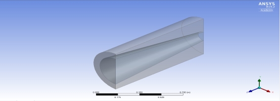
An axisymmetric half-cylindrical geometry is designed for the boundary of the simulation. The geometry has the diameter,

Dof 0.4 m and the length,

Lof 1 m. According to the theory of round jet (Kundu and Cohen, 2008), the diameter of the outlet,

doutletof the jet having the inlet with the diameter,

dinletof 0.12 m is obtained by using the equation:

	doutlet=4R12	(3.1)

where

	R12=Lξ12U	(3.2)

Note that

ξ12Uis a constant for round jet with a value of 0.09. Therefore,

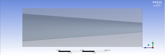
doutlethas a value of 3.6 m. The boundary was built in the form of:

L=1m

D=0.4m

doutlet=0.36m

dinlet=0.12m

Figure 3‑1 Side view of the boundary

Figure 3‑2 Isometric view of the boundary

The main reason for setting the boundary as illustrated as above is to saving mesh. The axisymmetric geometry of the allows the simulation calculate half of the turbulent jet which significantly save the mesh so saving the time of calculation. Considering the turbulent jet only behaves along the its propagation direction, the expansion of the jet is estimated based on round jet theory, which avoids the over-meshing in the part of air surrounded.

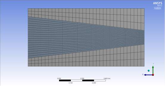In the mesh part, body sizing is used to mesh the boundaries of surrounding and jet. The element sizes are set to 0.03 m and 0.01 m for surrounding and jet respectively and other settings are kept default. There are overall 57,538 elements generated eventually. The side view of meshed boundary and boundary names are presented in Figure 3-3. The solver is set to density-based with absolute velocity formulation and steady time-step since compressible flow is expected for this simulation. Standard

k-ϵmodel is chosen with standard wall function and all the constants as default values. In the material selection, air is chosen to be computed using ideal gas law since compressible flow is considered. In the boundary condition section, surrounding inlet is set as velocity-inlet with no velocity vectors where surrounding outlet and jet outlet are set as pressure-outlet. Obviously, symmetry is set to type symmetry. Since the User-Defined velocity profile for jet inlet is still under development, an exhaust velocity of Mach 0.8 is used with initial gauge pressure of 2,000,000 Pa and outflow gauge pressure of 101,325 Pa for the jet inlet.

Surrounding outlet

Surrounding inlet

Jet inlet

Jet outlet

The symmetry is the flat side presented in the figure

Figure 3‑3 Side view of meshed boundary

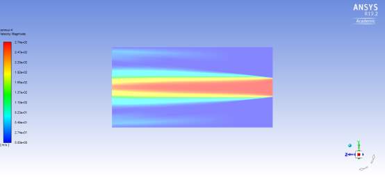
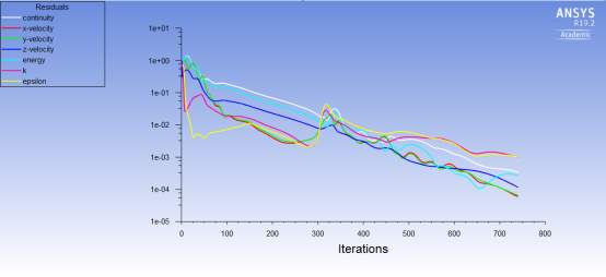For the solution method, the implicit scheme with default Courant number of 5 is chosen since the steady time-step is used. All the convergence criterions are set to 0.001. Standard Initialization is used to compute from jet inlet and the reference frame is chosen to be relative to Cell Zone. The results are presented below.

Figure 3‑4 Convergence of k-

ϵ

Figure 3‑5 Velocity Contour

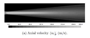The validation is conducted in terms of the behaviour of the jet. According to the research by Alessandro Bassetti (Bassetti, 2009, p. 130), the RANS solution from his research presented in figure 3-6 highly coincide the result in figure 3-5.

Figure 3‑6

3.2  Work to be done

The presented simulation is conducted in a small scaled model which does not match up with real scaled nozzles of aircraft engines, however, larger scale leads to large amount of calculation required. Still, a larger scaled model is considered to be used later. On the other hand, the simulation does not present a comprehensive behaviour of the turbulent jet due to the limited size of the boundary set in which further improvements will be conducted.

As mentioned in the previous section, User Defined Functions will be developed for the simulation performing better results. The solution methods need to be further selected for more stable iteration.

The rest two of

k-ϵmethods will be performed as soon as all the details in the standard one are suitably addressed. The noise propagation simulation will be conducted using FWH model based on these three

k-ϵsolutions.

4        Project Management

Figure 4‑1 The initial plan

ACTIVITY	PLAN START	PLAN DURATION	ACTUAL START	ACTUAL DURATION	PERCENT COMPLETE	Week
						1	2	3	4	5	6	7	8	9	10	11	12	13	14	15	16	17	18	19	20	21	22	23	24	25	26	27	28	29			Plan Duration
Literature Review	1	18	1	18	50%																																Actual Start
Initial Plan	1	2	1	2	100%																																% Complete
Model (standard)	3	3	4	3	100%																																Actual (beyond plan)
Mesh (standard)	3	3	4	3	100%																																% Complete (beyond plan)
Setting Up (standard)	3	3	4	3	100%																																Important Deadline
Simulation (standard)	3	3	4	3	100%																																Christmas
Project Proposal	7	2	8	1	100%
User-Defined Function	9	1			0%
RNG k-ε	10	2			0%
Realizable k-ε	12	1			0%
Noise Propagation	19	2			0%
Refinement & Validation	21	4			0%
Poster	20	2			0%
Presentation	23	1			0%
Final Report	23	7			0%
Initial Concept Report	1	5	4	2	100%
Final Concept Report	6	4	6	4	80%
PDR Report	10	3			0%
Trade Show	12	1			0%
AERO Lab	7	1	7	1	100%
AERO Quiz	8	2	8	2	100%
Exam Questions	6	3	6	3	100%
Thermal Lab	9	1			0%
CFD Report	4	2	4	2	100%
CFM Report	10	2			0%
Management Quiz	12	1			0%

*Note that the cells in blue are the individual project. The rest of the cells involve the plans for other modules.

5        References

Anselmet, F. and Mattei, P. O. (2016) Acoustics, Aeroacoustics and Vibrations, Acoustics, Aeroacoustics and Vibrations. doi: 10.1002/9781119178361.

ANSYS.Inc (2009) The Ffowcs Williams and Hawkings Model. Available at: http://www.afs.enea.it/project/neptunius/docs/fluent/html/th/node236.htm#eq:fw-h3 (Accessed: 14 November 2018).

Bassetti, A. (2009) A statistical jet-noise model based on the acoustic analogy and a RANS solution, Science.

Brentner, K. S. and Farassat, F. (1998) ‘Analytical Comparison of the Acoustic Analogy and Kirchhoff Formulation for Moving Surfaces’, AIAA Journal. doi: 10.2514/2.558.

Kundu, P. K. and Cohen, I. M. (2008) Fluid mechanics, Volume 10, Boston: McGraw-Hill Book Company. doi: 2001086884.

Launder, B. E. and Spalding, D. B. (1972) ‘Lectures in Mathematical Models of Turbulence’, Academic Press. doi: 10.1007/978-3-540-75759-7_75.

Lighthill, M. J. (1951) ‘On Sound Generated Aerodynamically. I. General Theory’, Society. doi: 10.1098/rspb.1979.0086.

Lighthill, M. J. (1954) ‘On Sound Generated Aerodynamically. II. Turbulence as a Source of Sound’, Proceedings of the Royal Society A: Mathematical, Physical and Engineering Sciences. doi: 10.1098/rspa.1954.0049.

LIGHTHILL, M. J. (1963) ‘Jet Noise’, AIAA Journal, 1(7), pp. 1507–1517. doi: 10.2514/3.1848.

Orszag, S. A., Yakhot, V., Flannery, W. S., Boysan, F., Choudhury, D., Maruzewski, J., & Patel, B. (1993) ‘Renormalization Group Modeling and Turbulence Simulations’, in Near-wall turbulent flows. doi: 10.1016/j.qref.2003.07.002.

Shih, T. H. et al. (1995) ‘A new k-ε{lunate} eddy viscosity model for high reynolds number turbulent flows’, Computers and Fluids. doi: 10.1016/0045-7930(94)00032-T.

Tam, C. K. W. (1998) ‘Jet noise: Since 1952’, Theoretical and Computational Fluid Dynamics, 10(1–4), pp. 393–405. doi: 10.1007/s001620050072.

Tucker, P. G. (2008) Unsteady Computational Fluid Dynamics in Aeronautics, Springer.

Williams, J. E. F. (1963) ‘The Noise from Turbulence Convected at High Speed’, Philosophical Transactions of the Royal Society A: Mathematical, Physical and Engineering Sciences. doi: 10.1098/rsta.1963.0010.

---

This dissertation proposal has been written by a student and is published as an example. See our guide on How to Write a Dissertation Proposal for guidance on writing your own proposal.