CFD Modelling and Analysis of Air Flow Around Lorry
Info: 14996 words (60 pages) Dissertation
Published: 16th Dec 2019
Tagged: Engineering
Content
Current study of Current Aerodynamics Reduction of Typical Lorry
Comment on variable convergence
Flow patterns analysis-Side View
Flow patterns analysis-Top View
Comparison of Different Driving Condition
Comparison of different Modifications of Geometry
Project Description
The aim of this project is to study the air flow pattern around lorry and to develop a CFD model to improve understanding of the flow and to develop more streamlined flow.
Summary
Nomenclature
A Lorry frontal area [m2]
Cd Drag coefficient [−]
∆Cd Difference in drag between the specific case and the reference [−]
ρ Density [kg/m3]
F Drag force [N]
FR roll Rolling resistance [N]
V Velocity [m/s]
T Time [s]
P Pressure [Pa]
µ Viscosity [kg/m · s]
g Gravity in [m/s^2]
p Specific heat capacity [J/kg · K]
T Temperature [C°]
Y plus (Y+) Dimensionless wall distance [−]
Abbreviations
CFD Computational Fluid Dynamics
CAD Computer Aided Design
DC Drag Counts
DNS Direct Numerical Simulation
LES Large Eddy Simulation
RANS Reynolds Averaged Navier-Stoke
Introduction
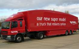
Today one of the most important issue for automotive industry is to reduce the emission and cost of running fees since the global fuel price continue to increase day by day. Especially for the heavy commercial vehicles and the heavy lorry is known for extremely inefficient compared with other ground vehicles partly because of its high aero drag and streamlined body. Heavy commercial lorry consumes approximately 52% of total fuel to produce the power required to overcome the aerodynamics drag when it is travelling at speed around 100Km/h [1]. It is researched that a typical lorry travels around 130000 and 160000 miles in the US each year [2]. Thus, reducing the aerodynamic drag of lorry can significantly reduce the fuel consumption each year. What is more, some of European countries like UK have decided to realise a more restrict law to reduce the car emission especially the heavy lorry (>10 tons) and increase the efficiency of utilising the fuels better. Despite various investments have been done over the decades, there are still a lot of the aerodynamics improvements that can be invested today. It is found that various mechanical add-ons like the sealed-gap and teardrop on the trailer, can be inserted to a typical lorry in order to decrease the pressure difference between head of the tractor and rear of the trailer and to reduce the formation of the vortex which will waste a lot of the energy. Most of these add-ons do not influence the front project area but do improve the streamlined aerodynamic of the lorry. Thus, better aerodynamic performance brings better fuel consumption and emission as well.
In the previous study it shows that even save the fuel consumption as little as 1% will save as much as 30 million U.S dollars each year. In 2009, it is found that 1.3 trillion petrels and diesel are consumed by the road vehiclesand as a result thousands of tons the pollution of CO and CO2 emission [2].
Although new designs of efficient lorry are designed every year in some brands like Volvo and Man manufacture, there are only a few studies and investment on the aerodynamic improvement for the current lorry on the road. Considering of huge amount of conventional lorry in use today, it is still essential to investigate the aero-drag reduction of the traditional lorry through lorry add-ons.
In other words, companies and manufactures who can build a lorry with welled-designed aerodynamic shape which saves more fuels can obvious be more competitive in the world market. Thus, designing a more efficient lorry is essential in the current stage.
In this report, a 1:4 scale typical heavy lorry is investigated. The reason for choosing this scale is that full scale lorry (around 16 meters lorry) will produce more than 10 million meshes in order to get reasonable results. Besides, due to current limited computer resource in use in university computer Centre, a full scale lorry is beyond the computer capacity. In this simulation, first of all, the flow patterns around a typical heavy lorry will be studied through the commercial CFD software- ANSYS-Fluent. Then, 3 add-ons (Sealed-gap, frame Extension, aero Teardrop of lorry) will be investigated in order to produce more streamlined flow and to see if the aerodynamic performance of lorry is improved and how much is improved.
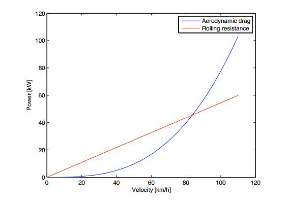
Figure 1: Power VS Velocity
Figure 1 shows the power required to overcome aerodynamic drag and rolling drag as a function of speed for a heavy commercial lorry. It is clearly that below velocity of 80 Km/h the rolling drag is greater than aerodynamic drag. However, after the velocity increases the aerodynamic drag increases dramatically and is much higher than the rolling resistance. This means that at high speed especially when the lorry is travelling a long distance, the aerodynamic drag becomes dominated. Thus, by reducing the aerodynamic drag the power required to overcome aero drag would be reduced.
Literature review
Background of CFD
CFD (Computational Fluid Dynamics) is a subject of fluid mechanics which uses mathematical method and numerical analysis to investigate the flow situations. Since the development of computer technology, most fluid problems can be solved in a reasonable error using the computer with certain CFD software. Especially for some of supercomputers, better results can be achieved. Wind tunnel was the only way to simulate flow problems decades ago, but with the help of Computational Fluid Dynamics and development of high performance computers CFD simulation can be applied to the fluid problems as well as wind tunnel experiment.
The governing equation of CFD problems is Navier-Stokes equations which governs many single-phase fluid flows. In order to make this equation simplifier, some parts in this equation can be removed like terms describing viscosity and vorticity. For cases like subsonic and supersonic flow, these equations can be linearized. For cases in transonic and hypersonic problems, equations can be modified in another ways.
Some years ago, methods are firstly used in order to solve linearized potential equations. After that, two-dimensional (2D) methods were developed in the 1930s by means of cases of air flows around a cylinder and aerofoil [3]. Lewis Fry Richardson did the first modern CFD calculation by means of divided the physical space into some cells using finite difference [4]. Although this exam failed at last, this method became the basis of modern CFD methodology. 3D simulation was also developed with the increase of computer power. After that the first paper of 3D model was published by John Hess in 1967. Programming of CFD developed a lot during that time and quantities of CFD codes including 2D and 3D were developed like (CFL3D, OVERFLOW developed by NASA) based on the Navier-Stokes equations.
Procedure of CFD analysis
As the commercial codes in CFD developed so well in modern society, today’s users of CFD are required to know much different knowledge compared with yesterday’s CFD users. It is not always necessary for today’s CFD users to program or design a series of Codes when doing the CFD. There are many advantages of these commercial CFD codes. For example, for those who never learn CFD basic theory can still finish some basic operations like sketching the geometry of the domain, setting up some physical parameters and applying the numerical methods to solve the fluid problems. Credits should be given to these development of CFD codes. Generally speaking, a normal CFD analysis consists 3 elements:
- Pre-processing
- Solver
- Post-processing
Pre-processing
The first step is using the Computer Aided Design (CAD) to sketch a geometry of the problem which can be in both 2D and 3D sketch based on the necessity of certain problems.
The second step, which is one of the most important steps, is the mesh generation. The geometry volume can be divided into some smaller subdomains or so-called discrete cells so that the flow physical property can be solved through each single subdomain. For example, in 2D cases, the mesh can be divided using uniform or non-uniform structure such as triangle or rectangular. Similar in 3D cases, volume domain can be divided by tetrahedral, Hexahedral and prismatic elements. One factor needed to be considered is that the accuracy of CFD problem is strongly influenced by the number of meshing cells and the quality of cells. Thus, gaining essential experience of how to design a good mesh is very important to a CFD user/ engineer.
After the meshing part is finished the next step is to select the physical and fluid property. A CFD engineer must correctly set up the fluid property so that the fluid characteristics of the fluid can be simulated accurately. For example, air and water have different fluid property like density and viscosity and these properties will be assigned to certain fluid cases. Only if the engineers set up these properties correctly can the Solver simulate the reasonable results. All the properties can be imposed through GUIs in the CFD commercial software like ANSYS-Fluent.
Boundary conditions is one of the most important part in CFD analysis and is required to consider after property setting up. Thus, whether or not the boundary condition is understood correctly and applied correctly to certain problems by the CFD users strongly influence the CFD Solver results. Also, if the boundary condition is not applied correctly the calculating time for the computer may be more than those situation that a good BCs are applied. In the transient fluid problems, not only the basic boundary conditions need to be considered but the initial values have to be considered as well.
Solver
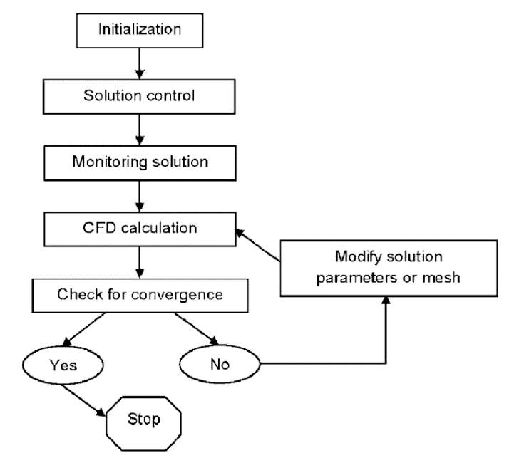
As mentioned above, each CFD problem can be divided by countless subdomains which represent a single PDE equation. These subdomains are in the form meshes and solver is, by its meaning, to solve these accountable Partial Differential Equations in terms of Mass Conservation Equation, Momentum Equation and Energy Equation. Nowadays, some commercial Solver codes are developed by companies like ANSYS Fluent, STARCD and OPENFOAM, etc. These codes become an efficient tool for the CFD user to solve the CFD equations through which users can choose different solve algorithms like Simple, SimpleC, etc. Generally speaking, a standard process of CFD solver can be concluded as initialization, solution control, monitoring solution, data calculation and check of convergence.
The graph below can describe how the solver works [5]:
 Post-processing
Commercial CFD codes like ANSYS-Fluent, developed the vivid graphic function very well in the post-processing. These outputs are promotional and visual, which make it possible for the users to see the results and process directly. In this process, most of the results could be got from the post-processing. The typical forms of CFD-post processing are: X-Y plots, Vector plots, Contour plots and other plots like streamline and animations. Not only can post-processing provide the visual contours to the users, but it can report data and output that users are interested in.
Figure 2: CFD procedure
All in all, a complete CFD analysis includes Pre-processing, Solver, and Post-processing stages. This procedure allows the users get a reasonable analysis results as long as they follow a correct step and set up all parameters correct. With the development of CFD commercial codes, simulations become more convenient than ever before. But, CFD simulation is still driven by a “Black-Box” which is under the control of raw CFD codes and most of the CFD users are not possible to get in touch of these raw codes.
Basic Theory of CFD
2 most famous methods of discretization are FVM (Finite Volume Method) and FEM (Finite Element Method)
FVM (Finite Volume Method)
The finite Volume method is a common approach used in CFD codes which is better than some other methods in terms of saving memory usage and solution speed especially in some large problem or turbulent flow with high Reynold number or situation like combustion.
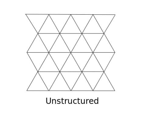 Finite element is the small volume surrounding each node referring to a mesh. In this FVM method, integrals of volume through partial differential equation (PDE) which has a convergence part are converted to surface integrals by means of the divergence theorem. These parts are measured as fluxes on the surface of every element volume. This method is conservative, because it is identical to that leaving the adjacent volume of the flux entering a certain volume. The FVM has many advantages, for example, it is easily to formulate to allow both structures and especially for unstructured meshes. In this way, the finite volume method is therefore suitable for some complicated meshes and complex
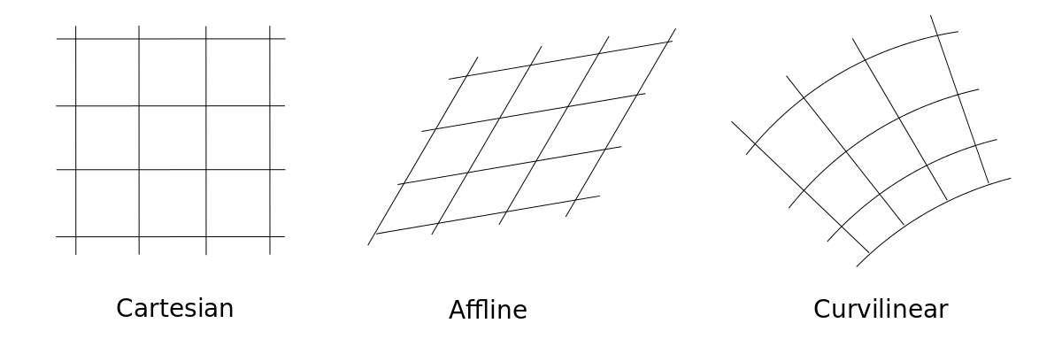
geometry.
Figure 3: 2D Structured Grid examples
FEM (Finite Element Method)
FEM (Finite Element Method) is a numerical method for solving mathematical and engineering problems which is usually applied in the structure solid problems, but due to its advantage of good calculation accuracy it is applied to the N-S equations and is used in the Fluid problems as well. One the advantages of FEM is more stable in the iterations than FVM. But FEM need much more computer memory and running time than FVM method. A weighted residual equation is applied in this method:
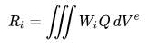
(Where the R is Residual, Q is the conservation equation, and W is the weighted factor, and V is the Volume of this Element)
Governing Equation
Naiver-Stokes Equations
In the Computational Fluid Dynamics, the Naiver-Stokes equation is the most important equation describing how the viscous fluid substances moves in the domain. It is useful because some fluid phenomenon which people interested in can be described in this equation. Continuity Equation, Momentum equation and energy equation are the key components in the Navier-Stokes Equations. Generally speaking, the N-S equations are based on Mass Conservation, Momentum Conservation and Energy Conservation. All the N-S equations are from these 3 conservation rules.
The N-S equations have a continuity equation of Mass Conservation which is depended by the time variable (t), 3 momentum equations depended by the time variable and 1 energy equation from energy conservation. There are 4 independent variables in these equations which are X, Y and Z components as well as t (time) variables. 6 dependent variables are in these equations as well. They are u, v and w vector components in the direction of X, Y and Z separately and density (rho), pressure (P) and Temperature (T) in the Fluid domain. All these dependent-variables are of functions to the 4 independent variables which can be expressed in a form of PDE equations below:
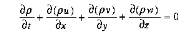 Continuity:
(Mass Conservation)
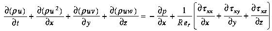
X-Momentum:
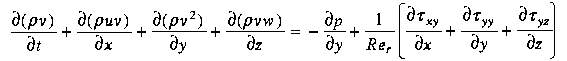
Y-Momentum:
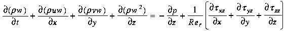
Z-Momentum:
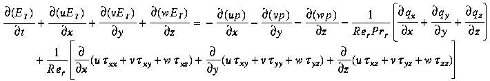
Energy:
The governing Equation for compressible flow in Cartesian coordinate
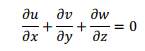
Mass Conservation:
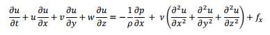
X-Momentum:
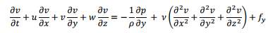
Y-Momentum:
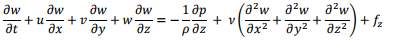
Z-Momentum:
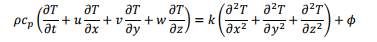
Energy:
The governing Equation for incompressible flow in Cartesian coordinates
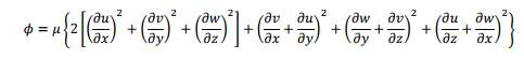 The dissipation function of the energy function is given by:
These equations above are of 3-Dimensional unsteady form of N-S equation and they are derived by George Gabriel Stokes and Claude Louis Navier in the year 1800 in the England and France. These equations describe the relationships between the temperature, velocity and density of a fluid. These equations are very complex thus at current stage of undergraduate only basic forms of Continuity, Momentum and Energy equations are described. Those equations with fully derivation will not be considered in this report because it is more essential to discuss the application of CFD rather than a fully theory of CFD. These equations are a series of Coupled PDE (Partial Differential Equation) and could be applied to the physical Fluid problems by means of different methods of mathematics. However, these PDE s are so hard to solve analytically that scientists in the past had to do some simplification and essential modification to these equations in order to solve these equations. Recently, the calculation of these equations become easier than situations many years ago due to the help of Finite element analysis methods mentioned above and development of high performance computer.
Current study of Current Aerodynamics Reduction of Typical Lorry
Truck aerodynamics
Usually the aerodynamics force of ground vehicles includes 2 types: pressure drag and friction drag. The pressure drag is the force acted perpendicular to the driving direction due to the pressure difference between head and rear part of the lorry while friction drag is formatted due to the shear stress between the surface of lorry and air. For a typical commercial lorry, the pressure difference head of tractor and rear of trailer can be vast, which causes a significant pressure drag. As R.M. Wood said in his book Impact of “advanced aerodynamic technology on transportation energy consumption [5]”: nearly 90% of the drag is made of pressure drag. Form some literature finding, it is possible to say that shape of tractor, gap between the trailer and tractor can be the dominant drag factor, as well as the complex geometry of trailer base.
Major Modification Considered
1-Deflector
Although most of the modern typical commercial Lorries are well designed, some conventional Lorries which is lack of aerodynamics consideration are still in use now. One typical problem in aerodynamics of traditional lorry is huge flow separation at upper corner part of the tractor. This separtion of flow will increase the pressure difference at this region and therefore reduce the streamlines of flow around tractor.
Without Deflector
With Deflector
Figure 4 a: Without Deflector
Figure 4 b: With Deflector
2-Tractor-trailer gap
 The gap between the tractor and trailer is a significant factor influencing the Drag. When the lorry is moving at a speed, the air hits the trailer front and then goes into the gap, which will format a pressure drag. If the height difference between the tractor and trailer is great, the pressure drag will be greater as well. The pressure drag will increase dramatically especially when cross wind situation appears. There are some common add-ons used to lead the air through gap space. The first one is, as mentioned above, the deflector is one of the best ways to avoid huge flow separation. Another way to improve aerodynamics is adding a side deflector especially for huge gap. The main purpose for these add-ons is to prevent the un-controlled circulation in the gap and cross flow as well. Both flow types will harm aerodynamic performance during the driving condition.
Gap Treatment
Figure 4 c: Gap treatment
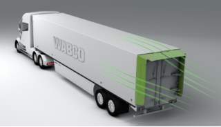
3-Undercarriage and Aerodynamics trailer
Because of a lot of irregular geometries with shape edges existed on the surface under the tractor and trailer, some unexpected turbulent flow is therefore formatted under the lorry. These turbulent floe will reduce the streamlined flow under lorry and at the same time increase both pressure drag and skin friction drag. With the rotation of the wheels, flow separations become more complex. As a result of these effects, some energy will loss while driving at high speed. In order to reduce these negative influence on the lorry drag, some different types of devices are designed such as Side Skirts and Bogey Wheel fairing. All these devices are to make the bottom of lorry as smooth as possible and reduce the side-effect of the rotating wheels.
Another method to make flow around trailer more streamed is a devices called aerodynamics Teardrop. This is a modification of the shape of top surface of trailer. A conventional trailer surface is a flat surface which will leads to the formation of base wake and huge flow separation in the region near the front trailer edge. However, after this aerodynamics teardrop is applied to the lorry, more streamlined flow passing through the trailer is produced and therefore reduce the pressure drag as well as the total drag of the aerodynamics drag.
Conventional Trailer
Teardrop
Figure 4 d: With Teardrop
Figure 4 e: Original lorry
4-Rear of the trailer
When the lorry is driving, the air flow passes through both top trailer surface and side surface and then these flows which are of low momentum meet at the rear trailer part. The interaction of these flows will generate a significant wake or called as Vortex, resulting an uncertain turbulent flow in the end of the trailer. As a result of these components, a low pressure region is formed which results in a big pressure difference and pressure drag. The normal devices to reduce the formation of these vortex and wake are Frame Extension, Base plate and Boat tail, etc. By leading the air flow along the Frame Extension, the flow separation could be decreased and strength of Vortex as well.
Frame Extension
Figure 4 f: With Frame Extension
Methodology
As mentioned before, this report focus on studying the aerodynamics performance of the flow around a typical heavy commercial lorry. The preferred commercial CFD software is ANSYS-FLUENT. In fact, there are several commercial CFD analysis software for use right now such as ANSA, STARCCM+ and CFX. But in this case, ANSYS-FLUENT is used to investigate the flow patterns and measure the aerodynamics factors like Drag coefficient, Lift coefficient and so on. In this case, the Solidworks is utilised to sketch a 3D model of a typical commercial lorry.
In this case, the original plan is to choose a typical 3D lorry model of Volvo-company. Unfortunately, due to the security reason of Volvo Company, the author is not allowed to use a real Volvo Lorry. In order to achieve an accurate geometry of a typical lorry, a 3D lorry [7] form a commercial website called GrabCAD is used. This 3D model not only provides all features of a real lorry but it is of 1:1 Scale to a real heavy size as well. Thus, it is possible to say that this lorry model can represent a typical commercial heavy lorry which is in used now.
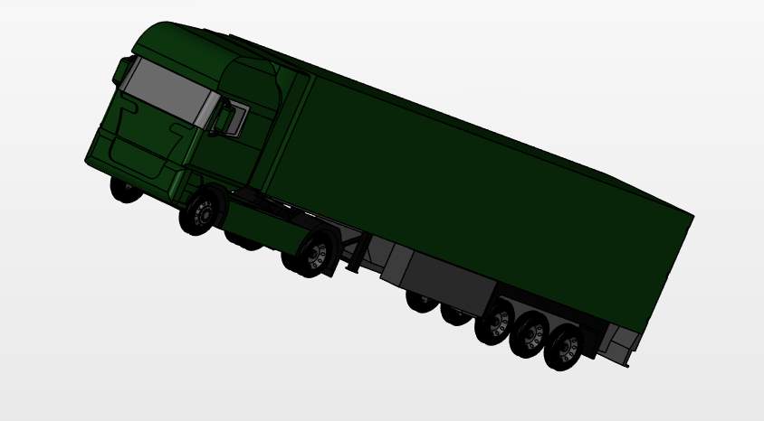
Figure 5: Lorry Geometry
Geometry
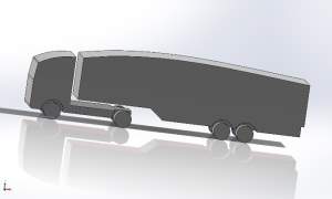
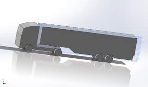
Although this 3D lorry form GrabCAD have similar features of a real commercial heavy lorry, it is not recommended to apply this 3D lorry into FLUENT for analysis. Instead, a new simplified 3D lorry of 1:4 Scale with similar basic dimensions of the real lorry model is sketched in Solidworks. The new sketched lorry model has basic geometry of real lorry. But some complex geometry which does not influence much of the flow patterns such doors is neglected. Similarly, some complex parts like bottom of tractor and trailer is too complex to analysis. Besides, it is not necessary to spend a lot of time and resource in doing analysis of this part in the current case.
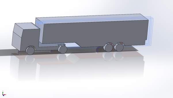
There are some reasons of doing a 1:4 smaller Scale simplified geometry. The first reason is due to the limited computing resource used for students. Generally speaking, the more complex the geometry is, the more difficult to generate a proper mesh for this lorry and more difficult for the FLUENT to converge even if a proper Turbulent Model is utilised. For example, in this case, the bottom of both tractor and trailer is so complex that it would take *5 times more computing resource than simplified model. The second reason is this lab focus on studying the main flow pattern around typical lorry and measuring the drag on the lorry, rather than investigating details of flow at some typical complex geometry. The simplified lorry geometry still keeps the main geometry but reduced some complex geometry which can be ignored for the purpose of this lab, so it would not change the major flow types around the lorry but decreased the meshing difficulty and increased computing efficiency at the same time. The last reason is due to mesh quantity of a full-size lorry. A full-Scale size lorry (about 16 meters long, 4 meters high, 3 meters wide) can generate over 10 million meshes even for this simplified lorry model which is not affordable in this case for student. Instead, a 1:4 Scale model is generated in order to decrease the cell numbers.
Figure 5a: Original Lorry Geometry
This picture above is the sketched 1:4 typical commercial lorry.
In this report, not only the original lorry is investigated, but Lorries with modifications which provide better aerodynamic performance are required to be tested as well. As mentioned above, there are several devises can be added to a lorry in order to produce more streamlined flow around the lorry. However, due to the limitation of both time and computing resource, this report focus on only 3 devices of add-ons.
- Lorry with Deflector
- Lorry with Deflector + Aero Teardrop
Lorry with Deflector + Aero Teardrop + Frame Extension + Vortex GeneratorFigure 5b-2)
Figure 5b-1)
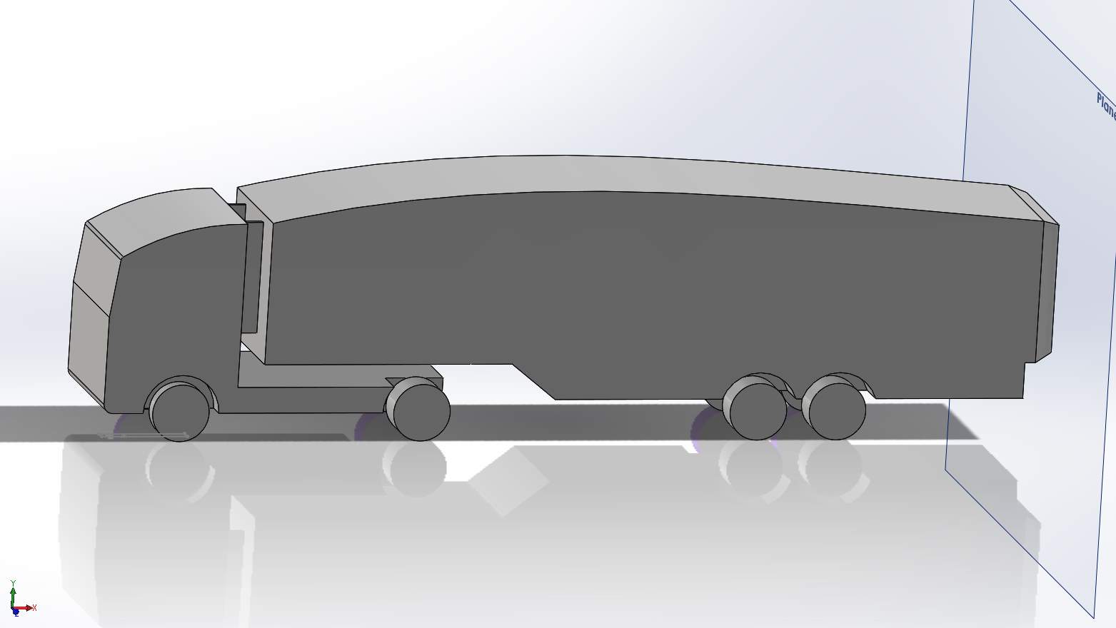
Figure 5b-3)
Reynold number Evaluation
Reality case analysis (V=25m/s, 15 C degrees, ISA situation):
The equation of Reynold number is:
Thus:
Re=ρ*V*Lμ
Re=1.225*25*160.0000181
=27,000,000
1/4th Scaled Model (V=25m/s, 15 C degrees, ISA situation):
The equation of Reynold number is:
Re=1.225*100*40.0000181
=27,000,000
From this equation, when characteristic length (L) become ¼th smaller than the original Length (16m), the Flow Velocity should be 4 times bigger than original speed (25m/s) which is 100m/s in order to have equal Reynold Number. It is agreed that the ¼th smaller scale modelwould produce the similar flow feature [8] if the Velocity is increased to 4 times bigger which will give the same Reynold Number.
In the case of flow around a free body such as a plate, Reynold number smaller than 2000 is considered as laminar flow, Reynold number between 2000 and 500,000 is in transition state and above b can be deemed as fully turbulent flow. The Reynold number for this case is around b, which is fully turbulent flow. Even the flow speed of 100m/s is high in this case, the air compressibility can still be ignored when velocity is smaller than Mach 0.3 (110 m/s in equivalent) at ISA situation.
Volume Mesh
At the beginning of this simulation, a 2D geometry is selected to simulate the air flow patterns around a lorry. However, 2D geometry is lack of many geometry details of a typical lorry, which will significantly influence the final simulation results. In order to improve the simulation accuracy, a 3D geometry is applied as well as 3D meshing.
Air flow Domain
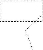
The dimension of the computational domain should be at least 3 lorry length in front of the lorry, and 5 times lengths behind. In terms of the domain next to the lorry, it should be at least 3 times wider than lorry width [9]. This domain could cover all features near the lorry surface.
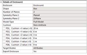
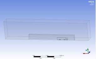
Since the lorry is in symmetric in left-right direction, it is possible to create a symmetric domain which is of half of the lorry geometry. This way it can decrease the computing resource and increase the efficiency of simulation.
Figure 6b: Enclosure dimensions
Figure 6a: Air Domain of original Lorry
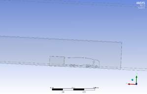
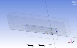
Figure 6d: Lorry with Deflector
Figure 6c: Lorry with all add-in
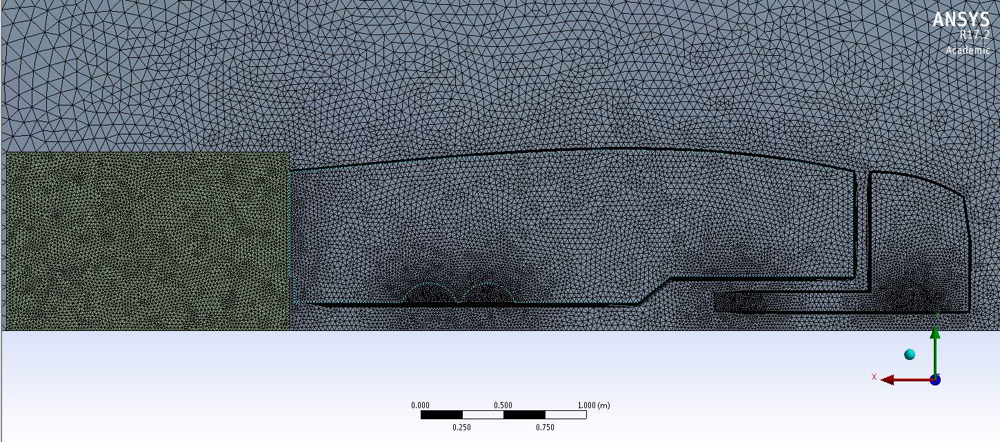
The meshing strategy is considered in this case. Generally speaking, there are 3 major methods to mesh the domain. They are adaption method, box method and control methods [8]. All three methods have their own advantages and disadvantages. In terms of this case, boxes meshing strategy is considered due to its high accuracy in some certain parts of the domain which users are interested in. in this domain, a hybrid mesh is created in order to decrease the total elements number whilst sketch accurately the complex shape of lorry. In the external domain, an element type of Hexahedron is applied which is easy to calculate and can decrease the amount of the cells. In the internal domain close to the lorry surface, a tetrahedron element type is applied due to its advantage of unstructured shape which can sketch complex geometries.
Near-wall Treatment
As mentioned above, situation of this case is fully turbulent flow which needs specific wall treatment in the CFD simulation. The Turbulent model chosen is K-e turbulent model with Realizable wall function treatment. The reason of choosing this combination will be mentioned in the Set up analysis below. Thus, it is necessary for this mesh to guarantee a reasonable Y + value between 30 and 150 with the combination of certain turbulent model and wall treatment mentioned above [9]. An inflation method is inserted around surface of the lorry to sketch a first layer thickness of 0.7 mm (only in the original case) which is estimated by online first layer thickness calculator with given velocity and fluid property. After first simulation is finished, the Y+ contour can be checked if it meets the requirement of estimation. If not, different first layer thickness could be tested until the y+ value meets the requirement.
For the mesh of other modified lorry such as: Original lorry at different driving speed, Lorry with deflector and lorry with Frame Extension, similar meshing skills are utilised.
This first layer thickness ensures the wall function works well at near-surface region.
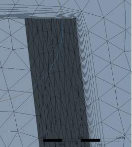
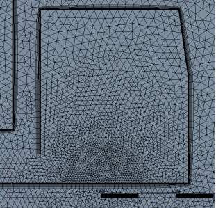
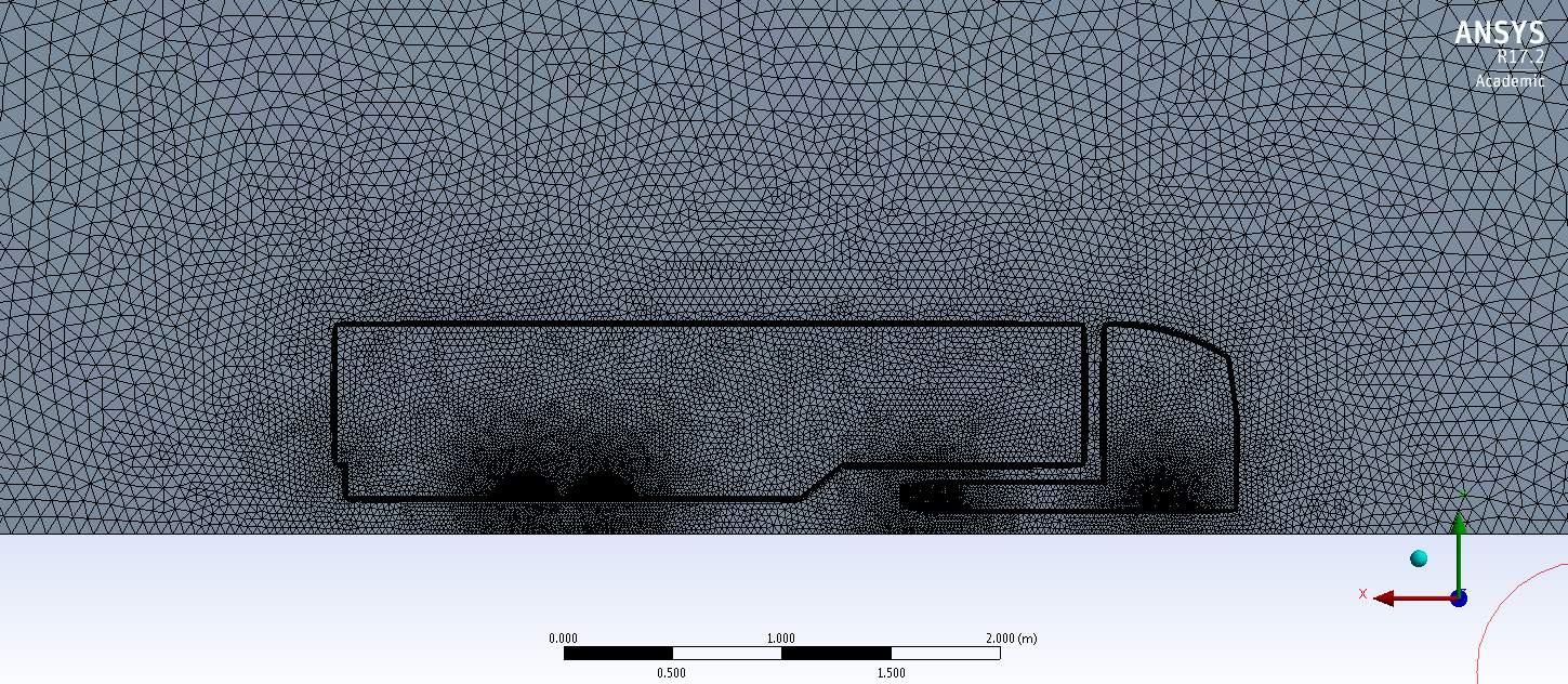
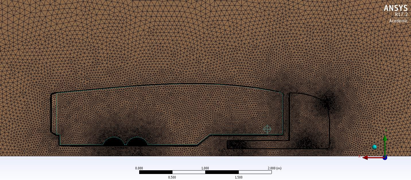
Figure 7a: Mesh
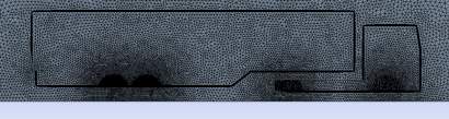
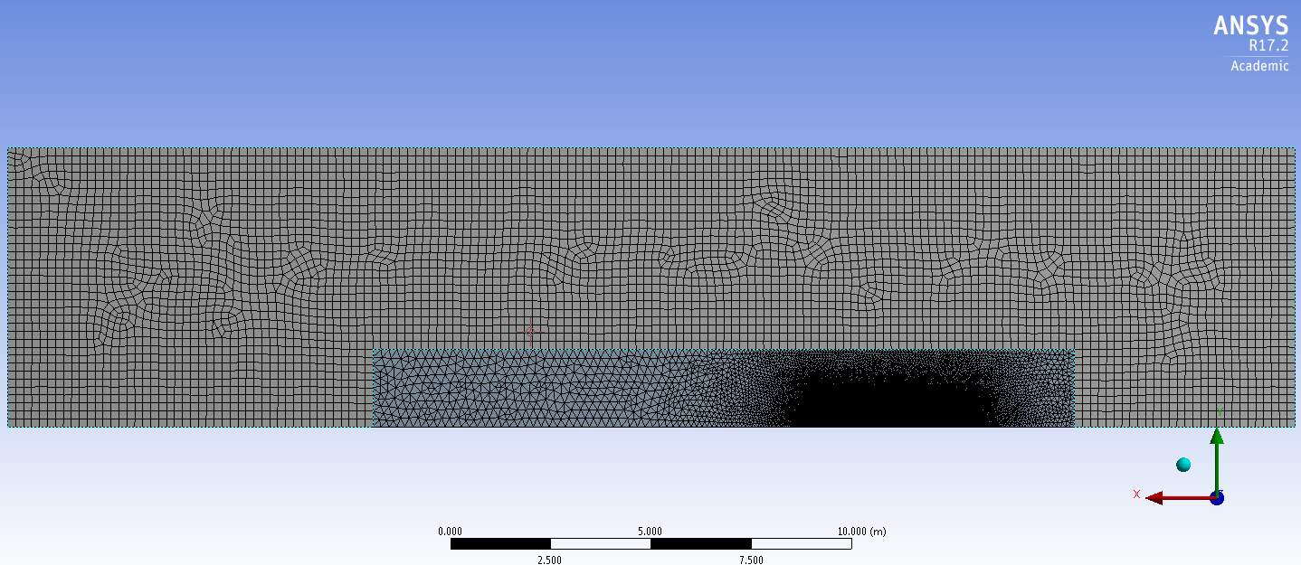
Figure 7b: Mesh of ORIGINAL Lorry
Deflector
Figure 7c: Mesh of Lorry with deflector
Deflector
Teardrop
Figure 7d: Mesh of Lorry with deflector +Teardrop
Teardrop
Frame Extension
Deflector
Figure 7e: Mesh of Lorry with All added-on
Physical models setting
Below is a brief description of the most essential models used for the simulation in the ANSYS-Fluent. Details of all Solver setting are in the Appendix B.
- Space type: 3D Model
- Motion: Stationary
- Time: Time–Averaged
- Material used: Fluid-Air (15 degrees, ISA)
- Equation of state: Constant density based
- Flow types:Turbulent flow
–Turbulence model: Reynolds Averaged Navier Stokes – K-e Realizable turbulent model.
–K-e Wall treatment: Non-Equilibrium Wall Function is utilised. This wall treatment can be used only when Y+ value meets the basic requirement between 30 and 200.
- Monitor setting: All variablesset to be below 10^-4
- Solver choice: SIMPLEC-First Order Upwind-(first 1000 iterations)-
Second Order Upwind-(following iterations in order to get more accurate results) Coupled with Second order upwind method (to get situation totally converged)
Brief comment of Strategy used in choosing turbulent model
The standard k-e model is widely used due to its good calculating efficiency and reasonable results. But this model performs poorly for complex flows involving severe pressure gradient, and huge separation. It is suitable for initial iterations and parametric studies.
The standard k-w has better performance for wall-bounded boundary layer, free shear, and some low Reynold number flows compared with k-e turbulent family. If the user is interested in studying the flow patterns in the boundary and separation region, the standard k-w would be the best option to choose. Unfortunately, using k-w model need a finer mesh whose first layer thickness or first cell height should be at y+=1 and a prism layer mesh with growth rate no bigger than 1.2 should be used[10]. In terms of this case, the Reynold number (27 million) determined is huge compared with the constraints of applying K-w model and it is impossible to draw a mesh with first cell height with y+=1 in this case due to the huge size of the geometry, high Reynold number, and the time, computing resource limitation.
Some any other models have their own advantages and disadvantages, it is not necessary to introduce all turbulent models in this report. All in all, considering the Reynold number, accuracy, computing resource available, and factors (Cd, flow patterns) this case is interested in, the standard k-e turbulent model would be the optimal model in this simulation.
Boundary Conditions
The goal of doing this project is to study air flow patterns around a typical lorry at different driving conditions and modify the geometry of lorry to produce more streamlined flow, which brings a lower drag Coefficient. Thus, simulations are divided by 5 parts as mentioned:
- Original case with 100m/s velocity
- Original case with 67m/s velocity
- Modified case with Deflector at 100m/s velocity
- Modified case with Deflector + Teardrop at 100m/s velocity
- Modified case with deflector +Teardrop + Frame Extension at 100m/s velocity
Therefore, there are 5 sets of Boundary conditions.
Case 1: Original Lorry with 100m/s
| Inlet | Velocity-Inlet | 100m/s |
| Outlet | Pressure-outlet | Gauge pressure (0 pa) |
| Top Domain | Symmetry | – |
| Side domain | Symmetry | – |
| Road | Moving Wall | 100m/s |
| Lorry surface | Wall | – |
| Interior domain | Fluid | Air (ISA) |
In the case of Original lorry with 67m/s, the moving road speed is modified to 67m/s and the rest of settings are kept the same.
In the case of modified cases, all boundary conditions are kept the same to the BCs above.
Simulations
The simulation is performed in the ANSYS–FLUENT. Each simulation run for 1000 iterations first in SIMPLEC method with First Order Upwind and another 3000 iterations with Second Order Upwind to get a more accurate result. After these setting, the original case converges at last meet the setting criteria of 10^-4. However, in the rest 3 modified cases, more complex flow is produced by some additional added-ons. The previous setting does not make the result totally converge. To solve this phenomenon brought by huge flow separation, another 500 iterations are performed using Coupled method to make the results totally converge.
In all the cases Residual plots at last reached the criteria of 10^-4 and all variables such as Drag coefficient (Cd) and Lift coefficient (Cl) this project is interested in reached convergence as well.
Result analysis
Grid Independence Analysis
Theoretically, the finer the mesh is the more accurate the results will be. However, due to the limitation of computing resource, it is impossible to calculate extremely huge mesh size. Thus, finding a good mesh which could ensure enough accuracy of this project’s goal with minimum mesh size is needed to be studied. This process is called grid convergence analysis.
In this process, 3 different meshes of the original lorry are invested which are Coarse, Medium and Fine mesh. The refinement factor is in the table below:
| Domain | Nodes | Elements | Refinement Factor 11 |
| Air-Fine mesh | 1,193,353 | 5,492,094 | 1 |
| Domain | Nodes | Elements | Refinement Factor 12 |
| Air-Medium mesh | 813,736 | 3,564,345 | 1.241 |
| Domain | Nodes | Elements | Refinement Factor 13 |
| Air- Coarse mesh | 336,095 | 1,199,551 | 1.723 |
Table 1 –Amount of Elements
To better check the grid convergence in this case, two variables of Drag coefficient (Cd) and Lift coefficient (Cl) are chosen to detect if the mesh reached grid independence. A table of variant CD, Cl of 3 meshesis sketched with respect of 1/R (Refinement factor)
| Coarse | Medium | Fine | |
| 1/R | 0.347826087 | 0.628184 | 1 |
| Cd | 0.82038698 | 0.7961 | 0.802052 |
| Cl | -0.17952462 | -0.17062 | -0.16732 |
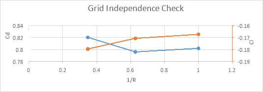
Table 2 –Cl, Cd at different meshes
Table 3– Grid Independence Check
From this graph, the difference of two different variables Cl and Cd between Fine mesh and medium mesh is much smaller than the difference between the difference between medium mesh and coarse mesh. It is possible to state that from these 2 variables the medium mesh can be deemed as grid independence, which means a finer mesh will not improve the result accuracy but waste some computing resource.
Another method to verify if this mesh is in grid independence is to compare the flow patterns among coarse, medium and fine mesh.
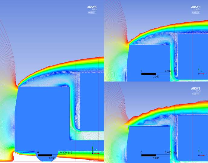

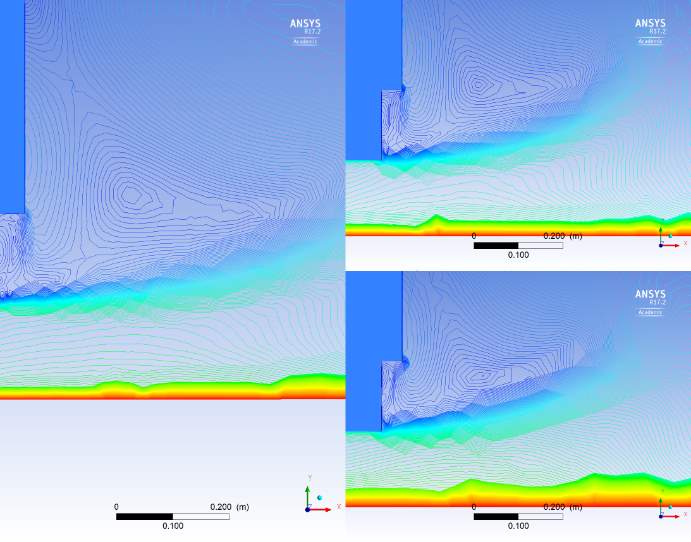
Fine mesh
Medium mesh
Coarse mesh
Figure 8: Flow pattern features of 3 meshes (Coarse, Medium, Fine Mesh)
In this contour of velocity at 3 different views, the flow types are all similar and distribution of flow types is similar as well. Taking closer look of both front and rear oart of this contour, it is clearly that flow distribution at fine mesh and medium mesh is nearly the same. So, there is no need to use a finer mesh simulating this case. The medium mesh can be deemed as grid independence as well from the perspective of checking flow patterns.
All in all, it is clearly that the medium mesh has reached grid independence. Therefore, the medium mesh with element amount of 3,564,345 is utilised in this project. This mesh is proved to be accurate enough and computing resource friendly. After doing this grid independence check, the flowing cases with geometry modifications will use similar mesh amount like this mesh.
Convergence Analysis
These graphs below are convergence history of Residual, Cl and Cd.
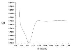
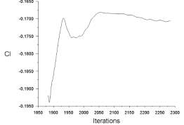
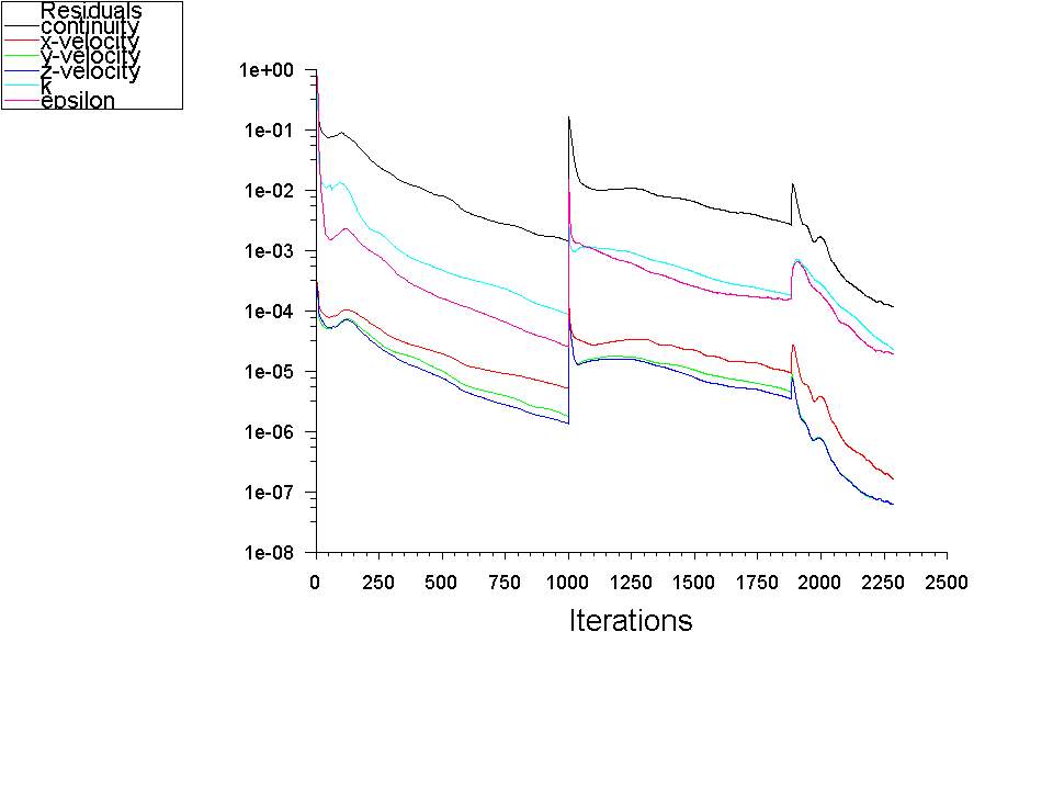
Figure 9—Original Lorry (100m/s) Residual, Cd, Cl convergence history
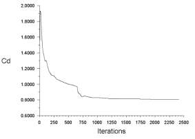
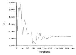
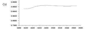
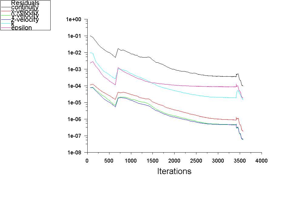
Figure 9a: Original Lorry (67m/s) Residual, Cd, Cl convergence history
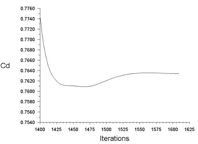
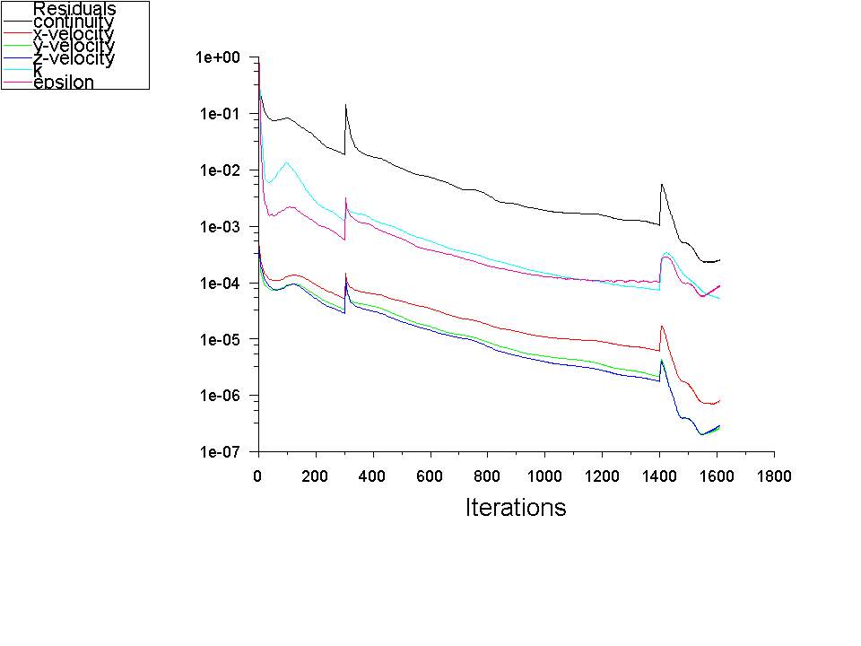
Figure 9b: Modified lorry with Deflector (100m/s) Residual, Cd convergence history
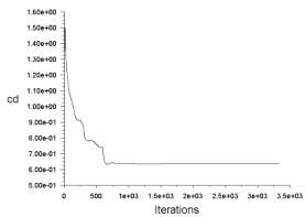
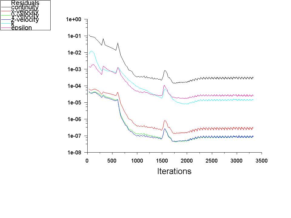
Figure 9c: Modified lorry with Deflector+ Teardrop (100m/s) Residual, Cd convergence history
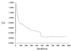
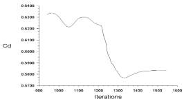
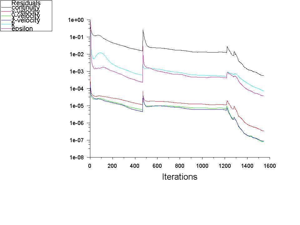
Figure 9d: Modified lorry with Deflector+ Teardrop+ Frame Extension (100m/s) Residual, Cd convergence history
Comment on variable convergence
These 5 convergence histories are about
- Original lorry in 100m/s
- Original lorry in 67m/s
- Modified lorry with deflector
- Modified lorry with deflector+ teardrop
- Modified lorry with deflector+ teardrop+ Frame extension
The number of iteration are set to be 10000 and the absolute criteria is set to be
10-4of residuals. In the case a), case b) and case c), all the variables go to below
10-4after 2250 iterations and Cd, Cl do not change any more. Although there is some ocilations around 4*
10-4of residual plot after 2000 interations in the case d), it is still possible to state that this case reached convergence as the Cd does not change any more after 2000 iterations. The rest cases all reached the convergence in both residual and Cd. The solver methods used in these cases are as follows: SIMPLEC- FIRST ORDER UPWIND (1000 ITERATIONS) –SECOND ORDER UPWIND (3000 iterations) – COUPLED (500 ITERATIONS)
The reason of using hybrid solver methods is because for some complex situation with complex flow separations it is difficult to get an accurate result in a short time with one solver method. The application of different Solver methods at different stages could reduce calculation time while improve calculation accuracy.
Y plus analysis
Y plus analysis is important in cases of fully turbulent flow. Y + is directly affected by the turbulent model chosen, wall function treatment applied and height of first layer thickness used. In this project, the reasonable Y plus range should be around 30 to 200 when k-e turbulent model, realizable wall function are applied.
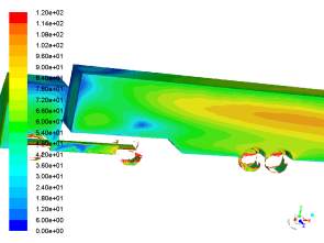
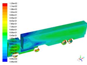
Figure 10b: Y plus of Original Case 67m/s
Figure 10a: Y plus of Original Case
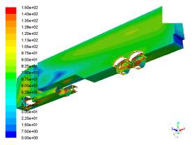
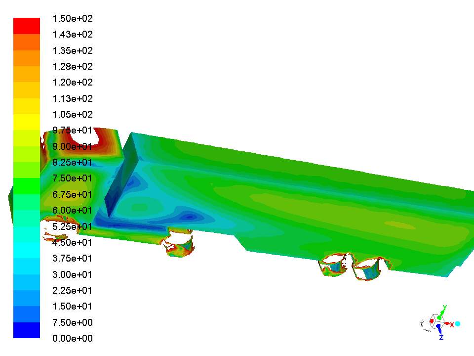
Figure 10 c: Y plus of Modified case (Deflector)
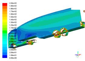
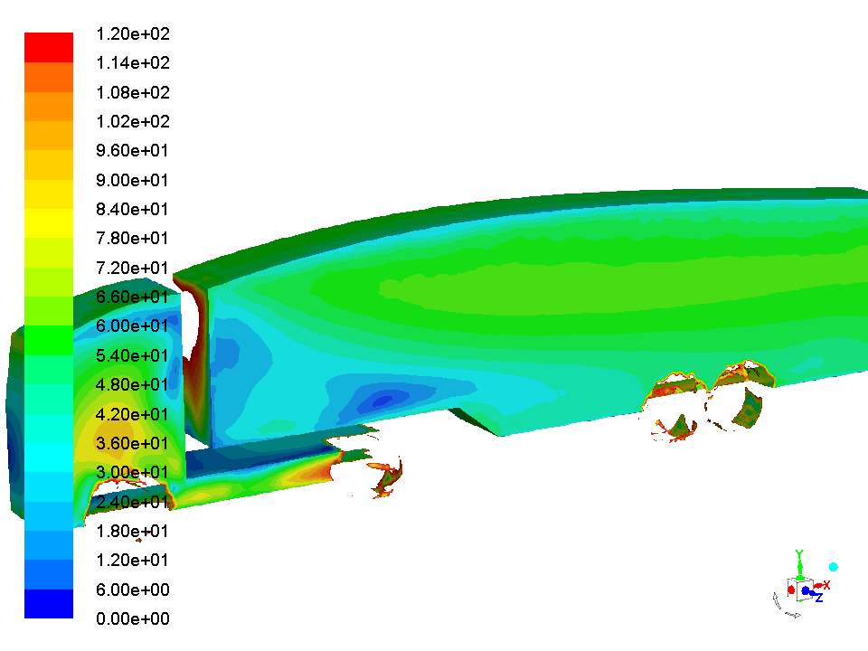
Figure 10d: Y plus of Modified case (Deflector +Teardrop)
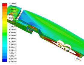

Figure 10e: Y plus of Modified case (Deflector +Teardrop +Frame Extension)
Comment of Y +
All situations have reached a good range of Y plus around 30 and 120 which is quite accurate to capture features near wall surface. Although a few place like wheel region has high Y+ value, it can be ignored when this feature does not affect final result people is interested in. This correct Y plus range ensures wall function work well which leads to good simulation results.
Flow Pattern Analysis
Flow patterns analysis-Side View


Upper Shear Layer
VC
VC
Lower Shear Layer
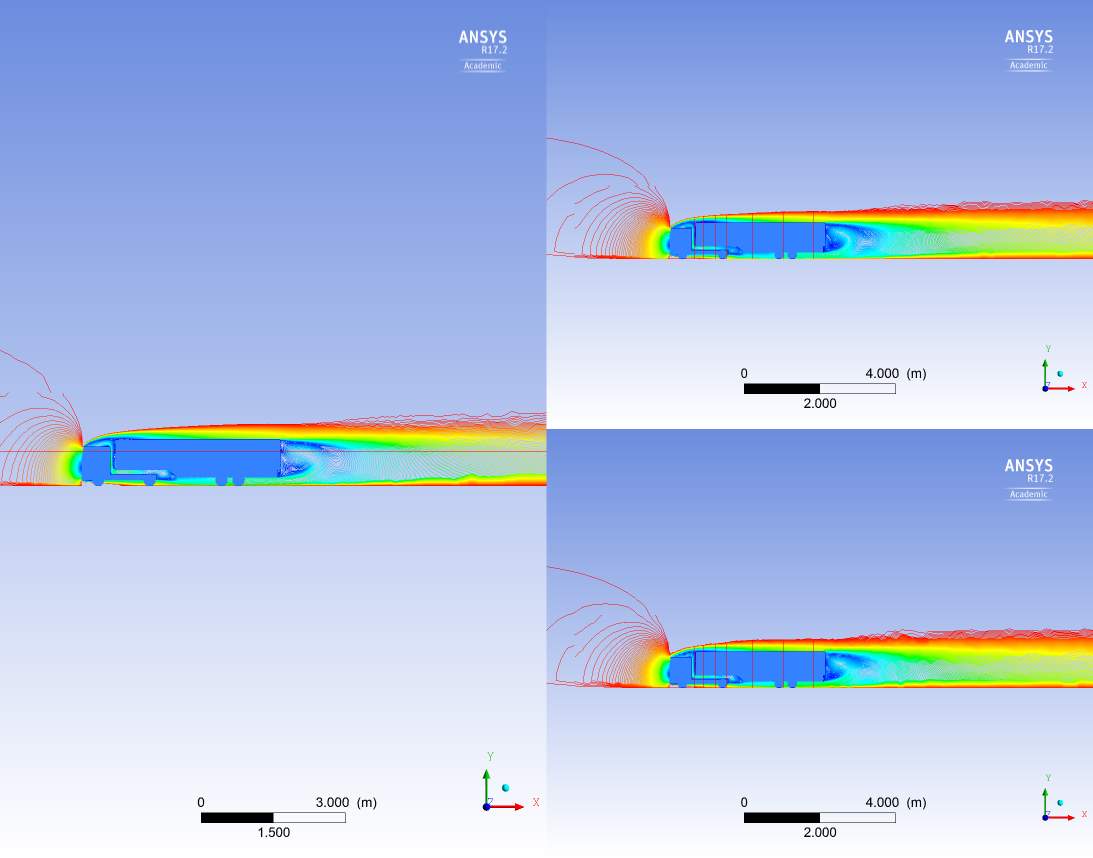
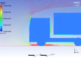
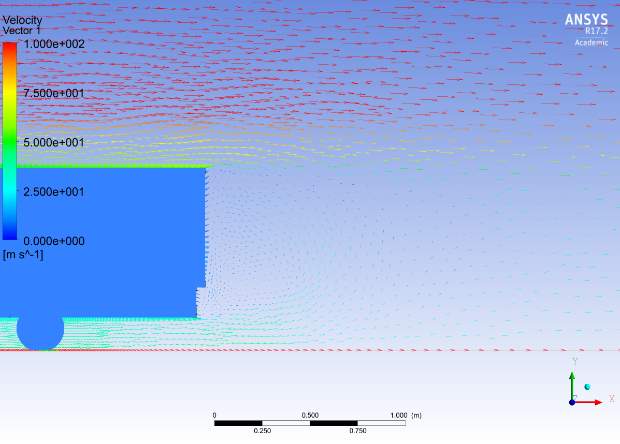
Figure 11a: Vector contour of Vector


SP

VC

ST
SP
Figure 11c
Figure 11b
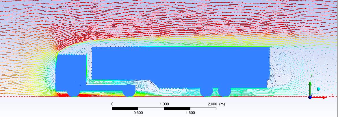
Figure a above shows the Vector contour of velocity of the original lorry in 100m/s. The upper contour presents a stream wise flow pattern over an original lorry. At the front of the lorry tractor the flow moves downwards and upwards around the tractor. A centre flow line separates the flow to upwards and downwards flow with its end called as the stagnation point (ST). At stagnation point the stream velocity is 0 and flow starts to separate at this point with acceleration along the curve surface of tractor. There is a huge flow separation happening at both upper and lower point of the front tractor face. Part of this flow goes into the gap region between the tractor and the trailer while the remaining flow continue flow around the surface of the trailer.
Figure b shows a closer look of the tractor geometry. A big flow eddy is formed at region above the tractor top surface. The stagnation point can be seen clearly as well as 2 big flow separations at upper and lower position of the tractor.
Figure c gives a closer look at rear part region. The formation of this vortex is clearly seen. At the rear part of the trailer, a massive flow separation is formed both on upper and lower surface which leads to the formation of both lower shear lower and upper shear layer. Because of the formation of both upper and lower shear layer, a huge vortex (VC) appears at the rear part of the trailer.
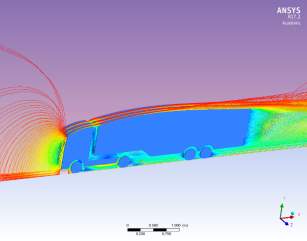
Flow patterns analysis-Top View


Flow separtion
SV
ST
Figure 11d: Vector Contour of Vector Spanwise-View
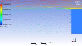
Figure d shows a velocity distribution contour when look at the lorry form the top view. The spanwise reference plane is captured at height of 0.5m in the 1:4 scale lorry. Before hitting the tractor face the air flows directly towards to the front of the tractor. The presence of the stagnation point makes the flow very hard to flow in its original direction, which means the incoming flow have to move around the tractor through the two sides. Since the geometry of tractor is in a blunt shape, this flow cannot follow the downstream flow of front tractor. Thus, this contributes to a massive flow pattern separation at the rear part of the tractor.
Figure 11e
At the rear part of the trailer, a spanwise vortices (SV) is formed. What happens in this region is that a low-pressure region is formed and the neighbouring region with high pressure moves into this low pressure region with flow rotations. The movements and the circulation of the flow at this region forms this result of a spanwise vortices (SV). As this is only half geometry of a typical lorry, theoretically there are 2 spanwise vortices at both left side and right side and the flow patterns at the other side should be the same. The strength of vortices is decided by the pressure difference and strength of flow circulation.
Comparison of Different Driving Condition
In this project, 2 different driving conditions are considered in reality which are at different driving velocity (90KM/s and 60KM/s in a full scaled lorry). However, in this practice, a 0.25 smaller scale model is applied which brings 4 times higher flow velocity to keep Reynold number the same. Thus, incoming flow velocity would be 100m/s and 67m/s in this case. The velocity contour is as below:
Figure 11g: Vector contour of Velocity
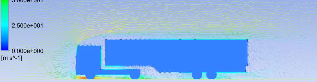
Figure 11h: Vector contour of Velocity
Figure g shows the vector distribution of 100 m/s case and figure h is the vector contour in 67 m/s case. The colour between these 2 contours is different because the range is set to 0 to 100m/s for both cases. Through the observation of two contours, the flow patterns are all similar except for the strength of vortex. The strength and area of vortex in 100m/s case is bigger than strength of 67m/s as well as spanwise vortices at rear part of the trailer.

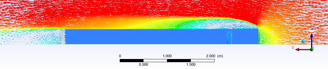
Figure 11i: Vector contour of Velocity
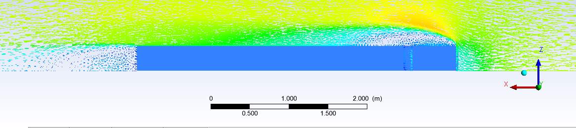
Figure 11j: Vector contour of Velocity
Figure I and figure j are vector contour viewing at spanwise direction. Not only the spanwise vortices at rear part of trailer differ between 2 situations, but the strength of flow separation at front tractor edge of 100m/s case is higher than 67 m/s case as well.

Through the Cd convergence history, drag coefficients in 2 cases are nearly the same despite they have different velocities. The error between them is 1.127% which is smaller than 5%. It can be deemed they have same Cd.
Comparison of different Modifications of Geometry
As mentioned above, the major modifications are Deflector, Aero Teardrop and frame extension.
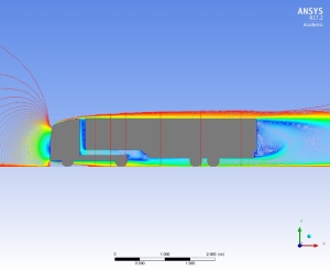
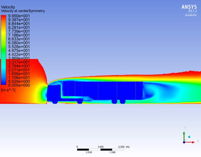
Figure 11k1: Original lorry
Figure 11k2: lorry with Deflector
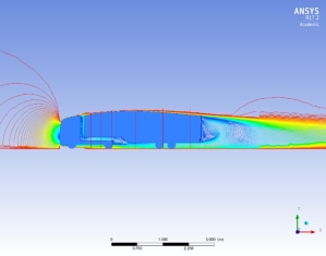
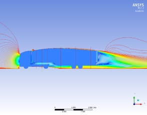
Figure 11k3: lorry with Deflector +Teardrop
Figure 11k4: lorry with All-ons
These 4 velocity contours shows different velocity distribution of different geometries.
Compared figure 11k1 and figure 11K2, it is clearly to see the flow separation above the top of front tractor of case with deflector is smaller than original case without deflector. The formation of this big eddy and huge separation will significantly increase the drag on the tractor, which will increase the fuel consumption.
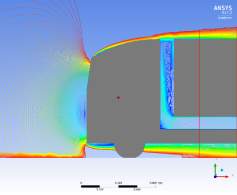
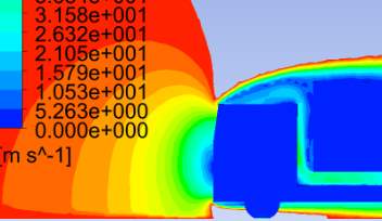
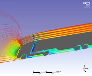
Figure 11k1a: Original lorry
Figure 11k2a: lorry with Deflector
In Figure 11k1a of original lorry and 11k2a of lorry with deflector, the flow type difference is quite clear to identify. Air flows smoothly around the tractor with no flow separations and eddy in modified lorry with deflector. However, as mentioned before, air starts to separate at tractor with huge flow separations and eddy which dramatically increase the aero drag on tractor. In the original case, the air passing through tractor surface would hit the trailer vertical surface due to the existence of height difference between tractor top and trailer top surface. This phenomenon will increase the pressure drag as well. In the lorry with deflector, the height difference is minimised so that air passes smoothly the interface between tractor and trailer, which reduces aero drag.
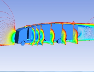
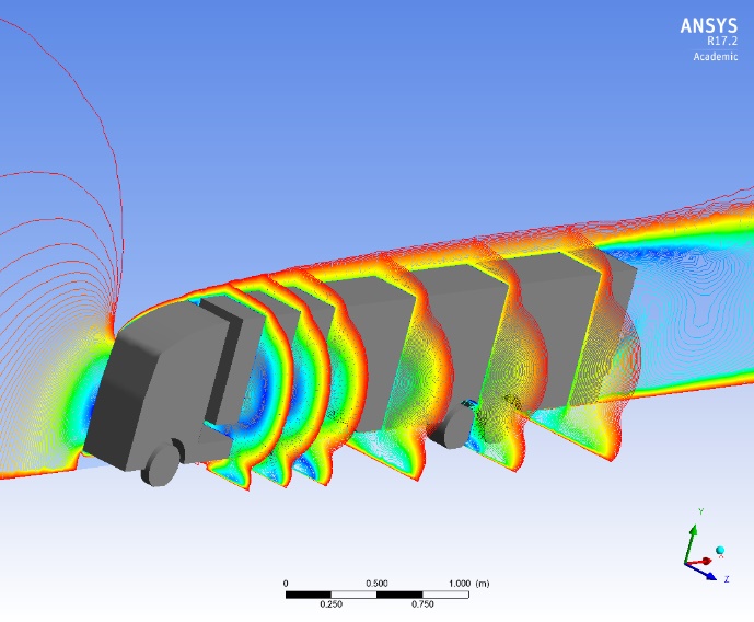
Figure11k3b: lorry with Deflector +Teardrop
Figure11k2b: lorry with Deflector
Compared with figure 11k2b and figure 11k3b, the main difference between them is if they have a streamlined surface of trailer. From these 2 velocity contours, it can be seen that air flows trailer surface with teardrop smoothly without any unnecessary turbulent flow. But in the case without Teardrop, air velocity keeps low near trailer surface region and starts to increase to until it reaches incoming flow velocity (100m/s). During this process, many turbulent flows are formed with much energy loss. As a result, lorry without teardrop will definitely waste some energy to overcome the accompanying aero drag. Thus, lorry with teardrop is considered better aerodynamic performance than lorry without it.
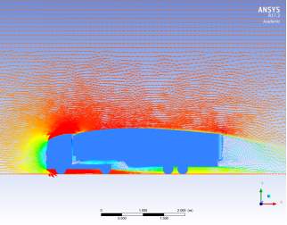


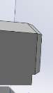

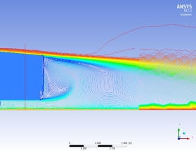
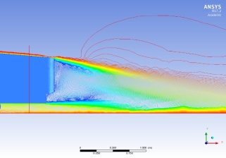
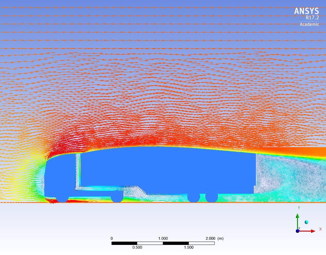
Figure 11k3c lorry with Deflector +Teardrop
Figure 11k4c lorry with All-ons
These pictures above show how does the Frame Extension influence the flow types at back region of the trailer. With a closer look at this region, it is clearly to see that the flow separation of lorry with frame extension at this region becomes smaller than lorry without this add-on. Not only air separation is decreased, but the strength of Vortex at this region is reduced as well. It needs to be mentioned that area of this region with flow circulation and vortex in the lorry with frame extension case is much smaller than case without this device.
Kinetic energy can measure strength of turbulent flow and vortices. Figure 11k3d and Figure 11k4d belowmeasure the distribution of kinetic energy of two types of lorry at different section surfaces with different distance. It is clearly to see that turbulent kinetic energy is reduced in the case of all add-on devices (Figure 11k4d), compared with case without frame extension (Figure 11k3d).
Generally speaking, this devices reduces vortex strength and formed more streamlined flow pattern at rear part of the trailer, which reduces some energy waste through reducing the formation of the vortices.
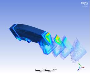
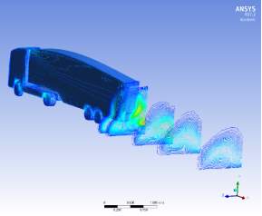
Figure 11k3d – Kinetic energy distribution lorry without Frame Extension
Figure 11k4d- Kinetic energy distribution lorry with Frame Extension
All in all, the modified lorry with all add-ons can increase aerodynamics performance in many point of views compared with original lorry without any add-ons devices.
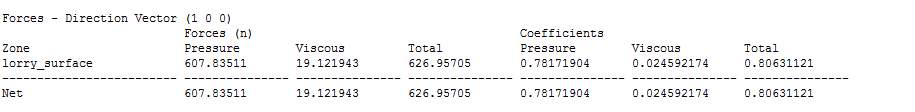
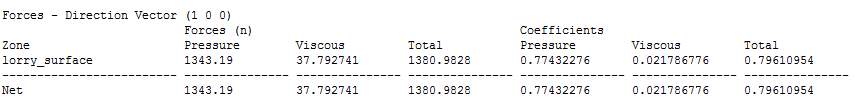
 Aerodynamics Drag (Cd) Analysis of different Lorries
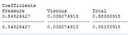
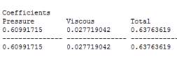
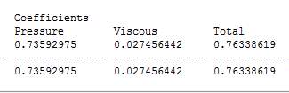
Figure 12b: Cd of Lorry (deflector)
Figure 12a: Cd of Original lorry
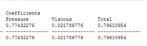
Figure 12d Cd of Lorry (deflector + Teardrop +Frame Extension)
Figure 12c: Cd of Lorry (deflector + Teardrop)
v
| Original lorry | Deflector | deflector + Teardrop | Deflector +Teardrop + Frame Extension |
| 0.796 | 0.763 | 0.638 | 0.583 |
| 0.00% | 4.15% | 19.85% | 26.76% |
Table 4: Cd of Lorries
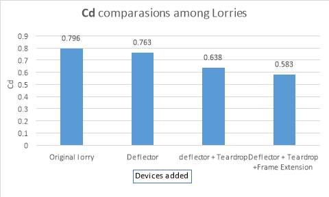
Figure 13: Cd of Different lorries
In this chart of Cd comparison, Cd of original lorry is 0.796 when travelling at speed of 90Km/h situation in the reality. Cd of lorry with deflector is 0.793 which is 4.15% smaller than original lorry, Cd of lorry with deflector and teardrop is 0.638, which is 20% less than Cd in original lorry. In terms of lorry with all add-on devices, Cd is 26.76% smaller than original lorry. Therefore, it is obvious that these devices do improve the aerodynamic performance of the Lorry and produce more streamlined flow. These lorry with add-on devices will significantly reduce aerodynamic drag.
Discussion
Through this experiment of a typical lorry using ANSYS-Fluent, the flow patterns around a typical commercial heavy is investigated and deeply understood by the author. Most flow patterns around the lorry are reasonable and practical compared with real situation in the reality. Flow types in this simulation are similar to the case of aerodynamic analysis of a lorry from the literature review study. This means the results in this simulation can be deemed as reasonable and acceptable. However, it is necessary to check the accuracy of this simulation through wind tunnel test if time and resource is enough. CFD simulation is a Black-Box which is full of unknow parameters. A correct input cannot guarantee a 100% correct output even if a perfect mesh is created. Thus, these results from CFD simulation could be considered as a reference value. More validations are still needed to be finished in other methods such as Wind tunnel test. But with the development of computer performance and relevant theory, it is possible to simulate a more accurate result in the future.
The modification of lorry geometry does increase Aerodynamic Performance of a lorry a lot. As mentioned above, the geometry with all add-on devices can reduce 26% of the aerodynamics Drag coefficient compared with conventional lorry. Credits should be given to these add-on devices due to their significant contribution to Drag reduction. However, the market considers not only technology, but it views more about cost and profits. For example, the process of assembling these add-on devices will cost both time and money, which will directly decrease the efficiency of transportation. Especially for the Aero Teardrop device, it has a curve surface on the top which is hard to install onto a conventional trailer. Similar for the frame extension devices, installing of this would take some time and human resource. All in all, there are still some factors to consider of these devices when it comes to a real market.
Reference
[1] Alam F, Chowdhury H, Moria H and Watkins S. Effects of
Vehicle Add-Ons on Aerodynamic Performance. The Proceeding of the 13th Asian Congress of Fluid Mechanics (ACFM2010), Dhaka: Bangladesh University of Engineering and Technology; 2010, p.186-189
[2] California Air Resources Board Draft California Greenhouse Gas Inventory, November 17, 2007 [cited, August 2012] http://www.arb.ca.gov/cc/inventory/inventory.htm
[3] Milne Thomson, Theoretical Aerodynamics, Dover Publications
[4] Wikipedia, (2018), “Lewis Fry Richardson”, https://en.wikipedia.org/wiki/Lewis_Fry_Richardson
[5] Jiyuan Tu, Guan-Heng Yeoh, Chaoqun Liu (2013) Computational Fluid Dynamics, Second edition. CPI group(UK) Ltd, Croydon: Butterworth-Heinemann.
[6] R.M. Wood (2004). Impact of advanced aerodynamic technology on transportation energy consumption. SAE International.
[7] Marcus Faccioni (October 14th, 2017) BIG TRUCK OF TRANSPORTATION, -, Sketched by SOLIDWORKS from GrabCAD, https://grabcad.com/library/big-truck-of-transportation-1
[8] L. Taubert, I. Wygnanski, Preliminary experiments applying active flow control
To a 1/24th scale model of a semi-trailer truck, Lecture Notes Appl. Comput.
Mech. 41 (2009) 105–113.
[9] ANSYS, Inc (November 2013) ANSYS Fluent Meshing User’s Guide, Release 15.0 edn. Southpointe November 2013 275 Technology Drive Canonsburg, PA 15317: ANSYS, Inc.
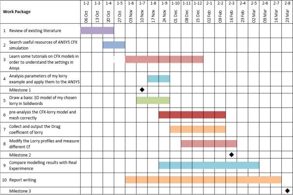
Appendix A- Schedule
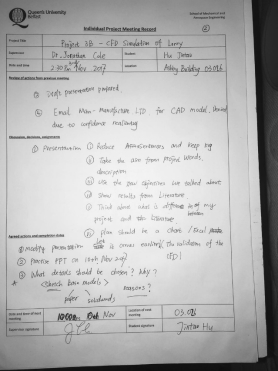
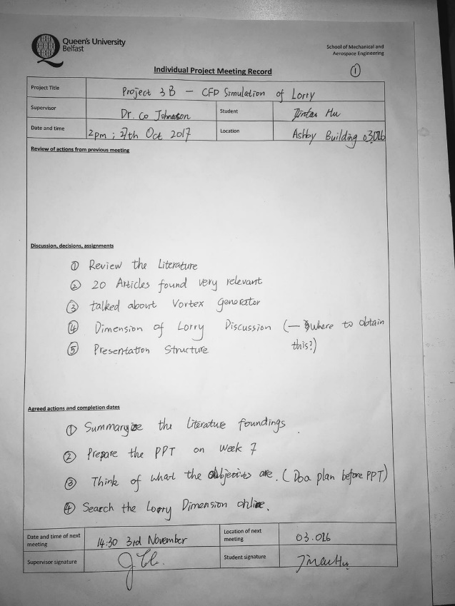
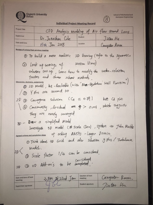
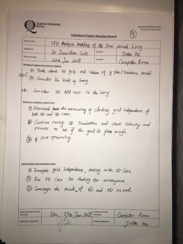
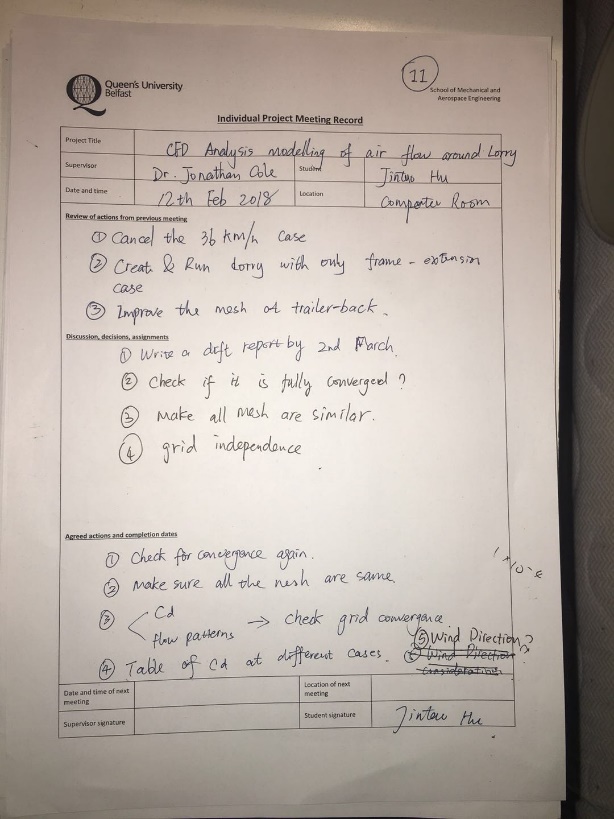
Appendix B- Meeting Record
Appendix C
Cite This Work
To export a reference to this article please select a referencing stye below:
Related Services
View all


Related Content
All TagsContent relating to: "Engineering"
Engineering is the application of scientific principles and mathematics to designing and building of structures, such as bridges or buildings, roads, machines etc. and includes a range of specialised fields.
Related Articles

DMCA / Removal Request
If you are the original writer of this dissertation and no longer wish to have your work published on the UKDiss.com website then please: