Analysis of NBA Player Performance, Popularity and Salary

ABSTRACT

National Basketball Association is a major basketball league for men in America; united of 30 teams . It is recognised by FIBA which is also known as the national governing body  for basketball in USA. NBA players are the world’s best paid athletes. NBA advance statistics are kept to estimate an individual or a team’s performance to analyse their social activities and interaction with their social network. This paper aims at finding relations to player’s salary with their performance along with their twitter follower by analysing the linear regression, PCA, SVM and Decision Tree technique.

Key Words:

Linear regression Model, PCA, SVM, Decision Tree and NBA.

Research Question

“Does engagement on social media correlate with popularity on Wikipedia?

Is follower count or social-media engagement a better predictor of popularity on Twitter?” 

Research Hypotheses

“NBA players with certain set of proficiencies/characteristics are more likely to have more twitter followers than other players”.

Introduction

Though the analyses of game-related statistics have been popular among coaches for a long time, the types of data collected and algorithm created have been constantly evolving to better serve changing analytical needs. This paper is intended to take advantage of advanced statistics, such as game played in a regular season, efficiencies against opponents, points scored, PACE, rebounds, blocks, steals, twitter followers  etc., that any team collects proprietarily in order to analyse the usefulness of these variables in characterizing and understanding the player’s contribution to their teams success.

Data Description

Gathering the NBA data represents a nontrivial software engineering problem. Knowing that the ultimate goal is to compare the social-media influence and power of NBA players, In theory, this would be an easy task, but there are a few traps to collecting NBA data. The intuitive place to start would be to go to the official web site at nba.com., that is, downloading from a web site and cleaning it up manually in  R Studio. The data set comes from a NBA advance statistics data from Kaggle

Which has 63 variables and 101 observations.

Processing the data

In order to prepare the data, data is splitting in training and testing data by using simple R code.70 percent of data was used for training and remaining data set was kept for testing the model. Finally cross validation was done to test data and check the model performance.

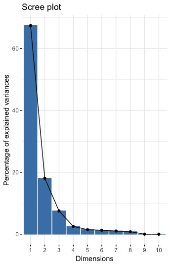
Principal Component Analysis

PCA is a dimension-reduction tool that can be used to reduce a large set of variables to a small set that still contains most of the information in the large PC1 have 67% of the variance, PC2 have 18% , PC3 have 7.5% and PC4 have 2.5% and the others are not that significant. The cumulative proportion shows that more than 97% variance is covered up to PC6.

Regression Model

Multiple linear regression , a supervised learning is used to compare the relation between the respond variables and the other dependant variables. In order to compare residuals for different observations one should take into account the fact that their variances may differ. A simple way to allow for this fact is to divide the raw residual by an estimate of its standard deviation by calculating the standardized residual.

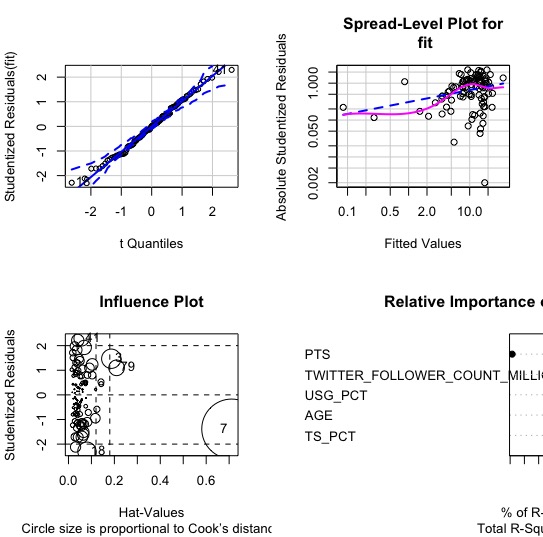
Standardized residuals are useful in detecting anomalous observations or outliers. From the above influential plot it is clear that this NBA data observation  is influential •  Size is not proportional to Cook’s distance. Its more on the right, so there is a low leverage in the model.

now build a new regression model using the ‘SALARY_MILLIONS variable and test for heteroskedasticity  by using the ‘gvlma’ package,

For Level of Significance =  0.05

Summary of the best fit:

Call:

lm(formula = SALARY_MILLIONS ~ AGE + TS_PCT + USG_PCT + PTS +

TWITTER_FOLLOWER_COUNT_MILLIONS, data = nba)

Coefficients:

(Intercept)                              AGE

4.4839                           0.5723

TS_PCT                          USG_PCT

-24.1342                         -41.3052

PTS  TWITTER_FOLLOWER_COUNT_MILLIONS

0.9497                           0.3960

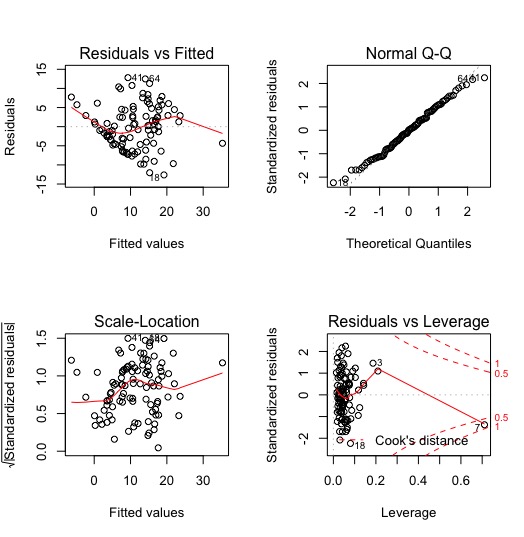
This tests for the linear model assumptions and helpfully provides information on other assumptions. In this case focus is at the heteroskedasticity decisions, which has been identified as not being satisfied. Therefore need to reject the null hypothesis and state that there is heteroskedasticity in this model at the 5% significance level.

Finally , the below table shows that the assumptions are acceptable, and therefore it clearly state that heteroskedasticity is not present in this model. Lastly, it will demonstrate that the model has corrected  graphically. As per previously, the first and third plots are the ones to look at. In the corrected plot the red lines are much more flat, and that the residuals are no longer clumped in locations. Therefore it shows  that  it has corrected heteroskedasticity in the model.

gvlma (x = fit)

	Value	p-value	Decision
Global Stat	4.8228	0.3060	Assumptions acceptable
Skewness	0.1556	0.6932	Assumptions acceptable
Kurtosis	1.3310	0.2486	Assumptions acceptable
Link Function	1.3977	0.2371	Assumptions acceptable
Heteroscedasticity	1.9384	0.1638	Assumptions acceptable

Decision and results

Call:

lm(formula = SALARY_MILLIONS ~ AGE + TS_PCT + USG_PCT + PTS +

    TWITTER_FOLLOWER_COUNT_MILLIONS, data = nba)

Residuals:

    Min      1Q  Median      3Q     Max

-12.622  -4.374   0.079   4.361  12.819

Coefficients:

                                Estimate Std. Error t value Pr(>|t|)   

(Intercept)                       4.4839    11.1064   0.404 0.687332

AGE                               0.5723     0.1590   3.600 0.000511 ***

TS_PCT                          -24.1342    13.1209  -1.839 0.069018

USG_PCT                         -41.3052    19.7657  -2.090 0.039341 *

PTS                               0.9497     0.1501   6.326 8.44e-09 ***

TWITTER_FOLLOWER_COUNT_MILLIONS   0.3960     0.1522   2.602 0.010757 *

 

Signif. codes:  0 ‘***’ 0.001 ‘**’ 0.01 ‘*’ 0.05 ‘.’ 0.1 ‘ ’ 1

Residual standard error: 5.88 on 94 degrees of freedom

Multiple R-squared: 0.5751, Adjusted R-squared: 0.5525

F-statistic: 25.44 on 5 and 94 DF, p-value: 3.815e-16

This output indicates that the fitted value is given by-

Y= 4.4839 + 0.5723X1 -24.1342X2 -41.3052X3 + 0.9497X4 + 0.3960X5

Inference in the multiple regression setting is typically performed in a number of steps. the summary statistics that the linear model yields a strong R2 result with an adjusted R2 of 0.6978

The significant F-statistics from the Wald test further confirms that the linear model decently fits the data and could potentially be used to make future forecasts .

As demonstrated in the residual vs. fitted value plot and normal Q-Q plot below, the linear model results in a very good fit except on a few data points. Data points like this will make the tail in Q-Q plot deviate from their expected position, and they should be analysed case by case. However, in general, the linear model results in a satisfactory fit from scatterplot, statistical summary and residual plots.

From the outputs of the model, there undoubtedly is a strong linear correlation between a SALARY per MILLIONS and the team PER. It makes logical sense because teams with more talented players are supposed to win proportionally more games. The relatively high R2 values and significant F-statistics confirm the goodness of fit of the model. There, however, still are some issues and complications about the model that I would like to discuss.

Welch Two Sample t-test proves that the results are statistically significant as the p-value is a lot smaller. So the alternative hypothesis is true as the difference in means is not equal to zero. In the end it shows that NBA players with certain set of proficiencies are more likely to have more twitter followers than other players.

Support Vector Machines with Radial Basis Function Kernel

76 samples

62 predictors

No pre-processing

Resampling: Cross-Validated (10 fold, repeated 3 times)

Summary of sample sizes: 68, 70, 68, 68, 68, 69, …

Resampling results across tuning parameters:

C     RMSE      Rsquared   MAE

0.25  8.258797  0.3890508  7.248933

0.50  7.939011  0.4037353  6.771456

1.00  7.447366  0.4106806  6.070366

2.00  7.228367  0.4136702  5.720482

4.00  7.110805  0.4067402  5.620212

Tuning parameter ‘sigma’ was held constant at a value of 5.150215e-07

RMSE was used to select the optimal model using the smallest value.

The final values used for the model were sigma = 5.150215e-07 and C = 4.

The SVM model gives us good results on the test data. Every player who has twitter followers is accurately assessed. According to this model, some players who do not have followers could be wrongly assessed. In relative terms, this is an acceptable misdirection consider to the nature of the problem.

The results of this model is great, it is likely that this model will  perform well. In addition, devising an efficient method of feature selection will have a great positive effect on the accuracy, specificity, and sensitivity of our model.

Players were not consistent in their game and/or not as good when they were playing on the road versus at home, or vice versa.

Teams went on long stretches of losing because of major injuries from key players, and did not bounce back quickly once those players returned to the line-up.

it is uncommon for players without high performance or maximum salary to have more followers and fans. For instance,  they have a rather effective pick-and-roll offensive system that works well for them and thus they are sitting comfortably above the linear regression line in the scatterplot.

Sometimes fan followers between two teams do not necessarily depend on the players. It is hard to factor this other factor into the model because these other factors that do not show up tangibly in players’ stats upon which our model is based.

Predictions and Analysis

After building and analysing linear models from nba data set to predict re players performance, it is clearly visible that the red and blue dots in the scatterplot represent the actual win ratios of each team at the end of  season. Yellow dots are predicted win ratios based on the model from season while the green dots are predicted win ratios based on the model from season

Since the model is in a way more biased towards players’ individual strengths, teams like the Celtics are negatively impacted and misjudged. A possible direction of further research into this topic is to find a solution to address this issue, devising a method that could capture how much better/worse players are collectively.

VALIDATION SAMPLING

The principles of data-splitting distinguish between fitting and validation samples – they are from the same data set but, at the same time, are distinct and independent from one other. Since the fitted model performs in an optimistic manner on the fitting sample, are to expect a lower performance of the model on the validation sample. The main focus is to measure the predictive performance of a model and its ability to accurately predict the outcome variable on new subjects. For the fitting sample it is interested in evaluating how well the model fits the data on which it was developed. Interest in the latter relates in particular to how much the performance ability decreases or degenerates from what was quantified in the fitting set.

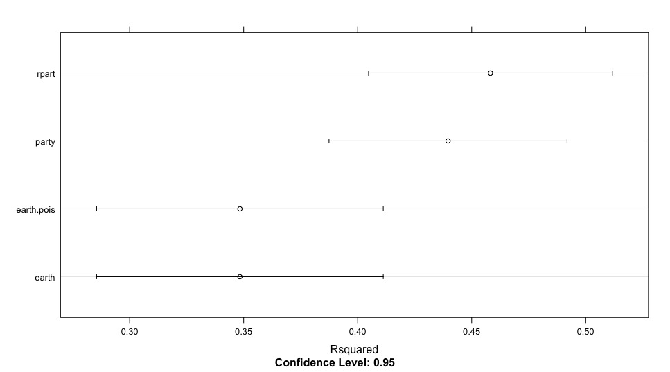
Model Performance

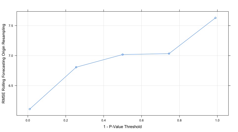
The rpart model is the winner, RMSE of the different model  from the below table and the below sensitivity plots demonstrate that the model is intuitive: Higher Salary leads to higher number of twitter follower.

The closest point of the line to the horizontal axis from the below graph represents the model with the smallest forecast errors and vice versa.

MODEL	lm.mod	earth.mod	earth.pois.mod	party.mod	rpart.mod
RMSE	44.85268	7.175672	9.99807	6.226008	6.108980

Although predicting the players contributions based on NBA advance statistics, it is impossible to get rid of the other factors involved in the game entirely. Sometimes worst player can surprisingly has more twitter followers. It is hard to analyse these factors into the model because it largely depends on the match-up and that do not show up tangibly in players’ statistics upon which our model is based. A possible mitigation is to add an additional term in the linear model to capture these factors.

Conclusion

NBA players wants to make the most money in salary should switch to teams that let them score and many NBA players do not have social Media handles and fan social engagement is a better predictor of true performance metrics than salary.

References

Gorton, B.A. Evaluation of the serve and pass in womens volleyball competition. Nfesters thesis, George Williams College, 1970.

Haberman, S.J. Analysis of scores of Ivy League football games. In S. Ladany & R. Machol (Eds.), Optimal strategies in sports. Amsterdam: New Holland, 1977.

Hildebrand, D.K., Laing, J.D. & Rosenthal, H. Prediction analysis of cross classifications. New York: John Wiley & Sons, 1977.

Hoehn, J.E. The Knox basketball test as a predictive measure of overall basketball ability in female high school basketball players. Masters thesis, Central Missouri State University, 1979.

Hopkins, D.R. Using skill tests to identify successful and unsuccessful basketball performers. Research Quarterly, 1980, 51, 381-387.

Kerlinger, F.N. & Pedhazur, E.J. Multiple regression in behavioral research. New York: Holt, Rinehart & Winston, Inc., 1973.

Kim, J.O. & Kohout, F.J. Multiple regression analysis: subprograms regression. In N.H. Nie, C.H. Hull, J.G. Jenkins, K. Steinbrenner, & D.J. Bent, (Eds.), SPSS-statistical package for the social sciences. New York: McGraw-Hill Book Co., 1975.

Lindsey, G.R. A scientific approach to strategy in baseball. In S. Ladany & R. Machol (Eds.), Optimal strategies in sports. Amsterdam: New Holland, 1977.

Miller, K. & Horky, R.J. Modern basketball for women. Columbus, Oh.: Charles E. Merrill Publishing Co., 1970.

Nie, N.H., Hull, C.H., Jenkins, J.G. Steinbrenner, K., & Bent, D.H. SPSS-statistical package for the social sciences. New York: McGraw-Hill Book Co., 1975.

Peterson, J.T. The prediction of basketball performance. California, 1980, 42, 21.

Press, S.J. & Wilson, S. Choosing between logistic regression and discriminant analysis. Journal of the American Statistical Association, 1973, 699-705.

63 Price, B. & Rao, A. A model for evaluating player performance in professional basketball. In S. Ladany & R. Machol (Eds.), Optimal strategies in sports. Amsterdam: New Holland, 1977.

Schultz, R.W. Sports and mathematics: a definition and delineation. ResearchQuarterly,1980,5J_, 37-49.

Scott, R.J. The relationship of statistical charting to team success in volleyball. listers thesis, University of California, Los Angeles, 1971.

Wilson, G.E. A study of the factors and results of effective team rebounding in high school basketball. Master’s thesis, University of Iowa, 1948.

Pragmatic AI: An Introduction to Cloud-Based Machine Learning, First Edition by Noah Gift , Published by Addison-Wesley Professional, 2018

Appendix

Variable Names

PLAYER_ID

Player unique id

PLAYER_NAME

Player’s name.

TEAM_ID

Player’s team unique id.

TEAM_ABBREVIATION

Abbreviation for the team the player is on.

AGE

Player age.

GP

Games played.

W

Games played where the team won.

L

Games played where the team lost.

W_PCT

Percentage of games played won.

MIN

Minutes played.

OFF_RATING

Player offensive rating.

DEF_RATING

Player defensive rating.

NET_RATING

Average of the offensive/defensive rating.

AST_PCT

Assist percentage.

AST_TO

Assists-to-turnovers.

AST_RATIO

Assists-to-turnovers ratio.

OREB_PCT

Offensive rebounds.

DREB_PCT

Defensive rebounds.

REB_PCT

Total rebounds.

TM_TOV_PCT

Team turnover rate.

EFG_PCT

Effective field goal percentage. This is an imputed statistic.

TS_PCT

True Shooting Percentage; an imputed measure of shooting efficiency.

USG_PCT

Usage percentage, an estimate of how often a player makes team plays.

PACE

Pace factor, an estimate of the number of possessions.

PIE

Player impact factor, a statistic roughly measuring a player’s impact on the games that they play that’s used bynba.com.

FGM

Field goals made.

FGA

Field goals attempted.

FGM_PG

Field goals made percentage.

FGA_PG

Field goals attempted percentage.

FG_PCT

Field goals total percentage.

GP_RANK

Games played, league rank.

W_RANK

Wins, league rank.

L_RANK

Losses, league rank.

W_PCT_RANK

Win percentage, league rank.

MIN_RANK

Minutes played, league rank.

OFF_RATING_RANK

Offensive rating, league rank.

DEF_RATING_RANK

Defensive rating, league rank.

NET_RATING_RANK

Net rating, league rank.

AST_PCT_RANK

Assists percentage, league rank.

AST_TO_RANK

Assists-to-turnovers, league rank.

AST_RATIO_RANK

Assist ratio, league rank.

OREB_PCT_RANK

Offensive rebounds percentage, league rank.

DREB_PCT_RANK

Defensive rebounds percentage, league rank.

REB_PCT_RANK

Rebounds percentage, league rank.

TM_TOV_PCT_RANK

Team turnover, league rank.

EFG_PCT_RANK

Effective field goal percentage, league rank.

TS_PCT_RANK

True shooting percentage, league rank.

USG_PCT_RANK

Usage percentage, league rank.

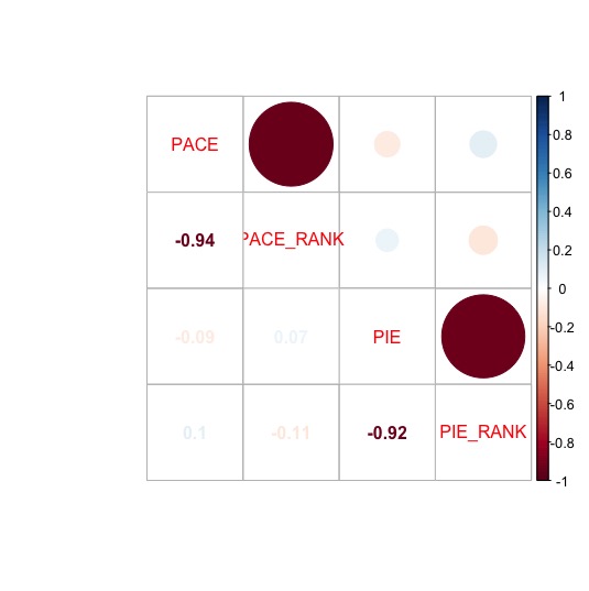
PACE_RANK

Pace score, league rank.

PIE_RANK

Player impact, league rank.

FGM_RANK

Field goals made, league rank.

FGA_RANK

Field goals attempted, league rank.

FGM_PG_RANK

Field goals made percentage, league rank.

FGA_PG_RANK

Field goal attempted percentage, league rank.

FG_PCT_RANK

Field goal percentage, league rank.

 CFID

CFPARAMS

WIKIPEDIA_HANDLE

Player’s name on Wikipedia

TWITTER_HANDLE

Twitter handle.

SALARY_MILLIONS

Salary.

PTS

Points scored.

ACTIVE_TWITTER_LAST_YEAR

Whether or not the player was active (posted) on Twitter last year.

TWITTER_FOLLOWER_COUNT_MILLIONS

Number of Twitter followers.

R CODE

nba <- read.csv(“nba1.csv”)

attach(nba)

head(nba)

summary(nba)

str(nba)

fit1 <- lm(SALARY_MILLIONS ~AGE + GP + W + L + W_PCT + NET_RATING + AST_PCT + REB_PCT + TM_TOV_PCT + TS_PCT + USG_PCT + PACE + PIE + PTS, data=nba)

fit1

library(corrplot)

cor(data.frame(GP, W, L, W_PCT))

Games <- cor(data.frame(GP, GP_RANK, W, W_RANK, L, L_RANK, W_PCT, W_PCT_RANK))

Games

corrplot.mixed(Games)

ODN <- cor(data.frame(OFF_RATING, OFF_RATING_RANK, DEF_RATING, DEF_RATING_RANK, NET_RATING, NET_RATING_RANK))

ODN

corrplot.mixed(ODN)

ASS <- cor(data.frame(AST_PCT, AST_PCT_RANK, AST_RATIO, AST_RATIO_RANK, AST_TO, AST_TO_RANK))

ASS

corrplot.mixed(ASS)

REB <- cor(data.frame(OREB_PCT, OREB_PCT_RANK, DREB_PCT, DREB_PCT_RANK, REB_PCT, REB_PCT_RANK))

REB

corrplot.mixed(REB)

a <- cor(data.frame(TM_TOV_PCT, TM_TOV_PCT_RANK, EFG_PCT, EFG_PCT_RANK, TS_PCT, TS_PCT_RANK, USG_PCT, USG_PCT_RANK))

a

corrplot.mixed(a)

b <- cor(data.frame(PACE, PACE_RANK, PIE, PIE_RANK))

b

corrplot.mixed(b)

FG <- cor(data.frame(FGM, FGM_RANK, FGA, FGA_RANK, FGM_PG, FGM_PG_RANK, FGA_PG, FGA_PG_RANK, PTS))

FG

corrplot.mixed(FG)

TWI <- cor(data.frame(ACTIVE_TWITTER_LAST_YEAR, TWITTER_FOLLOWER_COUNT_MILLIONS))

TWI

corrplot.mixed(TWI)

total <- cor(data.frame(GP, W_PCT, NET_RATING, AST_PCT, REB_PCT, TM_TOV_PCT, TS_PCT, USG_PCT, PACE, PIE, PTS, ACTIVE_TWITTER_LAST_YEAR, TWITTER_FOLLOWER_COUNT_MILLIONS))

corrplot.mixed(total)

fit2 <- lm(SALARY_MILLIONS ~ AGE + GP + W_PCT + NET_RATING + AST_PCT + REB_PCT + TM_TOV_PCT + TS_PCT + USG_PCT + PACE + PIE + PTS + ACTIVE_TWITTER_LAST_YEAR + TWITTER_FOLLOWER_COUNT_MILLIONS, data=nba)

summary(fit2)

fit3 <- lm(SALARY_MILLIONS ~ AGE + TS_PCT + USG_PCT + PTS + TWITTER_FOLLOWER_COUNT_MILLIONS,data=nba)

summary(fit3)

t.test(nba$SALARY_MILLIONS,nba$TWITTER_FOLLOWER_COUNT_MILLIONS)

#best fit model

fit <- fit3

par(mfrow=c(2,2))

plot(fit)

nba <- read.csv(“nba_2016.csv”)

set.seed(50)

sample_index <- sample(1:2, nrow(nba), replace = TRUE, prob = c(0.80, 0.20))

nba_training <- nba[sample_index == 1,]

nba_testing <- nba[sample_index == 2,]

nba_mod_r2 <- lm(SALARY_MILLIONS ~ AGE + TS_PCT + USG_PCT + PTS + TWITTER_FOLLOWER_COUNT_MILLIONS, data = nba_training)

summary(nba_mod_r2)

par(mfrow = c(1, 2))

plot(nba_mod_r2, which = c(1, 2))

predictions_adjr2 <- predict.lm(nba_mod_r2, newdata = nba_testing)

predictions_adjr2

nba_df <- data.frame(predictions = predictions_ad

jr2,

values = nba_testing$SALARY_MILLIONS)

nba_df

library(ggplot2)

ggplot(nba_df, aes(predictions, values)) +

geom_point() +

geom_smooth(method = “lm”, color = “red”) +

labs(x = “Predicted Values”, y = “Actual Values”) +

theme_minimal()

library(dplyr)

nba_df %>%

mutate(residual = predictions – values) %>%

summarize(Mean_Difference = mean(abs(residual)))

library(car)

qqPlot(fit)

durbinWatsonTest(fit)

ncvTest(fit)

spreadLevelPlot(fit)

library(gvlma)

summary(gvlma(fit))

vif(fit)

sqrt(vif(fit))>2

outlierTest(fit)

influencePlot(fit, main=”Influence Plot”,

sub=”Circle size is proportional to Cook’s distance”)

relweights <- function(fit,…){

R <- cor(fit$model)

nvar <- ncol(R)

rxx <- R[2:nvar, 2:nvar]

rxy <- R[2:nvar, 1]

svd <- eigen(rxx)

evec <- svd$vectors

ev <- svd$values

delta <- diag(sqrt(ev))

lambda <- evec %*% delta %*% t(evec)

lambdasq <- lambda ^ 2

beta <- solve(lambda) %*% rxy

rsquare <- colSums(beta ^ 2)

rawwgt <- lambdasq %*% beta ^ 2

import <- (rawwgt / rsquare) * 100

import <- as.data.frame(import)

row.names(import) <- names(fit$model[2:nvar])

names(import) <- “Weights”

import <- import[order(import),1, drop=FALSE]

dotchart(import$Weights, labels=row.names(import),

xlab=”% of R-Square”, pch=19,

main=”Relative Importance of Predictor Variables”,

sub=paste(“Total R-Square=”, round(rsquare, digits=3)),

…)

return(import)

}

relweights(fit)

nba <- subset(nba, select=c(AGE, GP, W_PCT, NET_RATING, AST_PCT, REB_PCT, TM_TOV_PCT, TS_PCT, USG_PCT, PACE, PIE, PTS, ACTIVE_TWITTER_LAST_YEAR, TWITTER_FOLLOWER_COUNT_MILLIONS))

library(leaps)

regfit.full <- regsubsets(SALARY_MILLIONS ~ ., data = nba, nvmax=14)

full.summary <- summary(regfit.full)

names(full.summary)

which.max(full.summary$rss);which.max(full.summary$adjr2);which.min(full.summary$cp);which.min(full.summary$bic)

library(ggvis)

rsq <- as.data.frame(full.summary$rsq)

names(rsq) <- “R2”

rsq %>%

ggvis(x=~ c(1:nrow(rsq)), y=~R2 ) %>%

layer_points(fill = ~ R2 ) %>%

add_axis(“y”, title = “R2”) %>%

add_axis(“x”, title = “Number of variables”)

par(mfrow=c(2,2))

plot(full.summary$rss ,xlab=”Number of Variables “,ylab=”RSS”,type=”l”)

plot(full.summary$adjr2 ,xlab=”Number of Variables “, ylab=”Adjusted RSq”,type=”l”)

# which.max(full.summary$adjr2)

points(9,full.summary$adjr2[9], col=”red”,cex=2,pch=20)

plot(full.summary$cp ,xlab=”Number of Variables “,ylab=”Cp”, type=’l’)

# which.min(full.summary$cp )

points(7,full.summary$cp[7],col=”red”,cex=2,pch=20)

plot(full.summary$bic ,xlab=”Number of Variables “,ylab=”BIC”,type=’l’)

# which.min(full.summary$bic )

points(3,full.summary$bic[3],col=”red”,cex=2,pch=20)

plot(regfit.full, scale=”adjr2″)

plot(regfit.full, scale=”Cp”)

plot(regfit.full, scale=’bic’)

library(leaps)

regfit.fwd <- regsubsets(SALARY_MILLIONS ~ ., data = nba, nvmax=14, method = ‘forward’)

fwd.summary <- summary(regfit.fwd)

names(fwd.summary)

which.max(fwd.summary$rss);which.max(fwd.summary$adjr2);which.min(fwd.summary$cp);which.min(fwd.summary$bic)

library(ggvis)

rsq <- as.data.frame(fwd.summary$rsq)

names(rsq) <- “R2”

par(mfrow=c(2,2))

plot(fwd.summary$rss ,xlab=”Number of Variables “,ylab=”RSS”,type=”l”)

plot(fwd.summary$adjr2 ,xlab=”Number of Variables “, ylab=”Adjusted RSq”,type=”l”)

# which.max(fwd.summary$adjr2)

points(8,fwd.summary$adjr2[8], col=”red”,cex=2,pch=20)

plot(fwd.summary$cp ,xlab=”Number of Variables “,ylab=”Cp”, type=’l’)

# which.min(fwd.summary$cp )

points(7,fwd.summary$cp[7],col=”red”,cex=2,pch=20)

plot(fwd.summary$bic ,xlab=”Number of Variables “,ylab=”BIC”,type=’l’)

# which.min(fwd.summary$bic )

points(3,fwd.summary$bic[3],col=”red”,cex=2,pch=20)

plot(regfit.fwd, scale=”adjr2″)

plot(regfit.fwd, scale=”Cp”)

plot(regfit.fwd, scale=’bic’)

regfit.bwd <- regsubsets(SALARY_MILLIONS ~ ., data = nba, nvmax=14, method = ‘backward’)

bwd.summary <- summary(regfit.bwd)

names(bwd.summary)

which.max(bwd.summary$rsq);which.max(bwd.summary$adjr2);which.min(bwd.summary$cp);which.min(bwd.summary$bic)

library(ggvis)

rsq <- as.data.frame(bwd.summary$rsq)

names(rsq) <- “R2”

rsq %>%

ggvis(x=~ c(1:nrow(rsq)), y=~R2 ) %>%

layer_points(fill = ~ R2 ) %>%

add_axis(“y”, title = “R2”) %>%

add_axis(“x”, title = “Number of variables”)

par(mfrow=c(2,2))

plot(bwd.summary$rss ,xlab=”Number of Variables “,ylab=”RSS”,type=”l”)

plot(bwd.summary$adjr2 ,xlab=”Number of Variables “, ylab=”Adjusted RSq”,type=”l”)

# which.max(bwd.summary$adjr2)

points(9,bwd.summary$adjr2[9], col=”red”,cex=2,pch=20)

plot(bwd.summary$cp ,xlab=”Number of Variables “,ylab=”Cp”, type=’l’)

# which.min(bwd.summary$cp )

points(7,bwd.summary$cp[7],col=”red”,cex=2,pch=20)

plot(bwd.summary$bic ,xlab=”Number of Variables “,ylab=”BIC”,type=’l’)

# which.min(reg.summary$bic )

points(3,bwd.summary$bic[3],col=”red”,cex=2,pch=20)

plot(regfit.bwd, scale=”adjr2″)

plot(regfit.bwd, scale=”Cp”)

plot(regfit.bwd, scale=’bic’)

coef(regfit.full, 7);coef(regfit.fwd, 7);coef(regfit.bwd, 7)

coef(regfit.full, 3);coef(regfit.fwd, 3);coef(regfit.bwd, 3)

###########################################################

install.packages(“factoextra”)

if(!require(devtools)) install.packages(“devtools”)

devtools::install_github(“kassambara/factoextra”)

library(factoextra)

library(“factoextra”)

data <- read.csv(“nba1.csv”)

head(data)

nba.active <- data[,c(5,6,7,8,13,24,61,62,63,60)]

##calculate the covariance matrix

cov_data <- cov(nba.active)

cov_data

eigen_data <- eigen(cov_data)

eigen_data

res.pca <- prcomp(nba.active, cor = FALSE)

res.pca

res.pca$sdev^2

summary(res.pca)

names(res.pca )

biplot (res.pca , scale =FALSE)

res.pca$rotation=-res.pca$rotation

res.pca$x=res.pca$x

biplot (res.pca , scale =FALSE)

res.pca$sdev

pr.var =res.pca$sdev^2

pr.var

pve=pr.var/sum(pr.var)

pve

screeplot(res.pca, type = “lines”)

fviz_eig(res.pca)

fviz_pca_ind(res.pca,

col.ind = “cos2”, # Color by the quality of representation

gradient.cols = c(“#00AFBB”, “#E7B800”, “#FC4E07”),

repel = TRUE     # Avoid text overlapping

)

fviz_pca_var(res.pca,

col.var = “contrib”, # Color by contributions to the PC

gradient.cols = c(“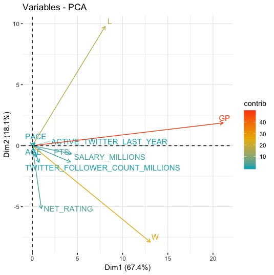#00AFBB”, “#E7B800”, “#FC4E07”),

repel = TRUE     # Avoid text overlapping

)

fviz_pca_biplot(res.pca, repel = TRUE,

col.var = “#2E9FDF”, # Variables color

col.ind = “#696969”  # Individuals color

)

library(factoextra)

#eigen value

eig.val <- get_eigenvalue(res.pca)

eig.val

# Results for Variables

res.var <- get_pca_var(res.pca)

res.var$coord          # Coordinates

res.var$contrib        # Contributions to the PCs

res.var$cos2           # Quality of representation

# Results for individuals

res.ind <- get_pca_ind(res.pca)

res.ind

res.ind$coord          # Coordinates

res.ind$contrib        # Contributions to the PCs

res.ind$cos2           # Quality of representation

# Data for the supplementary individuals

ind.sup <- nba[24:27,1:10]

ind.sup[, 1:4]

ind.sup.coord <- predict(res.pca,data =ind.sup)

ind.sup.coord[, 5:7]

# Plot of active individualsp <- fviz_pca_ind(res.pca, repel = TRUE)

p

# Add supplementary individuals

fviz_add(p, ind.sup.coord, color =”blue”)

# Centering and scaling the supplementary individuals

ind.scaled <- scale(ind.sup,

center = res.pca$center,

scale = res.pca$scale)

# Coordinates of the individividuals

coord_func <- function(ind, loadings){

r <- loadings*ind

apply(r, 2, sum)

}

pca.loadings <- res.pca$rotation

ind.sup.coord <- t(apply(ind.scaled, 1, coord_func, pca.loadings ))

ind.sup.coord[, 1:4]

groups <- as.factor(nba$GP[6:23])

fviz_pca_ind(res.pca,

col.ind = groups, # color by groups

palette = c(“#00AFBB”,  “#FC4E07”),

addEllipses = TRUE, # Concentration ellipses

ellipse.type = “confidence”,

legend.title = “Groups”,

repel = TRUE

)

l

########################################################

mydata <- read.csv(“nba1.csv”)

attach(mydata)

head(mydata)

summary(mydata)

length(mydata$SALARY_MILLIONS)

mydata_train <- mydata[1:70, ]

mydata_test <- mydata[71:100, ]

## Step 3: Training a model on the data —-

# regression tree using rpart

library(rpart)

m.rpart <- rpart(SALARY_MILLIONS ~ ., data = mydata_train)

# get basic information about the tree

m.rpart

summary(m.rpart)

fancyRpartPlot(m.rpart, main = “Players Income Level”)

# use the rpart.plot package to create a visualization

par(mfrow=c(2,1))

#install.packages(“rpart.plot”)

library(rpart.plot)

# a basic decision tree diagram

rpart.plot(m.rpart, digits = 3)

# a few adjustments to the diagram

rpart.plot(m.rpart, digits = 4, fallen.leaves = TRUE, type = 3, extra = 101)

# compare the distribution of predicted values vs. actual values

p.rpart<- predict(m.rpart, data=mydata_test)

p.rpart

mydata_test$SALARY_MILLIONS<- as.factor(mydata_test$SALARY_MILLIONS)

confusionMatrix(p.rpart, mydata_test$SALARY_MILLIONS)

summary(p.rpart)

summary(mydata_test$SALARY_MILLIONS)

# compare the correlation

cor(p.rpart, mydata_test$SALARY_MILLIONS)

# function to calculate the mean absolute error

MAE <- function(actual, predicted) {

mean(abs(actual – predicted))

}

# mean absolute error between predicted and actual values

MAE(p.rpart, mydata_test$SALARY_MILLIONS)

MAE(5.87, mydata_test$SALARY_MILLIONS)

## Step 5: Improving model performance —-

#Train the BRT Model

#install.packages(“gbm”)

library(gbm)

library(tree)

gbm.model <- gbm(formula = SALARY_MILLIONS ~ ., data = mydata_train, n.trees =1000, shrinkage = .01,bag.fraction = .9, cv.folds = 10, n.minobsinnode = 20)

gbm.model

gbmTrainPredictions = predict(object = gbm.model,

newdata = mydata_test,

n.trees = 100,

type = “response”)

#summary statistics about the predictions

summary(gbmTrainPredictions)

# compare the correlation

cor(gbmTrainPredictions, mydata_test$SALARY_MILLIONS)

#mean absolute error of predicted and true values

#(uses a custom function defined above)

MAE(mydata_test$SALARY_MILLIONS, gbmTrainPredictions)

#####################################################

nba <- read.csv(“nba1.csv”)

str(nba)

summary(nba)

library(caret)

library(e1071)

library(rpart)

library(mlbench)

da <- read.csv(“nba1.csv”)

nba<- na.omit(da)

nba

inTrain <- createDataPartition(y=SALARY_MILLIONS, p=0.75, list=FALSE)

sample_index <- sample(1:2, nrow(nba), replace = TRUE, prob = c(0.80, 0.20))

c.train <- nba[sample_index == 1,]

c.test <- nba[sample_index == 2,]

control <- trainControl(method=”repeatedcv”, number=10, repeats=3)

# train the model using support vector machines radial basis function and using the above control

model <- train(SALARY_MILLIONS ~., data=c.train, method=”svmRadial”, trControl=control, tuneLength=5)

# summarize the model

print(model)

summary(model)

#install.packages(“kernlab”)

library(kernlab)

library(caret)

length(nba$SALARY_MILLIONS)

model = ksvm(data=c.train,SALARY_MILLIONS ~.,kernel=”vanilladot”,scale=F)

model

summary(model)

pred.1 <- predict(model,c.test)

pred.1

data.frame( R2 = R2(pred.1, c.test$SALARY_MILLIONS),

RMSE = RMSE(pred.1, c.test$SALARY_MILLION),

MAE = MAE(pred.1, c.test$SALARY_MILLION))

RMSE(pred.1, c.test$SALARY_MILLION)/mean(c.test$SALARY_MILLION)

cor(pred.1, c.test$SALARY_MILLIONS)

MAE = function(actual, predicted) {

mean(abs(actual – predicted))

}

MAE(pred.1, c.test$SALARY_MILLIONS)

summary(c.test$SALARY_MILLIONS)

model.rbf = ksvm(data=c.train,SALARY_MILLIONS ~.,kernel=”rbfdot”)

pred.rbf = predict(model.rbf, c.test)

pred.rbf

cor(pred.rbf, c.test$SALARY_MILLIONS)

MAE(pred.rbf, c.test$SALARY_MILLIONS)

##########################################################################

nba <- read.csv(“nba1.csv”)

knitr::kable(head(nba))

knitr::kable(tail(nba))

library(lubridate)

nba$SALARY_MILLIONS <- as.factor(nba$SALARY_MILLIONS)

set.seed(123)

seeds <- vector(mode = “list”, length = 432)

for(i in 1:431) seeds[[i]] <- sample.int(100, 5)

library(doParallel)

library(caret)

myControl <- trainControl(method = “timeslice”,initialWindow = 36,

horizon = 12,fixedWindow = FALSE,allowParallel = TRUE,

seeds = seeds)

tuneLength.num <- 5

nba <- read.csv(“nba1.csv”)

#Leave one out cross validation – LOOCV

library(caret)

train.control <- trainControl(method = “LOOCV”)

# Train the model

lm.mod <- train(SALARY_MILLIONS ~ .,data =nba, method = “lm”,

trControl = train.control)

lm.mod

library(earth)

library(plotmo)

library(plotrix)

library(TeachingDemos)

earth.mod <- train(SALARY_MILLIONS ~ .,data =nba,method = “earth”,trControl = myControl,tuneLength=tuneLength.num)

earth.mod

earth.pois.mod <- train(SALARY_MILLIONS ~ .,

data = nba,

method = “earth”,

glm=list(family=poisson),

trControl = myControl,

tuneLength=tuneLength.num)

earth.pois.mod

library(rpart)

rpart.mod <- train(SALARY_MILLIONS ~ .,data = nba,method = “rpart”,trControl = myControl,tuneLength=tuneLength.num)

rpart.mod

library(party)

library(grid)

library(mvtnorm)

library(modeltools)

library(stats4)

library(strucchange)

library(zoo)

party.mod <- train(SALARY_MILLIONS ~ .,data = nba, method = “ctree”,trControl = myControl,tuneLength=tuneLength.num)

party.mod

resamps <- resamples(list(earth=earth.mod,earth.pois=earth.pois.mod,rpart=rpart.mod,party=party.mod))

resamps

ss <- summary(resamps)

ss

knitr::kable(ss[[3]]$Rsquared)

resamps$metrics

library(lattice)

trellis.par.set(caretTheme())

dotplot(resamps, metric = “Rsquared”)

library(party)

library(grid)

library(mvtnorm)

library(modeltools)

library(stats4)

library(strucchange)

library(zoo)

party.mod$finalModel

#party.mod

plot(party.mod)