Effect of Depth on Benthic Community Composition

The Effect of Depth in the abundance and biomass of the benthonic community in the Red Wharf Bay

1. INTRODUCTION

In marine ecosystems fishing represents the biggest anthropogenic impact, bottom fishing have a strong impact on the seafloor, altering physical habitat characteristics, sedimentation and nutrient cycling (Frid, C. L. J., et al., 2000; Macer,C.T., 1967)

Benthic communities, animals dwelling within the sediment, are related to some sediment parameters such as substrate type, grain size and organic content (Galanidi, M., et al., n.d; Warwick & Uncles., 1980). The disturbance of sediment by biological organisms, bioturbation, also has an important effect on the composition of the benthic community (Warwick & Uncles., 1980) who is as well, an important indicator of anthropogenic and environmental impacts (Callaway, 2002).

There is an important paper of the environmental factors in the community composition. The tidal currents in some regions of the Irish Sea create a transport of sand from the open sea to estuaries or embayment (Mackie, A.S.Y., 1990) and with the input of sediment from rivers, form an alteration of the sediment that can influence in the composition of the benthic community. Other factors related with depth such as sunlight radiation to the bottom, wave action and wind waves, had an important roll over the community composition (Kershaw et al., 2014). More environmental factors such as temperature or plankton blooms can also affect the community composition (Mackie, A.S.Y., 1990).

Red Wharf Bay on the coast of Anglesey in North Wales has a lot of diversity throughout the food chain (Macer,C.T., 1967). Different benthic communities can be identified according with the type of sediment. The Venus community associated with fine sand and coarser sand, the Abra community associated with mud, smooth muddy san and mixed of gravel and sand and the Modiolus community founded on the rock floors and in areas with strong currents (A.S.Y.,Mackie., 1990; Warwick & Uncles, 1980)

The object of the present study was to determine the effect of depth in the community composition and in the biomass of the Phylum Mollusca. Experiments were conducted In Red Wharf Bay to test the community composition at different depths and as a consequence, at different temperatures and type of sediment.

2. METHODS

The study area (Fig. 1) was located in the Red Wharf Bay in the Isle of Anglesey in North West Wales.  The bay is sheltered from the prevailing wind (south-west) and the main presence of benthic community is in muddy habitats (Macer,C.T., 1967). The structure of benthic communities is linked with the sedimentary environment, such as grain size and organic content ((M. Galanidi, et al., n.d). In the case of the Red Wharf Bay, the tides and wind-waves are important environmental factors to consider as an influence of the type of sediment in the area (Warwick & Uncles, 1980).

Survey design

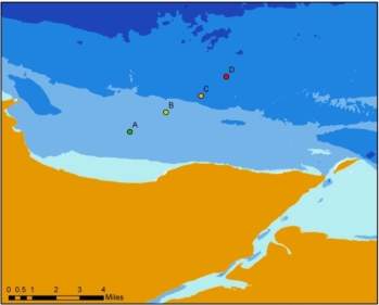
Figure 1. Map of the Red Wharf Bay where 32 samples of sediment were collected in the different sites A, B, C, D. The 10^th October, 16 samples were taken in the site D and C, 8 of the samples were collected at the site D (53˚22’19”N, 04˚05’55”W), at an average depth of 25.3 meters. The other 8 samples collected that day, were taken at site C (53˚21’37” N, 04˚06’51”W) and at an average depth of 21,5 meters. The 11^th October 8 samples were collected at site A (53˚20´18″ N, 04˚09´27″W) with an average depth of 10.1 meters. Finally, the last 8 samples collected were in an average depth of 16.1 meters at site B (53˚21’01”N, 04˚08’08”W).

Statistical analysis

The data of the community composition of the 32 samples collected were treated for further analysis using PRIMER v.5 software package.

A data matrix to analyze similarity between points was obtained from the square root transform (sqrt), of the original community data and with the use of a Resemblance analysis (Hinz et al., 2011). Differences between sites were tested by ANOSIM analysis through individual contrast and between sites, where a positive number of R (-1, 1) suggest a higher similarity (Clarke & Warwick, 2001). Cluster analysis was performed using the Bray-Curtis index of similarity to find the similar samples within the same or different group (Kaiser et al., 2006). A graphic of the samples was created by a Multidimensional scaling (MDS) analysis to show the representation of the similarities between the samples. The most abundant species in the different sites was analyzed through a Simper analysis of the data matrix obtained by Resemblance analysis; the most abundant species in a comparison between sites was also obtained. Finally, from the original data of the community composition, we obtained a dominance curve from the sum of the species in each site (Clarke & Warwick, 2001).

SPSS predictive analysis software was also used with the data of the community composition obtained through Diverse analysis with PRIMER v.5 to reduce the multivariate data into a single index, which can be statistically analyze with univariate analysis. The single data obtained from the original community composition data is the number of species (S), total individuals (N), species richness (d), pielou’s evenness (J´), Shannon index (H´) and Simpson index (D) (Kaiser et al., 2004) An analysis of variance (One-way ANOVA), a parametric test of univariate data, was tested with a previous Levene’s test (Homogeneity of Variance) to determine the assumption of homogeneity (Dytham, 2015).

If p-value obtained in the Homogeneity of Variance test was less than 0.05 a transform of the data (sqrt) was needed before ran the test again. If the p-value was still less than 0.05, a non-parametric test (Kruskall-Wallis) equivalent to one-way ANOVA was tested. Also, to indicate the sites sampled with a significant difference, a Post-hoc test (Mann-Whitney U-Test) were tested in which the sites 1-4 (A-D) were needed to be defined and compared. This test provided an output value (U) and a p-value that establish the similarity between the samples (Dytham, 2015). If p-value in the Levene’s test was more than 0.05 the Analysis of variance (One-way ANOVA) was tested to obtain the statistical significance of the results obtained in the community composition in the different sites.

An Analysis of variance (One-way ANOVA) of the 5 most abundant species in the community was tested to obtain the significance of the sites.

The Biomass data of the samples collected, Mollusca, Crustacea, Polychaeta and Echinodermata were analyzed with the statistical PRIMER v.5 and SPSS software.

A data matrix to analyze similarity between the sites, with ANOSIM analysis, was obtained from the transform (sqrt) of the original biomass data through Resemblance analysis (Spencer, Kaiser, & Edwards, 1998). A graphic of the phylum Mollusca was created by a Multidimensional scaling (MDS) analysis to test the similarities between the samples in the different sites (Clarke & Gorley, 2006; Clarke & Warwick, 2001).

A Levene’s test (Homogeneity of Variance) was also tested with SPSS software, with the original data of the phylum Mollusca; to determine the assumption of homogeneity between the sites, as the p-value obtained was 0.000 > 0.05 the analysis of variance (One-way ANOVA) was also tested to determine the significance of the Mollusca biomass at the different sites (Dytham, 2015).

Finally, the environmental data were analyzed with the statistical PRIMER v.5. A pretreatment (Normalise) of the data was needed, as the original data was in different units. Like with the abundance and biomass analysis, a data matrix of the environmental data was created with the Resemblance analysis and an ANOSIM analysis was run to analyze the similarity between the sites (Clarke & Warwick, 2001).

A Relate test, a non-parametric is used to test the relation between the environmental data and the biological data. To do the relation, it compares the Bray-Curtis resemblance matrix for the biological data with the Euclidean matrix for the environmental data. The obtained rank correlation (Rho), showed a not correlation between the environmental data and the biological data if the value is close to zero (Clarke & Gorley, 2006). Finally, a Best test was also tested to compare the environmental and the biological data comparing all the variables, depth, temperature and types of sediment were compared for that study. The results obtained for that study showed the more related variable with the biological data (Clarke & Gorley, 2006; Clarke & Warwick, 2001).

3. RESULTS

3.1 Abundance

ANOSIM and Pairwise test (Table 1) showed the difference between the sites where the samples were collected. With an R= 0.383 and a p-value= 0.001 of the ANOSIM test, revealed a significant (p-value < 0.05) difference between the community in the sites. The Pairwise test (Table1) showed a significant difference between the sites except in the comparison of the sites 2, 4 where R= 0.127 (R ≈ 0) and p-value= 0.079 (p-value > 0.05) and 3,4 where R= -0.012 (R<0) and the p-value= 0.533 (p-value > 0.05) where the results obtained revealed that the community composition between the sites 2, 4 and 3, 4 were not significantly different.

Table 1: Results obtained from the Pairwise test (p-value = 0.05) in the different sites. Where the depth range of the sites is: site 1, 9-10 meters, site 2, 15-17 meters, site 3, 21-22 meters and site 4, 24-27 meters.

Sites	R	p-value
1, 2	0.439	0.003
1, 3	0.925	0.001
1, 4	0.576	0.001
2, 3	0.145	0.046
2, 4	0.127	0.079
3, 4	-0.012	0.533

Cluster analysis (Fig. 2) from the Bray-Curtis data matrix revealed a global high difference between the community compositions in the different sites. An elevated percentage of similarity (45%) is also shown between 7 of the samples in the site 1 it also happened between two samples collected in site 3. Where site 1 corresponds to the depth range of 9-10 meters, site 2 depth range 15-17 meters, site 3, 21-22 meters and site 4 corresponds to the depth range of 24-27 meters.

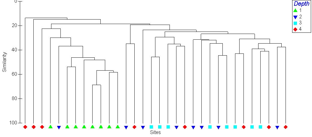
Figure 2: Cluster dendrogram from the similarities of the community composition in the 4 different sites sampled in Red Wharf Bay based on the percentage of similarity of Bray-Curtis.

The confidence interval (±95%) of the results obtained in the Diverse test (Table 2) showed the significant difference between the abundance of the benthic community in the different sites sampled. The data were analyzed with one-way analysis of variance after tested out the Levene’s test, obtaining a p-value > 0.05 in all the variables. A higher presence of individuals is shown in the depth range of 21-22 meters. Also, a result of a significant difference (p-value< 0.05) of the total individuals among the different depths is shown in the results of the test ANOVA with an F(3)= 4.251, p-value= 0.014. A higher presence of total species was also shown in the depth range of 21-22 meters; the results of the test ANOVA, F (3) = 3.986, p-value = 0.018, tested a significant difference between the total species present in the different depth range.  The results obtained from the diversity indices were significant differences between the different depth range as all the result from the ANOVA test (df= 3) are < 0.05.  After the ANOVA test, a Post hoc testing was run, HSD Tukey test to identify the groups that are significantly different. For the total individuals, with a standard error= 7.472, the samples from site 3 are significant different with samples from site 4 (mean difference (m.d) = 25.625) For the total species, with a standard error = 2.346, the samples from the site 1 are significantly different with the samples from site 2 (m.d= -7.125; p-value= 0.025) and site 3 (m.d= -6.500; p-value= 0.046). For the Pielou’s Evenness (Std. Error= 0.565) the samples from the site 1 are significantly different with the samples from site 2 (m.d= 2.073; p-value= 0.005). For the variable of the species richness (Std. Error= 0.4326) the site 1 is significantly different from site 4 (m.d= 1.288; p-value= 0.029).  The Shannon-Wiener Index a significant difference is showed with a Std. Error= 0.195 between the site 1 and the site 2 (m.d=0.720; p-value= 0.05) and between the site 1 and 3 (m.d= 0.622; p-value= 0.018).

Table 2: Table of the mean abundances and diversity indices (± 95% confidence interval) of the benthic community composition sampled at the different sites, depth range. Also results of the one-way analysis of variance (ANOVA)

Depth range	9 – 10 meters	15 – 17 meters	21 – 22 meters	24-27 meters	F	P
n	8	8	8	8
Total individuals	45.99±26.01	40.86±28.14	64.14±34.86	36.12±18.88	4.251	0.014
Total species	11.87±7.13	20.51±12.49	21.28±14.72	17.64±11.36	3.986	0.018
Diversity indices
Pielou’s Evenness	0.85±0.74	0.94±0.83	0.98±0.83	0.95±0.85	3.427	0.031
Species Richness	2,86±1.91	5.36±3.50	5.18±3.47	4.59±3.01	4.806	0.008
Shannon-Wiener	1.84±1.58	2.74±2.08	2.68±2.11	2.61±2.01	5.372	0.05
Simpson’s	0.83±0.74	0.96±0.84	0.96±0.83	0.95±0.85	4.816	0.08

The five species of the benthic community with the highest % of Contribution obtained in the Simper analysis (Table 3) were chosen for further analysis with SPSS. One-way analysis variance (ANOVA) was tested with Nephtys spp. obtaining an F(3)= 1.893 and a p-value= 0.154 showing a non-significant difference between the abundance of that species in the different sites sampled.  Test ANOVA was also tested for the specie Ophiura ophiura (F(3)= 4.697; p-value= 0.009) showing a significant difference between the sites 1 and 3 with a Std. error= 0.586 (m.d=1.750 ; p-value= 0.028) and between the sites 1 and 4 (m.d=2; p-value= 0.010). The species Nucula spp. was tested with an ANOVA test after transforming (sqrt) the data when the p-value of Levene test < 0.05. The result of the one- way ANOVA (F(3)= 27.017; p-value= 0.000) showed a high significant difference of the abundance of that specie between all the different sites (Std. Error= 0.432; m.d (1,2)= 3.06, m.d(1,3)= 2.83, m.d(1,4)= 3.49; p-value= 0.000).

Non-parametric procedures (Kruskal-Wallis test) were tested with the specie Abra alba (H(3)= 12.817, p-value= 0.005) showing a significant difference between the abundance of the specie in the different sites sampled. The results obtained from the specie Lagis Koreni (H(3)= 8.528, p-value= 0.036) also showed a significant difference between the sites sampled. To determine the sites that are significantly different, a Mann-Whitney test was run for those species. The results obtained in Abra alba showed a significant difference between all the different sites; p-value < 0.05.(Site 1-2: U=8.500, p-value (2-tailed)= 0.011, p-value [2*(1-tailed)]= 0.010.; site 1-3: U=5.000, p-value (2-tailed)= 0.002, p-value [2*(1-tailed)]= 0.003.; site 1-4: U= 11.500, p-value (2-tailed)= 0.026, p-value [2*(1-tailed)]= 0.028). The results obtained in Lagis koreni showed a significant difference (p-value< 0.05) between the samples collected in the site 2 and 4; (U= 13.500, p-value (2-tailed)= 0.026, p-value [2*(1-tailed)]= 0.05).

Table 3: Table of the results obtained from the analysis using one-way analysis variance (ANOVA) or a Kruskal-Wallis test. ¹ root transformed (sqrt) data. ^a,b,c,d Means are equally based on HSD Tukey test. Highlighted data were analyzed using non-parametric procedures.

Specie	F/H	p-value
Nepthys spp.	1.893	0.154
Ophiura ophiura	4.697	0.009a,c,d
Nucula spp. 1	27.017	0.000a,b,c,d
Abra alba	12.817	0.005
Lagis koreni	8.528	0.036

A cumulative dominance plot (Fig.3) was tested from the sum of the abundance of the samples from the original community composition data in the different sites. The benthic community obtained in the site 2 is the richness of species as shown in the dominance plot, with a value of 90 in the species rank. The diversity of species obtained in the sites 3 and 4 are close to the same value of 60 in the species rank. The diversity in the site 1 even though the cumulative % of dominance is higher, the species rank showed the less diversity between the 4 sites with a value of 40.

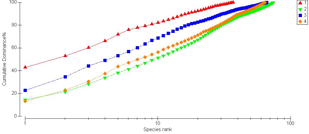
Figure 3: Cumulative Dominance (%) plot of the benthic community composition from the samples collected in different sites and in different depths.

3.2. Biomass

The results of biomass of the phylum Mollusc showed an average of 10.411 grams in the samples collected in the site 1, 1.009 grams in site 2, 2.183 grams in site 3 and 0.210 grams in the samples of Mollusca collected in site 4 (Figure 4).  The error bars in figure 4 represent the 95% confidence interval (CI) and because the error bars represented don’t overlap, a significant difference between the sites sampled is expected (p < 0.005).

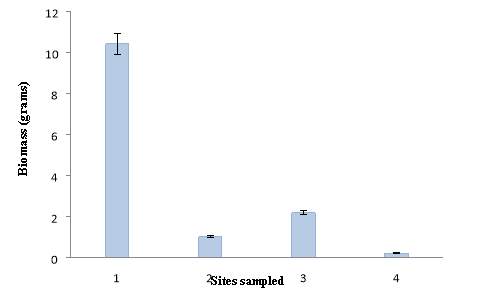
Figure 4: Bar chart of the biomass (grams) of the phylum Mollusc collected from the samples at the different range of depth.

A significant overall difference is observed (figure 5) between the different sites (a,b,c,d in the graph) where the samples were collected. The samples collected in the site 1; in particular, the samples a1, a4 and a7 have the higher biomass in contrast with the other samples. Also, the samples c5 and c6 from site 3 also have a high biomass in comparison with other collected in site 2 and 4.

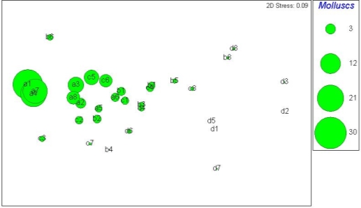
Figure 5: Multidimensional scaling (MDS) analysis to show the representation of the similarities between the Mollusc biomass in the samples collected in the different sites. The green circle with bigger diameter showed the higher biomass collected.

ANOSIM and Pairwise test were tested with the biomass data to determine the difference between the sites where the samples were collected. The ANOSIM test showed a significant difference between the biomass in the different sites (R= 0.267, p-value= 0.001).

The results obtained from the Pairwise test (Table 4) showed a significant difference between the sites except for the comparison between the sites 1,3 where R= 0.133 (R ≈ 0) and p-value= 0.091 (>0.05) and 2,3 where R= -0.037 (R<0) and p-value= 0.624 (>0.05). These results showed that there is not a significant difference of the biomass between the sites 1, 3 and 2, 3.

Table 4: Results obtained from the Pairwise test (p-value = 0.05) in the different sites.

Sites	R	p-value
1,2	0.33	0.011
1,3	0.133	0.091
1,4	0.763	0.001
2,3	-0.037	0.624
2,4	0.171	0.048
3,4	0.347	0.003

Non-parametric procedures (Kruskal-Wallis test) were tested with the Mollusc biomass (H(3)= 19.859, p-value= 0.000) showing a significant difference between the biomass of the phylum Mollusca in the different sites sampled. To determine the sites that are significantly different, a Mann-Whitney test was run for the Mollusc biomass; the results showed a significant difference between all the sites sampled; Between the site 1,2 ( U= 3, p-value (2-tailed)= 0.002, p-value [2*(1-tailed)]= 0.001); site 1,3 (U=10, p-value (2-tailed)= 0.021, p-value [2*(1-tailed)]= 0.021); site 1,4 (U=0, p-value (2-tailed)= 0.001, p-value [2*(1-tailed)]= 0.000); site 2,4 (U=9, p-value(2-tailed)= 0.016, p-value [2*(1-tailed)]= 0.015), where the p-value < 0.05 in all the different sites showed a significant difference of the biomass in the phylum Mollusca.

3.3 Environmental data

The Relate test results of the comparison between the abundance and the environmental data showed that the value from the rank correlation (Rho) 0.371, close to 0, described a low relation between the data, even though, with a p-value= 0.001, a significant relation (p-value < 0.05)  between the environmental data and the abundance was showed.

A Best test was tested to determine the variables of the environmental data more related with the abundance in the different sites sampled. A higher relation was observed with the variables depth and coarse sediment. With a correlation= 0.419 for variable depth and 0.401 for coarse sediment and depth. The lowest correlation is observed with the variable Temperature with a value of correlation = 0.377.

The Relate test results of the comparison between the biomass and the environmental data showed a non-significant relation between the data. With Rho= 0.122, close to 0, and a p-value= 0.052 (p-value > 0.05).  Therefore, a Best test was not needed to determine the variable from environmental data with a higher relation with the biomass obtained in the different sites.

5. DISCUSSION

The purpose of the experiment has been to determine the relationship between the environmental factors and the community composition, 32 samples in 4 different sites at different depths were taken in Red Wharf Bay to achieve this aims. The epifaunal survey has a particular value for the community classification (H.L., Rees et al., 1999)

Non-parametric analysis of the abundance of the benthic community showed that there was not similarity between the samples collected at different depths (sites). The highest number of individuals of the benthic community was found in the depth range of 21-22 meters followed by the depth range of 9-10 meters. These results are similar to those noted by Kaiser et al., 2006 in their study of distribution and behavior of Common Scoter where they defined their feeding are depths less than 20 meters.

The results of the non-parametric test of the relation between the environmental data and the abundance showed a significant relation between the data, being the variables depth and type of sediment the ones that present the highest level of significance. Community composition is physically controlled by environmental factors (Warwick & Uncles., 1980) The importance of the type of sediment to determine the benthic community composition has been found in different studies like Warwick and uncles 1980 where the analyzed areas where determined depended on the type of sediment and diversity of species. Other studies like Robinson et al., 2012 or Seiderer and Newell., 1999 where they analysed the evidence of the correspondence between the sediment composition and the distribution of the benthic community.

The results from the cumulative dominance plot showed that from the samples collected at different depths, the richness of species from the benthic community was showed at site 2, range depth of 15-17 meters matching again with the distribution of feeding area of the Common scoter (Kaiser et al., 2006)

Five species with the highest % of Contribution where chosen for further analysis; Nepthys spp., Ophiura ophiura, Nucula spp., Abra alba and Lagis Koreni. In other studies like; Capasso. E., 2010, Hinz et al., 2011 and Rees, H L., 1999, those species were also found in a high % of Conttribution. In the different studies, those species were found at different depths for e.g.; Nephtys sp.. was found at depths of 34, 30 and 57 meters, Ophiura ophiura was found at the depth of 20 meters, as Lagis Koreni that was also found at the depth of 20 meters, Nucula spp. was found at the depth of 20 and 33 meters and finally Abra alba was found at the depths of 69, 33 and 57 meters. Despite the results showed in the studies showed a representation of those 5 species in a wide range of depth, in the results obtained after the experiment in Red Wharf Bay, a significance difference between the abundance of 4 of the 5species studied was showed between the different sites samples, between the different depths. For Nepthys spp. A non-significance difference of abundance was observed between the sites. For Ophiura ophiura, a significance difference was observed between the sites 1 and 3 and between sites 1 and 4, so between the range depth of 9-10 meters, 21-22 meters and 24-27 meters. For Lagis koreni a sifnificance difference was observed for range depth of 15.17 meters and 24-27 meters. For Nucula spp. and Abra alba a high significance difference was observed between all the depths sampled; 9-10, 15-17, 21-22 and 24-27 meters.

Non-parametric analyses were also tested with the biomass obtained from the Phylum Mollusc at the different sites sampled. From the different biomass obtained, Mollusc, Crustaceans, Polychaeta and Echinodermanta. The Phyllum Mollusc was chosen because of their importance as in for every study the percentatge value for the occurrence of mollusc exceeded 90% and 88% for bivalvas(Capasso, E., et al.,  2009; Kaiser et al., 2006). In the study done in Red Wharf Bay, a significant overall difference between the biomass in the different sites was found, being the site 1, depth 9-10 meters, with the highest average of grams.

The results of the non-parametric test of the relation between the environmental data and the biomass showed a non-significant relation between the data.  These results are not the one expected in comparison with other studies like Davis, T.R., 2017 where explained the influence of the physical gradients in the Phylum Mollusc and in particular the importance of depth.

References 

A.S.Y., M. (1990). Offshore benthic communities of the Irish Sea, 80(1), 169.218.

Callaway, R. (2002). Diversity and community structure of epibenthic invertebrates and fish in the North Sea. ICES Journal of Marine Science, 59(6), 1199–1214. https://doi.org/10.1006/jmsc.2002.1288

Capasso, E., Jenkins, S. R. R., Frost, M., & Hinz, H. (2009). Investigation of benthic community change over a century-wide scale in the western English Channel. Journal of the Marine Biological Association of the United Kingdom, 90(6), 1161–1172. https://doi.org/10.1017/S0025315409991020

Clarke, K. R., & Gorley, R. N. (2006). PRIMER v6: User Manual/Tutorial. PRIMER-E, Plymouth UK, 192 p. https://doi.org/10.1111/j.1442-9993.1993.tb00438.x

Clarke, K. R., & Warwick, R. M. (2001). Change in marine communities: an approach to statistical analysis and interpretation, 2nd edition. PRIMER-E, Plymouth UK. https://doi.org/1

Dytham, C. (2015). Choosing and Using Statistics – A Biologist’s Guide. Journal of Ecology (Vol. 1). https://doi.org/10.1017/CBO9781107415324.004

Frid. C. L. J. , . Harwood. K. Hall. G, S. J, A., & A., H. J. (2000). Long-term changes in the benthic communities on North Sea fishing grounds. ICES Journal of Marine Science, 57(5), 1303–1309. https://doi.org/10.1006/jmsc.2000.0900

Kaiser, M. J., Bergmann, M., Hinz, H., Galanidi, M., Shucksmith, R., Rees, E. I. S., … Ramsay, K. (2004). Demersal fish and epifauna associated with sandbank habitats. Estuarine, Coastal and Shelf Science, 60(3), 445–456. https://doi.org/10.1016/j.ecss.2004.02.005

Kaiser, M. J., Galanidi, M., Showler, D. A., Elliott, A. J., Caldow, R. W. G., Rees, E. I. S., … Sutherland, W. J. (2006). Distribution and behaviour of Common Scoter (Melanitta nigra) relative to prey resources and environmental parameters. Ibis, 148(s1), 110–128. https://doi.org/10.1111/j.1474-919X.2006.00517.x

Kershaw, S., Griffiths, J., Polisi, T., Walker, D., Parks, R., Vogt, F., … Cook, A. (2014). CLASSIFICATION OF BIVALVE MOLLUSC PRODUCTION AREAS IN ENGLAND AND WALES. Retrieved from http://www.cefas.defra.gov.uk/our-science/animal-health-and-food-safety/food-safety/sanitary-surveys/england-and-wales.aspx

M. Galanidi, M. J. Kaiser, S. Neill, A.J. Elliott, R. W. G. C. & W. J. S. (n.d.). Wave erosion as a key predictor of benthic prey resources for coastal diving seabirds.

Macer, C. T. (1967). The food web in Red Wharf Bay (North Wales) with particular reference to young plaice (Pleuronectes platessa). Helgolander Wissenschaftliche Meeresuntersuchungen, 15(1–4), 560–573. https://doi.org/10.1007/BF01618651

Rees, H. L., Pendle, M. a, Waldock, R., Limpenny, D. S., & Boyd, S. E. (1999). A comparison of benthic biodiversity in the North Sea, English Channel, and Celtic Seas. ICES Journal of Marine Science, 56(2), 228–246. https://doi.org/10.1006/jmsc.1998.0438

Spencer, B. E., Kaiser, M. J., & Edwards, D. B. (1998). Intertidal clam harvesting: Benthic community change and recovery. Aquaculture Research, 29(6), 429–437. https://doi.org/10.1046/j.1365-2109.1998.00221.x

Warwick, R., & Uncles, R. (1980). Distribution of Benthic Macrofauna Associations in the Bristol Channel in Relation to Tidal Stress . Marine Ecology Progress Series, 3, 97–103. https://doi.org/10.3354/meps003097