Dissertation on Evaluating Habitat Quality for Fish Conservation
Info: 22575 words (90 pages) Dissertation
Published: 23rd Nov 2021
Tagged: Environmental StudiesEcology
The Performance of a bioenergetics model in a system with an abundant population of salmonids: A case study of cutthroat trout in the Logan River, Utah
ABSTRACT
Widespread habitat degradation and fragmentation has significantly altered the distribution and abundance of salmonids across the Western United States. To effectively recover and manage these fish populations, managers need tools that evaluate habitat quality in physically diverse streams and watersheds. For salmonids, drift-foraging, bioenergetics models are increasingly being used to evaluate habitat quality and quantity, as well as carrying capacity of sites. However, many of these bioenergetics models have been developed and applied for salmonids at sites whose populations are well below carrying capacity. It is essential to test the predictions of these models on populations of salmonids that are abundant. In this case study, I tested a bioenergetics model that has recently been applied to inform habitat management in the Western US on cutthroat trout. I surveyed the spatial location of Bonneville cutthroat trout (BCT; Oncorhynchus clarkiiutah) in the Logan River, Utah, a system where one of the most abundant populations of BCT reside, to determine if the fish were using locations with a high energetic value, predicted by a Net Rate of Energy Intake (NREI) modeling framework. I conducted snorkel surveys in both summer and fall to assess whether the modeled predictions were robust to changes in drift, temperature, or discharge. I also tested whether sampling estimates of BCT abundance were related to the NREI model predicted carrying capacity, or the proportion of suitable habitat (i.e. NREI > 0.0 J·s-1). Last of all, I tested whether the observed biomass of BCT was related to the mean NREI at each study site. I found that the majority of observed fish occupied focal positions that (i) had positive NREI and (ii) had NREI values that were significantly greater than the site mean. I also found that the simulated carrying capacity predicted for each site was significantly, positively related with the maximum BCT densities observed between 2001 and 2015 (R2=0.93, P=0.009). However, observed BCT densities and biomass were uncorrelated with the proportion of suitable habitat and the mean NREI at sites, respectively. I concluded that drift foraging bioenergetics models are a useful tool for pin-pointing bioenergetically favorable locations within sites and discriminating capacity between sites for BCT and other similar trout species.
PUBLIC ABSTRACT
Widespread habitat degradation and fragmentation has significantly altered the distribution and abundance of salmonids across the Western United States. To effectively conserve these fish, managers need tools to evaluate habitat quality in physically diverse streams and watersheds. Traditionally, stream fish research has focused solely on the abiotic characteristics of sites, often overlooking biotic contributions to habitat suitability, such as the availability of prey or the presence and abundance of competitors or predators. In recent years, however, researchers have increasingly recognized the need to broaden their views and consider habitat in both physical and food web dimensions.
Bioenergetics models offer a way to combine the both the biotic and abiotic characteristics of streams into one currency (i.e. energetic value) of habitat selection and habitat quality. These models take into account both physical habitat characteristics (i.e., depth, velocity, substrate, and temperature) and the availability of food from drifting insects to predict favorable locations for foraging fish, and have been extended to make reach-scale predictions of total habitat capacity. Drift-foraging, bioenergetics models are increasingly being used to evaluate habitat quality and quantity, as well as carrying capacity of the sites they are run at. However, many of these bioenergetics models have been developed and applied for salmonids at sites whose populations are well below carrying capacity. Therefore, it is essential to test the predictions of these models on populations of salmonids that are abundant.
To address these concerns, I tested a bioenergetics model that has recently been applied to inform habitat management in the western US for cutthroat trout. I surveyed the spatial location of Bonneville cutthroat trout (BCT; Oncorhynchus clarkiiutah) in the Logan River, Utah, a system where one of the most abundant populations of BCT reside, to determine if the fish were using locations with a high energetic value, predicted by a net rate of energy intake (NREI) modeling framework. I conducted snorkel surveys in both summer and fall to assess whether the modeled predictions were robust to changes in drift, temperature, or discharge. I also tested whether sampling estimates of BCT abundance were related to the NREI model predicted carrying capacity, or the proportion of suitable habitat (i.e. NREI > 0.0 J·s-1). Last of all, I tested whether the observed biomass of BCT were related to the mean NREI at each study site. I found that the majority of observed fish occupied focal positions that (i) had positive NREI and (ii) had NREI values that were significantly greater than the site mean. I also found that the simulated carrying capacity predicted for each site was significantly, positively related with the maximum BCT densities observed between 2001 and 2015 (R2=0.93, P=0.009). However, observed BCT densities and biomass were uncorrelated with the proportion of suitable habitat and the mean NREI at sites, respectively. I concluded that drift foraging bioenergetics models are useful tool for pin-pointing bioenergetically favorable locations within sites and discriminating capacity between sites for BCT and other similar trout species.
Contents
Click to expand
LIST OF TABLES
LIST OF FIGURES
Chapter 1
1.1 Introduction
Chapter 2
2.1 Introduction
2.2 Methods
2.2.1 Study Site – Logan River and Logan River tributaries
2.2.2 Physical Habitat Data Collection and Processing
2.2.3 NREI Modeling
2.2.4 Statistical Analyses
2.3 Results
2.3.1 Overview of survey dataset
2.3.2 Relationship between fish locations and NREI estimates
2.3.3 Observed BCT densities vs. modeled carrying capacity
2.4 Discussion
2.4.1 Management Implications
2.4.2 Limitations
2.5 Conclusion
Chapter 3
3.1 Conclusion
References
Appendices
Appendix A: In-stream topographic complexities and their effect on the derived NREI value for BCT
Appendix B: Distribution of NREI values within geomorphic units at each site
LIST OF TABLES
Table 1. General site characteristics. The dominant vegetation at each site is a mixture of sagebrush, willow, dogwood, and grasses/forbs.
Table 2. General site characteristics and snorkel survey dates. The average 7 day temperature was calculated for the 7 days prior to each snorkeling event, the drift and discharge were calculated for the time of snorkeling. The upper part of the table shows the summer snorkel dates and site-specific NREI model inputs, while the lower portion of the table shows the same data for the fall snorkel events.
Table 3. BCT observed at each site
Table A1. The results of the Mann-Whitney test if fish observed near boulders are removed from the analysis. An * indicates the results went from non-signficant to significant (i.e. the fish foraging near boulders had a significant negative effect on whether the selected NREI > available NREI), a (-) indicates the results went from significant to non-significant, a blank indicates no change.
LIST OF FIGURES
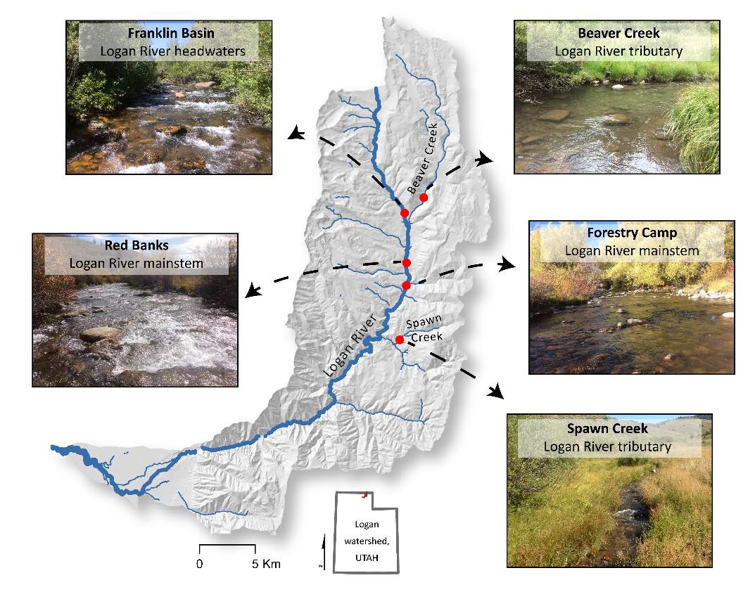
Figure 1. The study sites are located within the Logan River watershed and are either located on the mainstem Logan River or are tributaries to the Logan River.
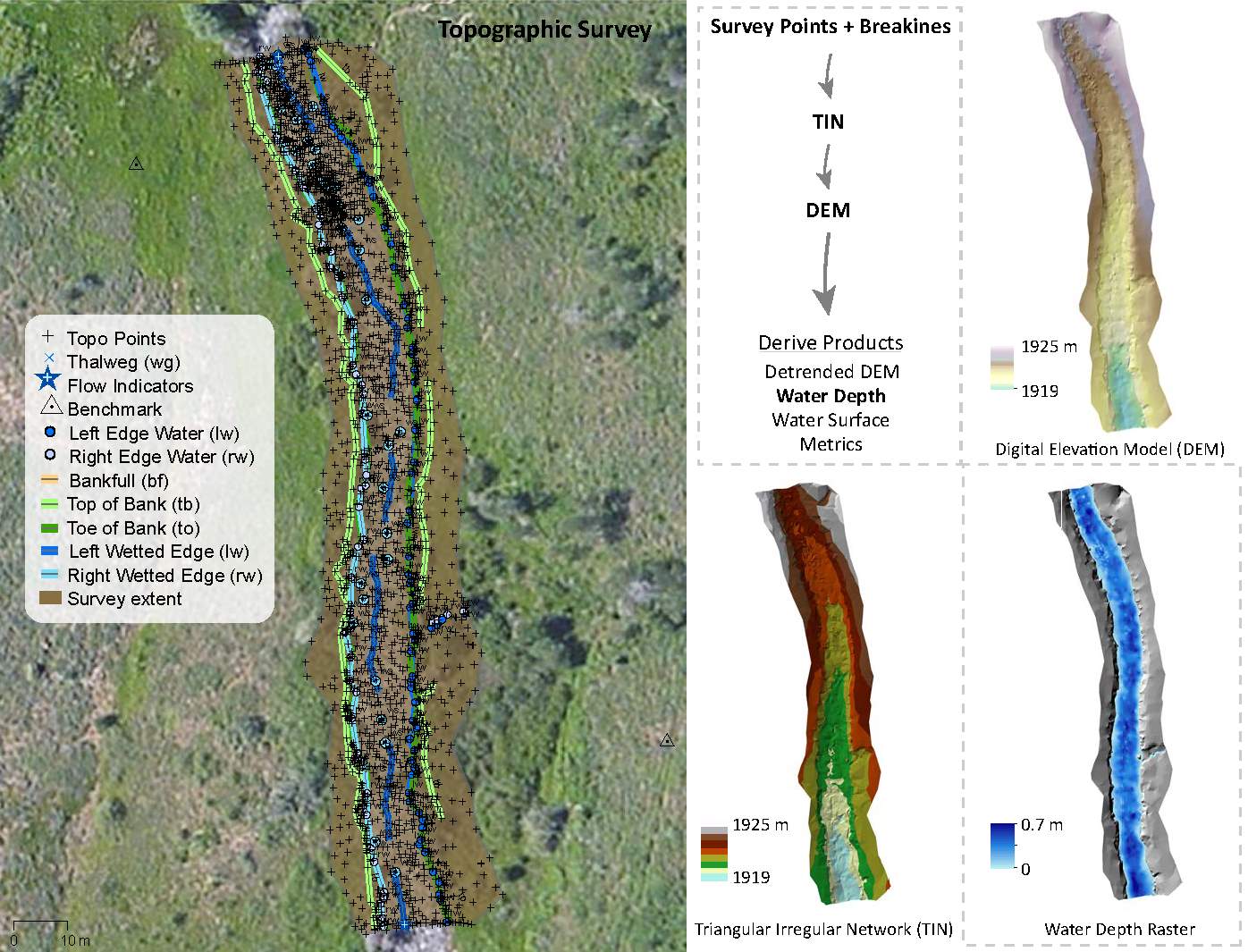
Figure 2. Topographic surveys were collected at each site and converted in digital elevation models, water surface and water depth rasters. Topographic derivates were used as inputs into the hydraulic model.
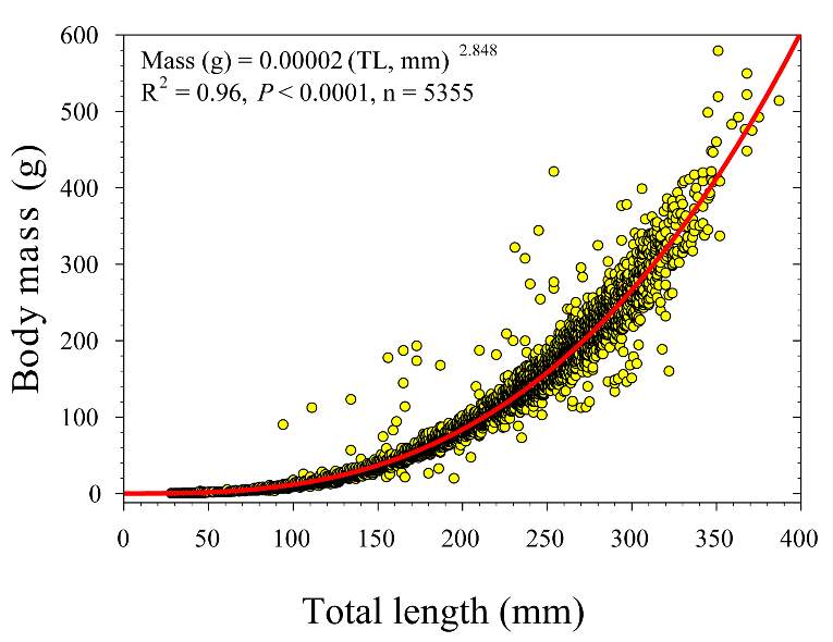
Figure 3. Length-to-weight (body mass) relationship for BCT in the Logan River, Utah from 2001-2015. Data from Budy (unpublished).
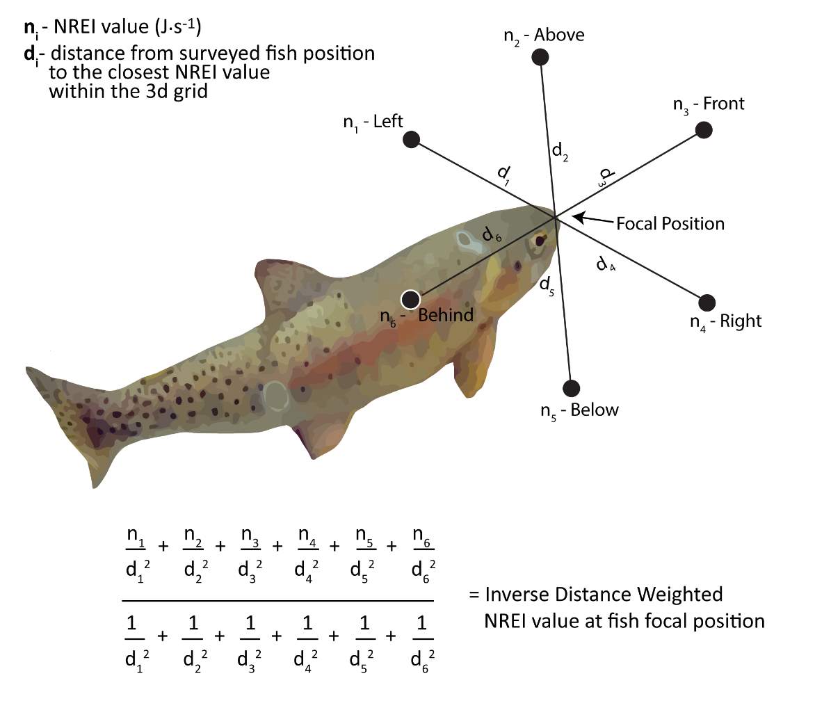
Figure 4. Inverse distance weighting was applied to each of the 6 nearest NREI estimates to identify the NREI estimate at each surveyed fish focal positon.
Figure 5. The depth and velocity map of each study site at baseflow conditions. Velocity magnitude (m∙s-1) is being shown as the site standard deviation in the map, while numeric velocity magnitudes are shown in the histogram.
Figure 6. The velocity vs. depth distribution for each site.
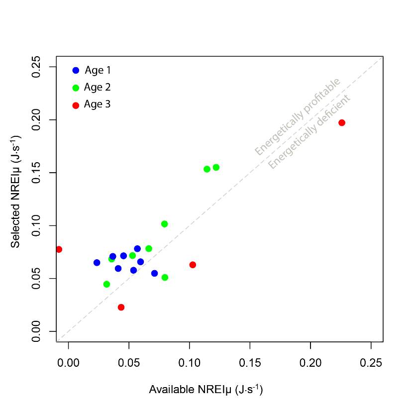
Figure 7. The relationship between the selected NREI mean, and the available NREI mean at each site, in each season, by age class. A line with a slope of 1 is shown for reference.
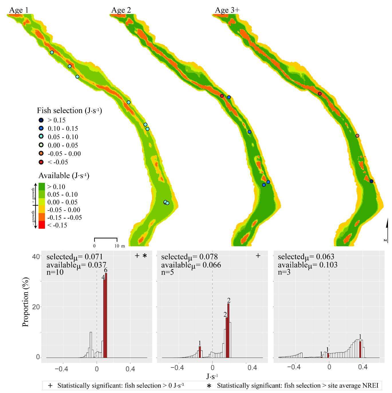
Figure 8. Red Banks, summer: used vs. available NREI distributions for each age class. The selected fish positions for each age class were mapped onto the depth-averaged NREI models of each site. a histogram was created which depicts the selected fish focal NREI estimate in red, and the available NREI distribution in white. In the histogram, the n value for each selected position is above the red bar.
Figure 9. Red Banks, fall: used vs. available NREI distributions for each age class. The selected fish positions for each age class were mapped onto the depth-averaged NREI models of each site. a histogram was created which depicts the selected fish focal NREI estimate in red, and the available NREI distribution in white. In the histogram, the n value for each selected position is above the red bar. Note the proportion axis in the historgram is different for age 1 fish.
Figure 10. Forestry Camp, summer: used vs. available NREI distributions for each age class. The selected fish positions for each age class were mapped onto the depth-averaged NREI models of each site. a histogram was created which depicts the selected fish focal NREI estimate in red, and the available NREI distribution in white. In the histogram, the n value for each selected position is above the red bar.
Figure 11. Forestry Camp, fall: used vs. available NREI distributions for each age class. The selected fish positions for each age class were mapped onto the depth-averaged NREI models of each site. a histogram was created which depicts the selected fish focal NREI estimate in red, and the available NREI distribution in white. In the histogram, the n value for each selected position is above the red bar.
Figure 12. Spawn Creek, summer: used vs. available NREI distributions for each age class. The selected fish positions for each age class were mapped onto the depth-averaged NREI models of each site. a histogram was created which depicts the selected fish focal NREI estimate in red, and the available NREI distribution in white. In the histogram, the n value for each selected position is above the red bar.
Figure 13. Spawn Creek, fall: used vs. available NREI distributions for each age class. The selected fish positions for each age class were mapped onto the depth-averaged NREI models of each site. a histogram was created which depicts the selected fish focal NREI estimate in red, and the available NREI distribution in white. In the histogram, the n value for each selected position is above the red bar.
Figure 14. Beaver Creek, summer: used vs. available NREI distributions for each age class. The selected fish positions for each age class were mapped onto the depth-averaged NREI models of each site. a histogram was created which depicts the selected fish focal NREI estimate in red, and the available NREI distribution in white. In the histogram, the n value for each selected position is above the red bar.
Figure 15. Franklin Basin, summer: used vs. available NREI distributions for each age class. The selected fish positions for each age class were mapped onto the depth-averaged NREI models of each site. a histogram was created which depicts the selected fish focal NREI estimate in red, and the available NREI distribution in white. In the histogram, the n value for each selected position is above the red bar.
Figure 16. The most abundant years of BCT at each site, since 2001.
Figure 17. Linear regression of maximum observed BCT density’s relationship (by mode fish size) with NREI-based carrying capacity. A 1:1 line is provided for reference.
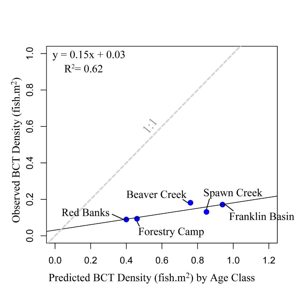
Figure 18. Linear regression of maximum observed BCT density’s relationship (by age class) with NREI-based carrying capacity. A 1:1 line is provided for reference.
Figure 19. Surveyed locations of Age 3+ cutthroat trout in October at the Forestry Camp site.
Figure 20. Depiction of a shear zone. Shear zones are found behind instream obstructions and provide energy refugia to salmonids. Shear zones are areas where fish can reduce swimming costs in the lower velocity water, but have access to the drifting insects in the higher velocity water, directly adjacent. Detecting shear zones in hydraulic model results requires that relevant flow obstructions are captured within survey topography.
Figure 21. Preliminary research on the mean energetic habitat quality within geomorphic units at Spawn Creek.
Figure A1. The recorded substrates within 1 meter of each fish, during snorkel surveys.
Figure A2. The mean NREI if all fish selected positions are averaged (by age class) and if fish found near boulders (potentially foraging in shear zones) are removed from the analysis at each site. The graph is divdied by season, site, and by age group of BCT.
Figure A3. The relationship between the mean NREI selected and the mean NREI available at each site. A) The relationship with all surveyed fish and B) the relationship if fish foraging near boulders are removed from the analysis. A line with a slope of 1 is shown for reference.
Figure_B1. The results of Geomorphic Unit Tool at Spawn Creek.
Figure_B2. The results of GUT at Red Banks, using a 55% capture rate and the drift and temperature at the time of snorkeling.
Figure_B3. The results of GUT at Forestry Camp using a 55% capture rate and the drift and temperature at the time of snorkeling.
Figure_B4. The results of GUT at Franklin Basin using a 55% capture rate and the drift and temperature at the time of snorkeling.
Figure_B5. The results of GUT at Beaver Creek using a 55% capture rate and the drift and temperature at the time of snorkeling.
Figure_B6. The distribution of NREI values within each geomorphic unit at Spawn Creek. The drift and temperature used were those collected during the snorkeling events: Drift 3.38 g.m3, temp 11.5° C.
Figure B7. The distribution of NREI values within each geomorphic unit at Red Banks. The drift and temperature used were those collected during the snorkeling events: Drift 1.65 g.m3, temp 11.4° C.
Figure B8. The distribution of NREI values within each geomorphic unit at Forestry Camp. The drift and temperature used were those collected during the snorkeling events: Drift 1.77 g.m3, temp 11.7° C.
Figure B9. The distribution of NREI values within each geomorphic unit at Franklin Basin. The drift and temperature used were those collected during the snorkeling events: Drift 1.5 g.m3, temp 9.0° C.
Figure B10. The distribution of NREI values within each geomorphic unit at Beaver Creek. The drift and temperature used were those collected during the snorkeling events: Drift 3.38 g.m3, temp 10.29° C.
Chapter 1
1.1 Introduction
A robust, quantitative understanding of fish-habitat relationships is essential to the effective conservation and management of fish populations. Worldwide, native salmonid populations have dramatically declined in abundance, distribution, and density over the last century with some populations impending extinction (Katz et al. 2013). In order to better understand and manage these fish populations, managers need information on specific habitat requirements. Habitat requirements are best described through a combination of biotic and abiotic characteristics, which influence fitness and survival of individual fish (Rosenfeld 2003). Traditionally, however, stream fish research has focused on the abiotic characteristics of sites (Wurtsbaugh et al. 2014), often overlooking biotic contributions to habitat suitability, such as the availability of prey or the presence and abundance of competitors or predators. Researchers are increasingly recognizing that physical habitat structure alone does not necessarily reflect the fish abundance or biomass a site can support (Naiman et al. 2012). Therefore, evidence is mounting that habitat should be evaluated in terms of both physical characteristics and food availability (Naiman et al. 2012).
Bioenergetics models offer a way to combine the both the biotic and abiotic characteristics of streams into one currency (i.e. energetic value) of habitat selection and habitat quality. These models are rooted in concepts of optimal foraging theory that assume natural selection favors individuals who respond to conditions within their environment when making foraging decisions in order to maximize their the Net Rate of Energy Intake (NREI) (MacArthur and Pianka 1966, Smith et al. 1983). Embedded in this assumption is the logic that if an individual fish maximizes its NREI on a daily basis, its chance of growth, survival and reproduction success will be maximized. These concepts have been applied to models of drift-foraging salmonid bioenergetics, with the basic premise that the energy available for growth (i.e. NREI) is equivalent to the energy gained from food, less the energy costs associated with metabolic processes (Fausch 1984, Hayes et al. 2000, Hughes et al. 2003). For stream-dwelling salmonids, this means that fish must capture and consume enough prey (a function of drift density, hydraulics, behavior) to offset the costs of existing at a particular location (a function of swimming costs, temperature, individual traits) in order to maintain positive growth. Bioenergetics models have successfully simulated the microhabitat selection of fish in the laboratory (e.g. Fausch 1984) and in the field (e.g. Guensch et al. 2001, Kotera and Inoue 2015). This approach has also been used to predict fish abundance (e.g. Urabe et al. 2010), biomass (e.g. Wall et al. 2015), carrying capacity (e.g. Hayes et al. 2007, Wall et al. 2015), and habitat quality (e.g. Jenkins and Keeley 2010, Urabe et al. 2010, Hafs et al. 2014).
Drift-foraging, bioenergetics models are increasingly being used to evaluate habitat quality and quantity, as well as carrying capacity of stream reaches (e.g., Hayes et al. 2007, Wall et al. 2015). However, many of these bioenergetics models have been developed and applied for salmonids at sites whose populations are well below carrying capacity (e.g., Wall et al. 2015). When fish populations are in low densities, comparative analysis could result in an underestimate of habitat potential and mask differences in use of different habitat types (Nickelson et al. 1992). Therefore, there is a need to assess model predictions in streams where salmonids are abundant to (i) gauge differences between actual fish positions and modeled energetic habitat predictions and (ii) the differences between observed densities and simulated carrying capacities.
To address these concerns, the objective of my thesis research was to test whether the Wall et al. (2015) NREI model could accurately predict the spatially-explicit foraging selection of Bonneville cutthroat trout (BCT; Oncorhynchus clarkiiutah) within the Logan River, Utah, a stream where one of the most abundant and well distributed populations of BCT reside (Teuscher and Capurso 2007). In addition to having an abundant and well-distributed population of BCT, the Logan River has minor anthropogenic disturbance, an intact riparian corridor, and has over 15 years of long-term BCT population data (e.g., Budy et al. 2007). Since populations of trout fluctuate over time (Platts and Nelson 1988), it is essential to have long-term BCT abundance data to compare to NREI model carrying capacity predictions. Further, Ideal free distribution theory (Fretwell 1972) assumes that, in an environment containing patches of differing habitat suitability, organisms will be aware of the resources available and will distribute themselves proportionally to take advantage of the available resources. In terms of NREI, organisms (i.e. the fish) should distribute themselves in terms of the energetic quality of the habitats available. Assuming this is true, the Logan River is an ideal location to test whether in a reach, possibly at carrying capacity, fish are disproportionality using the energetically favorable habitats (i.e. patches) in comparison to the other habitats available. In this research, I applied the bioenergetics model in two separate applications. The first application, in Chapter 2, examines whether the drift-foraging bioenergetics model can accurately predict the microhabitat foraging selection of BCT. The second application, in Chapter 2, addresses whether the NREI-based models predictions of carrying capacity are related to observed sample densities of BCT. In Chapter 3, I give ideas for future, related research questions. Finally, in Appendix A, I explore whether fish are potentially using instream topographic complexities which are not being captured by the hydraulic model and in Appendix B, I present preliminary research on whether instream geomorphic units have a characteristic bioenergetic signature.
Chapter 2
2.1 Introduction
Widespread habitat degradation (Lohn 2008) and fragmentation (Gregory and Bisson 1997) has significantly altered the distribution and abundance of salmonids across the Western United States (NOAA 2012). To effectively recover and/or conserve these fish populations, managers need tools that evaluate fish habitat quality in physically diverse streams and watersheds. Numerous studies have identified important characteristics of habitat quality, herein inferred to be equivalent to the fitness benefit of the habitat (e.g., Rosenfeld 2003), by quantifying empirical relationships between habitat features or by using physical habitat models to assess fish preference or abundance. While correlations between multiple physical stream attributes (i.e. dominant substrate, cover, % pools) and fish occupancy (e.g. Anlauf-Dunn et al. 2014), abundance (e.g. Smith and Kraft 2005, Smokorowski and Pratt 2007), or density (e.g. Roper et al. 1994, Roni and Quinn 2001) are sometimes used, the differing physical attributes between study sites makes their transferability questionable to other streams. Similarly, physical habitat models, such as PHABISM (Bovee 1986), combine abiotic stream habitat factors (typically depth, velocity, and substrate) to predict life stage and species-specific habitat suitability criteria and indices (HSI). These types of models are based on the frequency of use of physical habitats (Rosenfeld et al. 2005) and were developed by combining empirical studies and/or expert opinion (e.g. Raleigh et al. 1986). Although these models are sometimes used, research has shown that salmonids shift their habitat use in response to food availability (e.g., Rosenfeld et al. 2005), indicating that habitat selection based solely on physical variables can be misleading.
Bioenergetics fish habitat models (e.g., Hughes and Dill 1990, Hayes et al. 2000, Hayes et al. 2007, Wall 2014) offer an alternative mechanistic approach, combining both the physical habitat variables with the food availability into one measure of habitat quality. Bioenergetics models predict the position choice of individual fish in a stream based on a cost and benefit analysis of maximizing Net Rate of Energy Intake (NREI), while minimizing swimming costs (Fausch 1984, Hughes and Dill 1990, Addley 1993, Guensch et al. 2001). By combining swimming costs, reaction distances, local hydraulics, and energy (in the form of drifting insects), these models have been shown to predict feeding position choice by a variety of drift feeding salmonids (e.g., Hughes and Dill 1990, Addley 1993, Hayes et al. 2000, Guensch et al. 2001, Hughes et al. 2003). Bioenergetics models have been used to characterize site selection (e.g., Hayes et al. 2007) and determine habitat quality (e.g., Jenkins and Keeley 2010, Urabe et al. 2010), in addition to patterns of growth (e.g., Rosenfeld and Boss 2001). Hayes et al. (2007) extended the NREI modeling framework, linking a hydraulic model with drift dispersion and bioenergetics foraging processes. This innovative approach allowed for bioenergetics testing over a range of flows, allowing for extension of the model into new applications. Recently, Wall et al. (2015), using an adaption of the Hayes model, applied the NREI modeling framework to monitoring and management (Rosenfeld and Tonn 2014) and found positive correlations between the models’ predicted carrying capacities and imperiled steelhead salmon densities in 22 study sites within the Columbia River Basin.
Despite the increase in the use of NREI-type models (Hayes et al. 2007, Jenkins and Keeley 2010, Kotera and Inoue 2015, Wall et al. 2015), these models have been only been assessed for a limited number of species, casting potential doubts over their applicability to species other than which they have been assessed (Chipps and Wahl 2008). For example, model parameters are often borrowed from related species when swimming costs and other physiological parameters are not available for the species of interest. Although borrowing parameters is common (e.g., Hayes et al. 2007, Urabe et al. 2010, Kotera and Inoue 2015), the borrowed values need to be tested to determine if they are applicable to the species of interest. In addition, many fish populations are not at carrying capacity. When fish populations are in low densities, comparative analyses could result in an underestimate of habitat potential and mask differences in the use of different habitat types (Nickelson et al. 1992). Therefore, these simulated carrying capacities need to be tested in streams that are thought to have high abundances of the species of interest.
In light of these uncertainties, I sought to improve the current understanding on the use of NREI models for differentiating within-reach bioenergetics habitats and carrying capacity predictions of drift-feeding salmonids, using Bonneville cutthroat trout (BCT; Oncorhynchus clarkiiutah) in the Logan River as my test species. Bonneville cutthroat trout are limited to the Bonneville Basin of the Interior United States (Hepworth et al. 1997) and are the only trout species that is endemic to the basin. In the mid-century, the BCT was thought to be extinct throughout the Basin, however, conservation and stocking programs have successfully restored BCT to some of their natal streams (Behnke 2010). In 2000, to prevent the listing of BCT by federal or state agencies, a Conservation Agreement was formed between the Utah Department of Natural Resources, Idaho Fish and Game Department, Nevada Division of Wildlife, Wyoming Game and Fish Department, Confederated Tribes of the Goshute Reservation, and the United States Department of the Interior (Lentsch et al. 2000). The interagency agreement enacted a series of conservation and land management plans to address habitat loss (Hilderbrand and Kershner 2000), habitat degradation (e.g. Budy et al. 2003), hybridization (USDOI 2001), and competition with non-native species (McHugh and Budy 2005). As a result, three out of the fourteen listed conservation strategies are to 1) Describe the BCT habitat requirements, 2) To enhance and maintain habitat, and 3) To monitor habitat quantity and quality (Lentsch et al. 2000). Therefore, the NREI model, if proved useful for BCT, could be used as a way to address these habitat concerns.
The intent of my research is to determine if bioenergetics models are a useful tool for identifying the quality and carrying capacity of salmonid trout habitats in a system with an abundant population of salmonids. These models have potential to inform managers on how changes in stream temperature (i.e. climate change) or water withdrawals could affect trout, both of which are problems that will affect the western United States over the next century. However, many of the places in which bioenergetics models have been run are for threatened species occupying habitats at densities well below carrying capacity. Therefore, my objective is to assess the applicability of the drift-foraging bioenergetics model by assessing model predictions of the focal foraging positions and carrying capacity of fish in a system nearer to carrying capacity – i.e. BCT in the Logan River. Since, the BCT population in the Logan River is one of the most dense populations (per stream km) of inland cutthroat trout (Budy et al. 2007) and one of the most well-distributed (Teuscher and Capurso 2007) populations of BCT, it is an ideal location to test the bioenergetics model carrying capacity predictions and BCT focal foraging positions. The specific questions my research will address are: 1) Do BCT use focal foraging positions consistent with NREI model predictions of energetic suitability? 2) Is the use consistent across varying temperatures, discharges, and drift values? 3) Does the NREI model predicted carrying capacity relate to the observed density of BCT in the Logan River?
2.2 Methods
2.2.1 Study Site – Logan River and Logan River tributaries
The Logan River is located in Southeastern Idaho and Northern Utah, flows in a southwestern direction and is a tributary to the Bear River. The uppermost river reaches flow through partly confined valleys surrounded by formerly glaciated peaks (iUtah 2015), the middle reaches flow through a confined canyon, and the lowermost reaches flow through an open unconfined broad valley before it joins the Bear River. The Logan River is the largest water contributor to the Bear River watershed, which terminates at the Great Salt Lake. At the headwaters of the Logan River, in Franklin Basin, air temperature ranges from -22° C to 30° C, while river temperatures range from 0° C to 12° C (iUtah 2015). Most of the annual precipitation (43 to 150 cm) occurs as snow, yielding a snowmelt-driven hydrology with peak runoff of 16 m3⋅s−1 in late spring and baseflow conditions of 3 m3⋅s−1 the rest of the year (USGS 2001). The river is a cold water fishery providing critical habitat for BCT, a ‘conservation’ species in the states of Utah and Idaho. The river also supports populations of brown trout (Salmo trutta), rainbow trout (Oncorhynchus mykiss), brook trout (Salvelinus fontinalis), mountain whitefish (Prosopium williamsoni), and mottled sculpin (Cottus bairdi) (Budy et al. 2014). The riparian habitat is dominated by grasses/forbs, willow (Salix spp.), chokecherry (Prunus spp.), elderberry (Sambucus spp.), Boxelder (Acer spp.) and Aspen (Populus spp.).
I chose five study reaches in the Logan River watershed to study the focal positions selected by BCT, the available energetic potential, and the carrying capacity, as predicted by the NREI model. The study reaches were selected based on the location of existing instream HOBO data loggers and 16 years of long-term monitoring (e.g., Budy et al. 2003, McHugh et al. 2008, Randall 2012, Budy et al. 2014, Mohn 2016), which includes electrofishing-based population surveys by the USGS Utah Cooperative Fish and Wildlife Research Unit. Of the 8 long-term index sites, surveyed annually by the USGS Utah Cooperative Fish and Wildlife Research Unit, I chose to study the five highest elevation reaches because they are dominated by BCT, whereas the lower reaches have brown trout, a competitor, and rainbow trout, which affects BCT negatively through hybridization (Budy et al. 2014, Meredith et al. 2016). The sites represent a variety of valley confinement types (see Brierley and Fryirs 2013), valley and bankfull widths, stream slopes, stream orders and the amount of upstream drainage area all of which can affect the local hydraulics (i.e. depth, velocity, water temperature) of the stream and ultimatetly the NREI model output. Site characterisitcs are shown in Table 1 and the sites are depicted in Figure 1.
Table 1. General site characteristics. The dominant vegetation at each site is a mixture of sagebrush, willow, dogwood, and grasses/forbs.
| Site | Valley confinement | Avg. valley width (m) | Avg. bankful channel width (m) | Stream slope range (%) | Strahler stream order | Upstream drainage area (sq. km) |
| Red Banks | Partly Confined | 39 | 12.5 | 2-7 | 4 | 296 |
| Forestry Camp | Unconfined | 86 | 13 | 1-5 | 4 | 359 |
| Franklin Basin | Partly Confined | 20 | 9.5 | 4-11 | 3 | 108 |
| Beaver Creek | Partly Confined | 22 | 7 | 4-7 | 3 | 129 |
| Spawn Creek | Unconfined | 18 | 2.4 | 4-10 | 2 | 17 |
Figure 1. The study sites are located within the Logan River watershed and are either located on the mainstem Logan River or are tributaries to the Logan River.
2.2.2 Habitat Data Collection and Processing
2.2.2.1 Habitat Surveys
Topographic and habitat surveys were collected during baseflow conditions at the five study sites in August and September 2015. Five stream reaches were surveyed using a combination of total stations (TS) and real-time kinematic (rtk) GPS using the protocol developed for the Columbia Habitat Monitoring Program (CHaMP) (Bouwes et al. 2011, CHaMP 2015). The CHaMP topographic survey protocol was designed to capture the stream and floodplain features that define fish habitat, specifically: topographic breaklines, stream geomorphology, and topographic features that steer and route the streamflow, giving rise to local hydraulics (Wheaton et al. 2004). Using a topographically stratified approach, I collected denser points near breaks in slope and topographically complex areas, and lower point densities in topographically homogeneous areas (Bangen et al. 2014). The topographic surveys were tied to real-world coordinates through rtkGPS surveys and processed into digital elevation models (DEMs) in ArcGIS, release 10.1 (ESRI 2014), to build a three dimensional, continuous representation of the stream topography using the CHaMP Topo Processing Tools Version 5.0.11.0 (http://champtools.northarrowresearch.com). Once the DEM was created, the CHaMP Topo Toolbar was subsequently used to create water depth and water surface rasters (Figure 2). The water depth raster is used as an independent validation of the hydraulic model depth output, whereas points are sampled from the water surface raster and are used for the downstream water elevation in the hydraulic model.
Figure 2. Topographic surveys were collected at each site and converted in digital elevation models, water surface and water depth rasters. Topographic derivates were used as inputs into the hydraulic model.
I collected and quantified three additional physical habitat variables for bioenergetics modeling: substrate roughness, discharge, and temperature. Substrate roughness was estimated based on pebble counts. More specifically, 110 particles were measured within each site, spread across 11 evenly spaced transects. Substrate roughness was estimated as the 84th percentile (D84 hereafter) of the cumulative size frequency distribution of the pebbles and used as the height parameter in the hydraulic model (ISEMP/CHaMP 2015). I measured discharge by taking depth and velocity measurements at a uniform cross section (Peck et al. 2001, CHaMP 2015), divided into 15-20 equally spaced intervals that were at least 10 cm wide. A Marsh-Mcbirney Model 2000 Flo-mate (Marsh-Mcbirney Inc., Maryland, USA) was used to record velocity at 60% of the depth from the water surface, while a depth rod was used to record the depth at every interval. The product of depth, velocity, and station width (i.e. >10 cm) were then summed to obtain an estimate of discharge at the top of the site. To calculate discharge during snorkeling events, which occurred on a different day, I developed calibration relationships using site measurements and the daily discharge readings at the Forestry Camp iUtah gage site (iUTAH 2016). A ratio was used to extrapolate the discharge, rather than a regression because of the small sample size (n=10) (see Rosenfeld et al. 2016). Stream temperatures were calculated for the 7 day average prior to snorkeling from in-stream temperature HOBO (Onset Computer Corporation, Massachussetts, USA) logger data (Budy, unpublished data).
2.2.2.2 Invertebrate Drift
Field: During snorkel surveys, I collected drifting prey items (a key input to NREI) at each site by deploying two side by side mesh driftnets (20 x 20 cm opening, 500 µm mesh) at the upstream end of each site. All nets were placed on 2 cm spacers, holding the net above the river bottom to prevent benthic invertebrate capture and deployed in depths that ranged from 10 cm to 40 cm, in areas with a relatively uniform flow. To estimate the volume of water sampled, I measured current velocity at 60% depth and total water depth within the net, at the start and end of sampling. I preserved each sample in 90% ethanol in the field for later analysis in the laboratory.
Laboratory: Consumption of prey is limited by salmonid gape size, foraging cost and benefit, and gill raker spacing (Wankowski 1979). Based on these requirements, the minimum prey length a 100 mm salmonid will consume is >1 mm (e.g., Wankowski 1979). Therefore, I selected all macroinvertebrates >1 mm from the preserved material. Once all macroinvertabrates >1mm were selected, at least 45 specimens from each site were measured to the nearest 0.2 mm to obtain an average site prey length, a necessary input into the NREI model. All of the macroinvertebrates >1mm were then rinsed in de-ionized water and dried at 105° C for 48 hours until they reached a stable weight . After being dried, the samples were weighed to the nearest 0.1 milligram to obtain an ash-free dry biomass (Hauer and Lamberti 2011).
To use these data in the NREI model, which assesses foraging in terms of individual prey items, dry weight was converted to a measure of invertebrate abundance per cubic meter. First, the volume of water filtered in each net was calculated by:
Average net depth (m) x net width (m) x average net mouth velocity (m·s-1) x sampling duration (s)
The average net depth and net mouth velocity were calculated by averaging the initial depth and velocity, taken at the beginning of the sample, with the depth and velocity taken at the end of sampling. Once the volume of water filtered was calculated for each net, it was then summed for a total volume of water filtered during the sample duration. The total volume of water was then divided by the total sample dry weight. The resulting value was divided by the average dry weight of a ‘typical’ prey item for each site, which was assumed be a mayfly with a length equivalent to site-average prey length (Smock 1980). This calculation resulted in the average number of mayflies per cubic meter of water at each site, during the time of snorkeling.
2.2.2.3 Snorkel surveys
BCT microhabitat snorkel surveys were conducted during the summer and fall of 2015. Snorkel surveys have been employed extensively in fisheries because they are a useful, noninvasive, and inexpensive way to identify habitat use by species (Roper et al. 1994, O’Neal 2007, Weaver et al. 2014). Depending on the size of the wetted width of the stream, one or two snorkelers surveyed the stream segment, working upstream in a zig-zag pattern, visually identifying fish locations. Snorkelers inspected all visible portions of the wetted channel for fish. Once a fish was located, snorkelers recorded the species, total length, depth in the water column, the substrate within a 1 m diameter of the fish location, and the behavior. The focal depth of the fish was recorded in one of four categories, starting at the bottom of the stream: the lowest 25% of the water column, 25-50% of the water column, 50-75% of the water column, or the top 75-100% of the water column (Al-Chokhachy and Budy 2007). The behavior of the fish was recorded so that I could quantify whether the fish was foraging, moving, or holding a resting position. Only fish >100 mm, age-1 or older (Meredith et al. 2014), were surveyed. Snorkelers placed a numbered washer at each fish’s location so that a survey technician could get a precise GPS location (rtk or TS).
All surveys were conducted during baseflow conditions from August 5 – 13, and repeated at three sites (Spawn Creek, Forestry Camp, and Red Banks) from October 8- 15. The snorkel surveys were conducted during the middle of the day when stream temperatures were between 10° C and 18° C when fish are known to actively forage, as recommended in the Salmonid Field Protocols Handbook (O’Neal 2007).
2.2.2.4 Long-term fish collections
Using short term studies to assess fish abundance over time can be problematic since some cutthroat trout populations in the Great Basin have exhibited large annual fluctuations (Platts and Nelson 1988) and, wild cutthroat trout have exhibited substantial yearly variation even when conditions remained the same (House 1995). Therefore, to assess abundance of BCT in the Logan River, I used a data set that the USGS Utah Cooperative Fish and Wildlife Research Unit has estimated abundance every year since 2001, at each of my study sites. To estimate fish abundance, the USGS Utah Cooperative Fish and Wildlife Research Unit uses a three-pass depletion technique during low flow conditions. They use a backpack- or canoe-mounted electrofishing unit which varies in voltage depending on the stream conditions (300 – 400 μS/cm, 8 – 15 oC, 40-Hz pulsed DC, 160 – 500 volts, 0.2 – 4 amps) to shock the fish. They anesthetize the fish, count them, and measure their length and weight before returning them to the stream (Budy et al. 2014). See Budy et al. (2007) for a more detailed description of the long-term population monitoring in the Logan River.
2.2.3 NREI Modeling
2.2.3.1 Spatially explicit NREI predictions
To test whether the NREI model can accurately predict the microhabitat foraging selection of BCT, each site had a site-specific bioenergetics model built by combining multiple data sources that reflect the foraging ecology and energetic requirements of salmonids. I used physical habitat characteristics (i.e. depth, velocity) of each site to model hydraulics, and calculated average stream temperatures, drift densities and prey sizes for the foraging and swimming cost models. Since fish physiological traits are size and weight dependent (Jobling 1995), I used observed length and calculated the estimated weight with a BCT-specific length –weight regression (Mass (g) = 0.00002 (Total Length (mm))2.848) developed from 2001-2015 Logan River electrofishing data (Budy, unpublished, Figure 3). Observed fish were then grouped into an age classes (e.g., Budy et al. 2007) based on the length of the fish: 100-149 mm fish were classified as Age 1, 150-224 mm fish were classified as Age 2, and 225 mm fish and larger were classified as Age 3+. The NREI model was run separately for each size class. Thus, the broader NREI landscape considered for available positions and used positions (described below) changes within each size-specific analysis. I assumed a 55% foraging success rate (Hughes et al. 2003, Wall et al. 2015) for the foraging submodel, and I also assumed a uniform drift density for model simplicity (Wall et al. 2015). For swim cost calculations, I assumed that steelhead and BCT have similar swimming costs, since they are a sympatric species and since cutthroat specific swimming costs have not been parameterized.
Figure 3. Length-to-weight (body mass) relationship for BCT in the Logan River, Utah from 2001-2015. Data from Budy (unpublished).
To model stream hydraulics, a hydraulic model was built for each site by using the coordinates (x,y,z) of the DEM nodes, discharge measurements, substrate roughness, and water surface elevations derived from the processed topographic surveys (cf. Wall 2014). Site discharge measurements were used as the upstream hydraulic boundary and the topographically derived water surface elevations were used as the downstream boundary. During modeling, it was assumed that water was not lost or gained in the reach. Flow patterns were modeled using a depth-averaged two-dimensional mode (i.e. produces 2D flow vectors of velocity at every computational node) of the Delft3d hydraulic modeling software (Delft 2016). The hydraulic modeling output was used to create a 3d grid of wetted points, and then converted to a depth-averaged velocity output. The depth-averaged velocity output, produced for this research, is a 2.5d representation of the stream’s velocity since the model assumes a logarithmic velocity profile throughout the water column. The output of the hydraulic modeling process was a 3d grid of the depths and velocity (scalars) that were used as an input into the foraging and swimming cost models.
NREI was computed by combining hydraulics with multiple characteristics that would affect the efficiency of both foraging and swimming. I used an adaptation of the NREI framework developed by Wall et al. (2015). Briefly, at each potential foraging location (i.e., a point within the 3d grid), the foraging model predicted the gross rate of energy intake (GREI) from invertebrate drift concentration and average prey size, height of foraging above the streambed, temperature, fish length, and local hydraulics. Swimming costs were then estimated for the same point as a function of stream temperature, velocity at the focal point, and fish weight. The foraging area of a single fish was modeled by delineating 36 equally-spaced radials emanating from the fish’s focal position, as if the fish was looking upstream with the ability to capture prey in multiple 3d directions: above, below, to the right, or to the left. Each radial had 1 cm spaced nodes; at each node, drift concentrations were set to the reach average value and velocities were interpolated from nearby 3d grid points. Each node, on each radial, was evaluated to see if a fish could theoretically swim fast enough to capture prey items or if the prey items would be swept downstream before the fish could intercept them. The GREI estimates at individual nodes were summed to estimate total GREI for the focal point, which was then reduced by 30% to account for waste (Hughes et al. 2003). The resulting NREI was calculated by subtracting the metabolic cost of swimming from the adjusted GREI to predict the energetic profitability of each location within the stream ((GREI X 0.7)-swimming cost=NREI).
To estimate the NREI for locations that BCT were observed to use during snorkel surveys, all NREI 3d point data were divided into selected (i.e. used) and available (i.e. unused) positions for analysis. I used individual age class of fish, along with the observed depth, modeled velocity, site temperature (prior 7-d mean), and drift abundance to estimate the energy available for each of the surveyed fish at each of the study sites. The selected fish position NREI value was computed by taking the inverse distance weighted mean of the 6 closest NREI values in 3d space (Figure 4).
Figure 4. Inverse distance weighting was applied to each of the 6 nearest NREI estimates to identify the NREI estimate at each surveyed fish focal positon.
2.2.3.2 NREI predictions of site carrying capacity
In addition to spatially explicit predictions of NREI, model output can be used to estimate the carrying capacity of each study site, based on food availability and habitat characteristics of each site. To do this, the model requires two additional inputs: 1) a minimum NREI threshold value, above which an assessment point within the 3d grid is assumed to be ‘usable’, and 2) an estimate of territory size, taken as the area surrounding a (potential) fish’s location which is no longer available for occupancy by other individuals. For this research, the threshold value of 0.0 J·s-1 was chosen because this is the threshold at which fish are projected to neither gain nor lose weight (Wall et al. 2015). Fish territories were calculated from an allometric body size–territory size relationship (Imre et al. 2004), then multiplied by 2 to ensure that fish territories don’t overlap. To predict carrying capacity, a fish placement algorithm is used. Beginning with the highest NREI value in the study site, a fish is placed and all points within the fish’s territory are deemed no longer available. This process is then repeated at the next-highest NREI value until no more usable positions remain. This process results in a carrying capacity estimate of each reach (i.e. estimated fish count the reach can support). However, since observed counts of BCT are collected at sites that vary in wetted width each year (which affects total area), I converted both the observed fish counts and model-simulated carrying capacity to an estimate of density (fish·m-2) by dividing the total fish by the area of the reach (square meters), to allow for both site and yearly comparisons. The model requires a fish size input to predict capacity (i.e. the model simulates capacity of each age class separately), therefore, I chose to use the most common size (i.e. mode) of fish observed while snorkeling. All NREI model analysis was completed in R software, version 3.3.1 (R Core Team 2016).
At each study site, the observed fish density (fish·m-2) or biomass (g·m-2) was compared to three NREI model derivatives that have been used by previous researchers. First, I compared the observed fish density to the predicted carrying capacity for the most common fish size (i.e. mode) at the reach. Wall et al. (2015) found observed and predicted capacity to be positively correlated in 22 study sites of the Columbia River Basin, thus this metric was used to indicate whether the model worked for BCT. The second metric I computed was whether the proportion of suitable locations (the quotient of all locations with NREI > 0.0 J·s-1 and the total number of NREI estimates at the study site) was correlated to the observed BCT density. Last of all, I calculated the mean NREI and compared this value to the observed biomass at each study site. Biomass was calculated by multiplying the weight (g) of the fish, calculated from the length-weight regression formula (Budy, unpublished; Figure 3) to the observed abundance of fish at that site. The calculated biomass was divided by the size of the site (m-2), to obtain a biomass per area. All three metrics were previously computed by Wall et al. (2015) and Urabe et al. (2010) to compare NREI model estimates to steelhead (Oncorhynchus mykiss) and masu salmon (Oncorhynchus masou) densities and biomass, respectively.
2.2.4 Statistical Analyses
Using NREI estimates for selected and available locations, I assessed whether the potential foraging positions used by BCT were suitable for growth (H1: NREI-used > 0.0 J·s-1) and whether BCT preferentially used the most profitable locations within sites (H1: NREI-used > NREI-available) using a combination of parametric and nonparametric statistical tests. A two way between subject ANOVA was used to test if there was a difference between the three levels of behaviors: foraging, holding, or moving. Before further analysis, I wanted to know if the fish behavior warranted separate analyses since the NREI model is specific to foraging. Based on an exploratory analysis of the relationship between the selected NREI value and the three behaviors, I found there was no evidence of differences in the selected energetic value between the three behaviors during summer or fall, at any of the sites, or for any of the age classes. Therefore, behavior was not included in the analyses. To determine if there was any evidence that fish were maintaining focal positions that were energetically profitable, for each site, season, and age class, I used a Student’s t-test to calculate whether the position that the fish was selecting was greater than 0.0 J·s-1. While the selected fish points were normally distributed, the available NREI distributions for each site were not. Therefore, I used non-parametric one-sided Mann Whitney U-tests, to determine if the median of selected NREI distributions was greater than the median of available NREI distributions. The available NREI points at each site far surpass the selected points at each site (n~250,000 available points at each site, n=9-63 selected points). To mitigate for the unbalanced distributions, 200 randomly sampled points were selected from the available NREI distributions. A Mann-Whitney test statistic was computed 10,000 times on the selected and randomly sampled available distributions, and averaged. Finally, I conducted linear regression to examine whether observed densities of BCT were related to NREI predicted carrying capacity or proportion of suitable habitat and to assess whether fish biomass (g.m2) was related to mean NREI. All tests were assessed for statistical significance at = 0.10.
2.3 Results
2.3.1 Overview of survey dataset
Snorkel surveys were collected at five streams during the summer of 2015, and three sites were re-visited in the fall of 2015. The mean water depth ranged from 0.13 – 0.29 m between the five sites and the mean velocity ranged from 0.12 to 0.3 m·s-1 (Figure 5 and Figure 6). Discharge, drift, and stream temperatures all declined between the summer and fall samples ( REF _Ref479162133 h Table 2Table 2 ). At the five sites, macroinvertebrate abundances varied by as much as 4x and discharge varied by up to 9x. A total of 216 cutthroat trout were observed in the Logan River: 128 fish were observed in summer (August), and 88 fish were observed in fall (October) (Table 3). The most common fish size observed in the summer was 125 mm, while the most common size observed in the fall was 150 mm.
Figure 5. The depth and velocity map of each study site at baseflow conditions. Velocity magnitude (m∙s-1) is being shown as the site standard deviation in the map, while numeric velocity magnitudes are shown in the histogram.
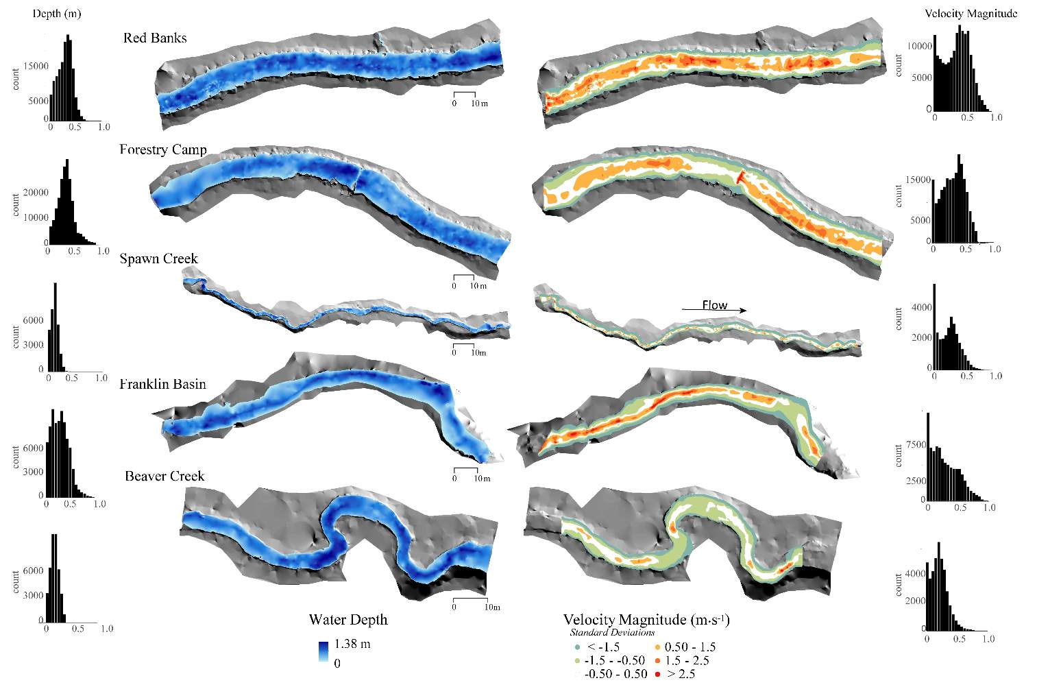
Figure 6. The velocity vs. depth distribution for each site.
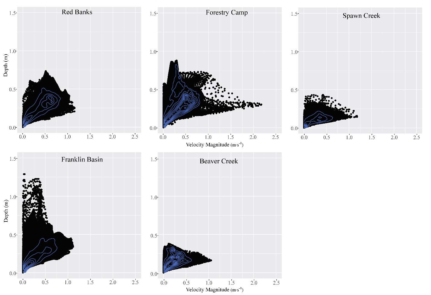
Table 2. General site characteristics and snorkel survey dates. The average 7 day temperature was calculated for the 7 days prior to each snorkeling event, the drift and discharge were calculated for the time of snorkeling. The upper part of the table shows the summer snorkel dates and site-specific NREI model inputs, while the lower portion of the table shows the same data for the fall snorkel events.
| Site | Site Length (m) | Snorkel date | Avg. 7 Day Temperature (°C) | Drift (g∙m-3) | Discharge (m3∙s-1) |
| Beaver Creek | 100 | 8/12/15 | 10.3 | 6.14 | 0.16 |
| Forestry Camp | 200 | 8/05/15 | 11.8 | 3.22 | 1.45 |
| Franklin Basin | 100 | 8/13/15 | 8.9 | 1.52 | 0.63 |
| Red Banks | 200 | 8/05/15 | 11.4 | 3.00 | 1.33 |
| Spawn Creek | 120 | 8/12/15 | 11.5 | 4.50 | 0.10 |
| Forestry Camp | 200 | 10/15/15 | 9.6 | 1.20 | 0.71 |
| Red Banks | 200 | 10/08/15 | 9.8 | 2.25 | 0.71 |
| Spawn Creek | 120 | 10/11/15 | 9.4 | 3.20 | 0.06 |
Table 3. BCT observed at each site
| Age class | Beaver Creek | Forestry Camp | Franklin Basin | Red Banks | Spawn Creek | n | ||
| summer | 1 | 8 | 6 | 10 | 23 | 7 | 54 | |
| 2 | 1 | 12 | 5 | 29 | 3 | 51 | ||
| 3 | 11 | 3 | 10 | 24 | ||||
| n summer | 9 | 29 | 18 | 62 | 10 | 128 | ||
| fall | 1 | 4 | 16 | 8 | 28 | |||
| 2 | 16 | 26 | 3 | 45 | ||||
| 3 | 9 | 6 | 15 | |||||
| n fall | na | 29 | na | 48 | 11 | 88 | ||
| Total | 9 | 58 | 18 | 110 | 21 | 216 |
2.3.2 Relationship between fish locations and NREI estimates
I examined whether the fish focal position was energetically profitable as a pooled sample (all sites and season), and for each site and season individually. In the pooled sampled, the majority (84%) of all individual fish, were choosing focal habitats where NREI estimates were greater than 0.0 J·s-1, a threshold above which fish are projected to grow. In addition, the mean NREI for fish selected positions was consistently higher than the mean available NREI estimate at each study site, in each season (Figure 7). This suggests that the majority of fish chose focal positions that maximized their NREI.
Figure 7. The relationship between the selected NREI mean, and the available NREI mean at each site, in each season, by age class. A line with a slope of 1 is shown for reference.
In the summer, 86 % of all Age 1 fish selected focal positions that provided NREI values sufficient for growth (>0.0 J·s-1) (Significant at all sites: Red Banks (t = 7.88, P t=7.82, P t=5.12, P=0.001), Beaver Creek (t=2.82, P=0.012) and Franklin Basin (t=64.85, P U=1594, P = 0.005), Franklin Basin (U=736, P=0.01); Not significant: Forestry Camp (U=688.77, P=0.23), Spawn Creek (U=790.88, P=0.28), Beaver Creek (U=711.32, P=0.70)). All (100%) of the Age 2 fish were selecting focal positions that provided enough energy for growth (significantly > 0.0 J·s-1 at Red Banks (t=3.75, P t=25.2, P t=1.66, P=0.09); Not significant: Spawn Creek (t=0.83, P=0.25), Beaver Creek (sample size too small for testing). The majority (63-100%) of Age 2 fish were also selecting focal positions that were higher than the site average (Not significant at Red Banks (U=3215.73, P=0.19, Forestry Camp (U=1266.9, P =0.38, Spawn Creek (U=241.31, P=0.72), Beaver Creek (sample size too small for testing), Franklin Basin (U=552.28, P=0.35)). Age 3 fish were only observed at Forestry Camp, Red Banks, and Franklin Basin. Of these fish, they were all (100%) selecting focal positions which would allow them to grow (Significantly >0.0 J·s-1 at Red Banks (t=1.67, P=0.06), and Forestry Camp (t=3.19, P=0.005), Not significant: Franklin Basin (t=0.61, P=0.30)). The majority of age 3 fish at Red Banks (80%) and Forestry Camp (73%) were choosing focal positions better than site average NREI estimate, however, only one out of the 3 fish surveyed at Franklin Basin used a focal position with an NREI value better than the site average (Significant: Red Banks (U=1060.03, P=0.07), Not significant: Forestry Camp (U=1075, P=0.55), Franklin Basin (U=251.18, P=0.69)).
In addition to summer, focal positions were surveyed at three of the five study sites during the fall: Red Banks, Forestry Camp, and Spawn Creek. At these sites, Age 1 fish were selecting focal positions that would allow them to grow at all sites (Significant all sites: Red Banks (t=5.67, P t=15.9, P t=14.09, P U=656, P=0.001), Not significant: Red Banks (U=1600.68, P=0.49). Age 2 fish were also selecting focal positions that would allow them to grow (Significant all sites: Red Banks (t=8.00, P t=6.68, P t=3.29, P=0.04)), and 67-81% were selecting focal positions with higher NREI than the site average (Significant at Red Banks (U=3270.52, P=0.02), Forestry Camp (U=2030.025, P=0.04); Not significant; Spawn Creek (U=347.56, P=0.33)). While 83% of age 3 fish at Red Banks were selecting focal positions with NREI estimated values above 0.0 J·s-1, conversely, all fish at Forestry Camp were selecting focal positions with negative NREI estimates (Not significant; Red Banks (t=0.41, P=0.35), Forestry Camp (t=-7.13, P=0.99). At Forestry Camp the mean selected position and the mean available NREI estimate were both less than 0.0 J·s-1. However, the majority of fish (67-100%) at Red Banks and Forestry camp were still selecting better than site average NREI estimate (Not significant: Red Banks (U=617.61, P=0.45), Forestry Camp (U=587.54, P=0.95). The selected fish positions for each age class were mapped onto the depth-averaged NREI models of each site (Figure 8, Figure 9,Figure 10,Figure 11,Figure 12,Figure 13,Figure 14,Figure 15).
Figure 8. Red Banks, summer: used vs. available NREI distributions for each age class. The selected fish positions for each age class were mapped onto the depth-averaged NREI models of each site. a histogram was created which depicts the selected fish focal NREI estimate in red, and the available NREI distribution in white. In the histogram, the n value for each selected position is above the red bar.
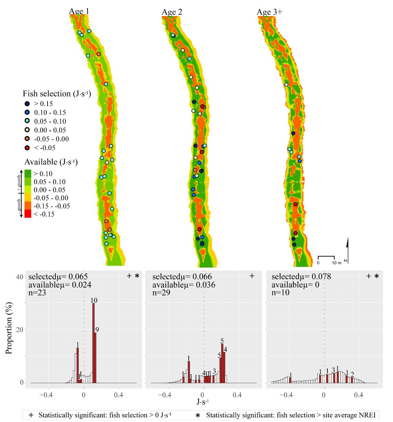
Figure 9. Red Banks, fall: used vs. available NREI distributions for each age class. The selected fish positions for each age class were mapped onto the depth-averaged NREI models of each site. a histogram was created which depicts the selected fish focal NREI estimate in red, and the available NREI distribution in white. In the histogram, the n value for each selected position is above the red bar. Note the proportion axis in the historgram is different for age 1 fish.
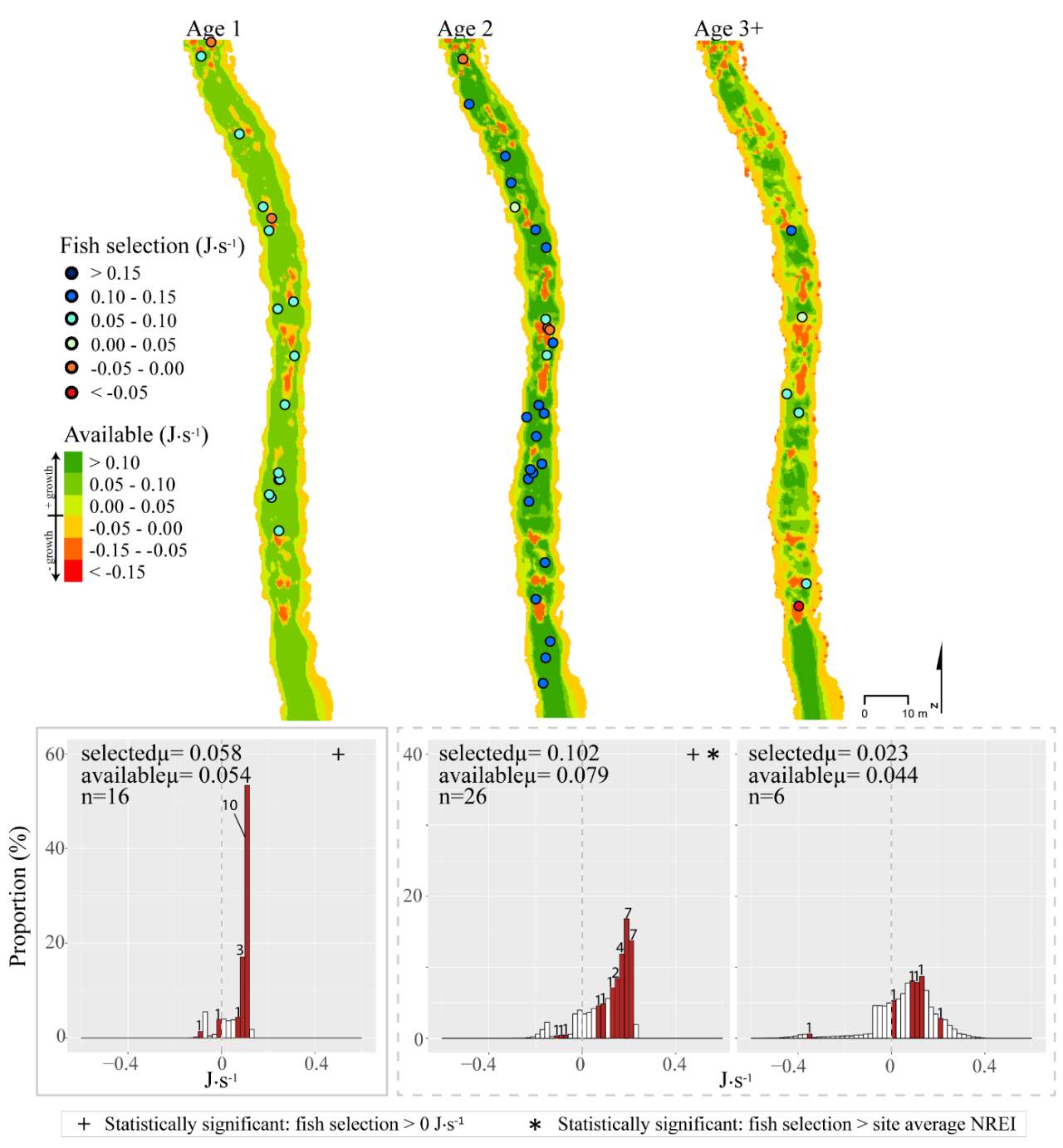
Figure 10. Forestry Camp, summer: used vs. available NREI distributions for each age class. The selected fish positions for each age class were mapped onto the depth-averaged NREI models of each site. a histogram was created which depicts the selected fish focal NREI estimate in red, and the available NREI distribution in white. In the histogram, the n value for each selected position is above the red bar.
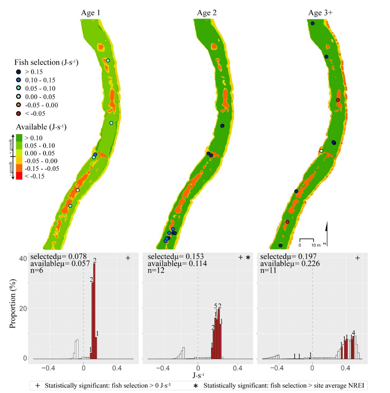
Figure 11. Forestry Camp, fall: used vs. available NREI distributions for each age class. The selected fish positions for each age class were mapped onto the depth-averaged NREI models of each site. a histogram was created which depicts the selected fish focal NREI estimate in red, and the available NREI distribution in white. In the histogram, the n value for each selected position is above the red bar.
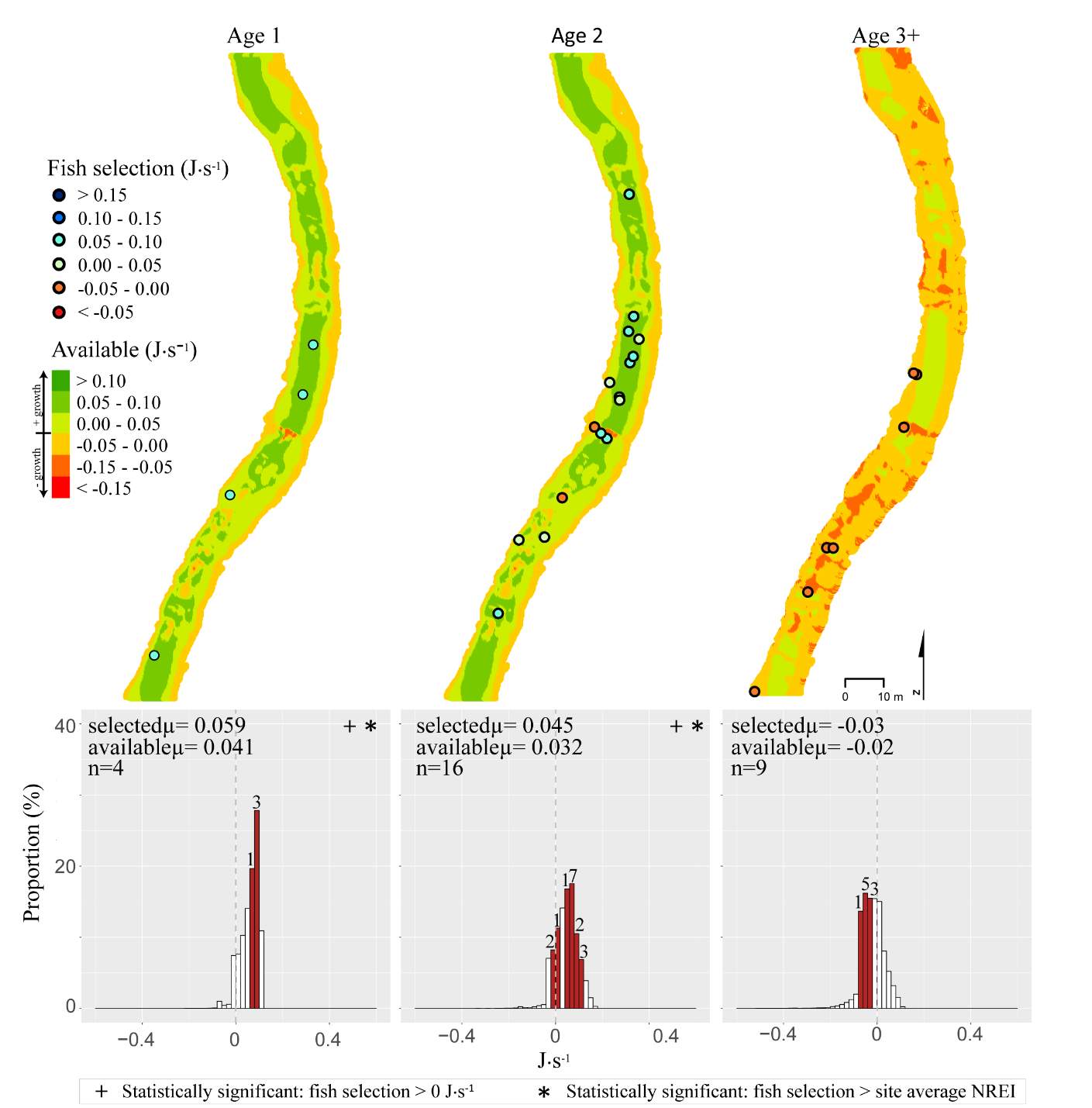
Figure 12. Spawn Creek, summer: used vs. available NREI distributions for each age class. The selected fish positions for each age class were mapped onto the depth-averaged NREI models of each site. a histogram was created which depicts the selected fish focal NREI estimate in red, and the available NREI distribution in white. In the histogram, the n value for each selected position is above the red bar.
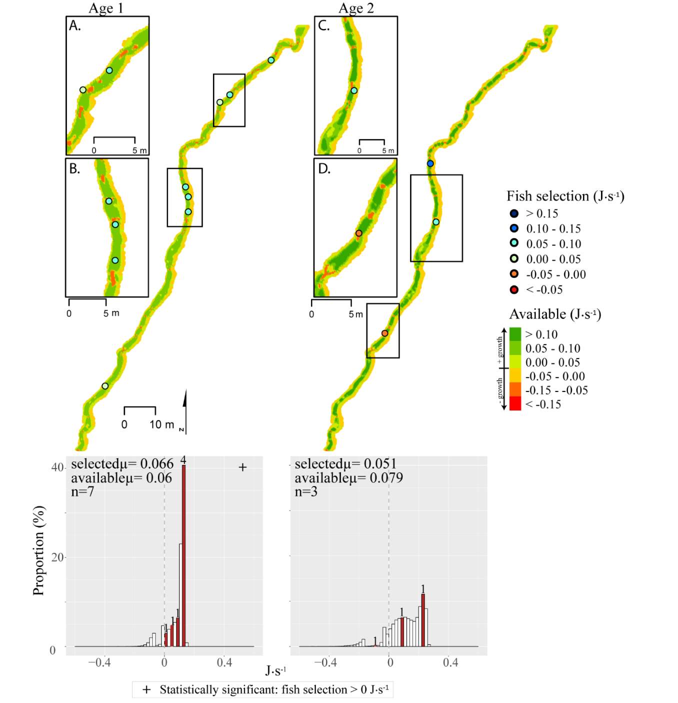
Figure 13. Spawn Creek, fall: used vs. available NREI distributions for each age class. The selected fish positions for each age class were mapped onto the depth-averaged NREI models of each site. a histogram was created which depicts the selected fish focal NREI estimate in red, and the available NREI distribution in white. In the histogram, the n value for each selected position is above the red bar.
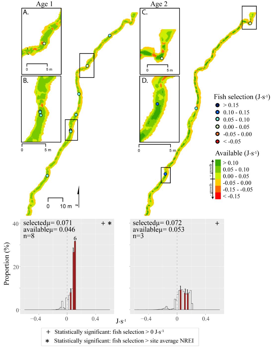
Figure 14. Beaver Creek, summer: used vs. available NREI distributions for each age class. The selected fish positions for each age class were mapped onto the depth-averaged NREI models of each site. a histogram was created which depicts the selected fish focal NREI estimate in red, and the available NREI distribution in white. In the histogram, the n value for each selected position is above the red bar.
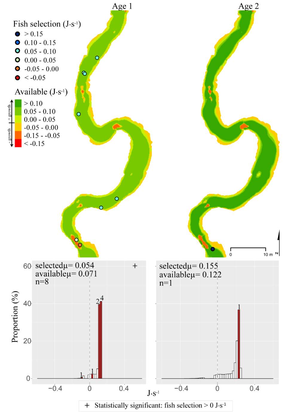
Figure 15. Franklin Basin, summer: used vs. available NREI distributions for each age class. The selected fish positions for each age class were mapped onto the depth-averaged NREI models of each site. a histogram was created which depicts the selected fish focal NREI estimate in red, and the available NREI distribution in white. In the histogram, the n value for each selected position is above the red bar.
2.3.3 Observed BCT densities vs. modeled carrying capacity
The maximum observed densities of BCT in the Logan River, between 2001-2015 (Budy, unpublished), were compared to NREI model predictions of carrying capacity for the most common size I encountered at each site (Beaver Creek – 125 mm; Forestry Camp – 150 mm; Franklin Basin – 100 mm; Red Banks – 150 mm; Spawn Creek – 125 mm). NREI-based carrying capacities were consistently higher than the abundances that have been observed over the last 15 years at each of the study sites (Figure 16). The linear regression between the observed and predicted carrying capacities were significant (R2=0.93, P=0.009; Figure 17). I also compared the predicted densities from each age class, rather than the most commonly observed fish size, to the maximum observed densities, while they were still related (R2=0.62, P=0.11), the relationship was not as strong (Figure 18). In addition, I tested two other metrics that have been used by past researchers: if the observed density of fish was related to the proportion of suitable habitat (R2=0.00, P = 0.98) and whether the fish biomass was related to the mean NREI at the site ( R2=0.08, P=0.67). There was no relationship between the observed fish density and the proportion of suitable habitat, and a weak relationship between the fish biomass and the mean NREI.
Figure 16. The most abundant years of BCT at each site, since 2001.
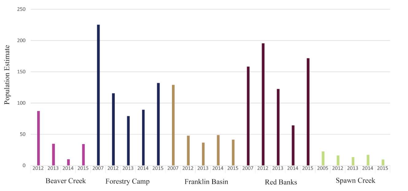
Figure 17. Linear regression of maximum observed BCT density’s relationship (by mode fish size) with NREI-based carrying capacity. A 1:1 line is provided for reference.
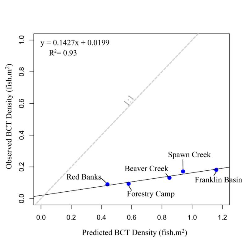
Figure 18. Linear regression of maximum observed BCT density’s relationship (by age class) with NREI-based carrying capacity. A 1:1 line is provided for reference.
2.4 Discussion
This study was designed to test whether the NREI model developed by Wall et al. (2015) could accurately characterize energetic habitat quality (i.e. fitness benefit) and carrying capacity for cutthroat trout. I compared the difference in the selected fish positions and the available NREI between August and October and between five hydraulically diverse sites in the Logan River watershed. I found that the majority (84%-100%) of over 200 observed fish were actively selecting for positions that the model predicted would allow them to gain body mass and that most (63%-100%) of Age 1 and Age 2 fish were selecting focal positions that were better than the site average, but less Age 3 fish were selecting better than the site average (33%-100%). Notably, only 3 fish were observed at one of my sites (Franklin Basin) and, only 1 of the 3 were selecting better than the site average (33%). Based on all other site data (sans Age 3 fish at Franklin Basin), the majority of Age 3 fish (67-100%) were selecting better than the site average. Age 1 and 2 fish were more selective than Age 3 fish overall, possibly due to less available habitat or less time spent foraging due to slowed growth rates recorded for Age 3 or older fish in the Logan River (Randall 2012). This research supports previous studies suggesting that NREI-type models can accurately identify habitats suitable for drift-feeding salmonids. In addition, I tested whether observed densities of BCT corresponded to the NREI model predicted carrying capacity and found that there was a strong relationship between these two variables. The results of this study are consistent with other bioenergetics model research that has shown that these models can be used to estimate NREI potential for salmonids, both at focal positions and as a measure of carrying capacity.
In this research, I found that the majority of younger fish (Age 1 and 2) used optimal focal positions in both seasons, when drift, temperature, and discharge all changed. Juvenile fish spatially distributed themselves in a non-random pattern, generally selecting the slow water directly adjacent to the faster water, near the center of each stream. This finding corroborates work done decades ago by Everest and Chapman (1972) and Fausch (1984), that showed fish should distribute themselves in this manner to maximize their NREI. While maintaining this position, fish can make short trips into the faster water collecting the drifting insects, while minimizing their swimming cost. The spatial distribution of these individual BCT supports ideas from optimal foraging theory (MacArthur and Pianka 1966), postulating that fish will forage the most efficiently possible to maximize their NREI, thus possessing greater fitness which allows for a better chance of reproductive success (Townsend and Winfield 1985).
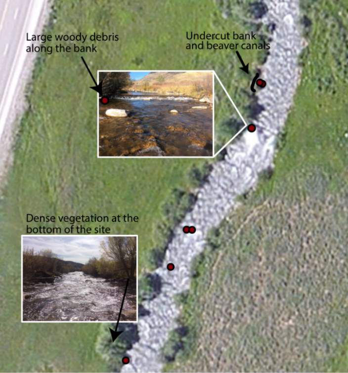
Although BCT generally occupied optimal positions, there were some exceptions where BCT were observed using positions that the model predicted as detrimental to growth (i.e. NREI -1). This result was most prevalent for Age 3 fish, especially in the fall, and much less characteristic of Age 1 and 2 fish. Randall (2012) found that individual BCT over 250 mm (i.e. Age 3+) were more sedentary in their movements and their growth rates had slowed in the Logan River. Similarly, Jenkins and Keeley (2010) found that there was significantly less habitat available at their study site for adult cutthroat trout, perhaps slowing their growth rates. In addition, Bachman (1984) found that older brown trout only occasionally foraged, in contrast to younger fish whom foraged very frequently. In this study, seasonal changes in stream temperature and drift abundance significantly altered the amount of habitat available for Age 3 fish. In fact, at Forestry Camp, the available NREI mean for Age 3 fish was -0.01 J·s-1, signifying that most spots were unsuitable for growth (Figure 11). Upon examination of the spatial dispersion of the adult fish, their spatial positioning suggests they were occupying focal positions near undercut banks and historic beaver canals, large woody debris, and near vegetative cover attached to the bank (Figure 19). These positions may provide a safe place to minimize their energy, while potentially, also providing cover from predators (Meehan et al. 1977).
Figure 19. Surveyed locations of Age 3+ cutthroat trout in October at the Forestry Camp site.
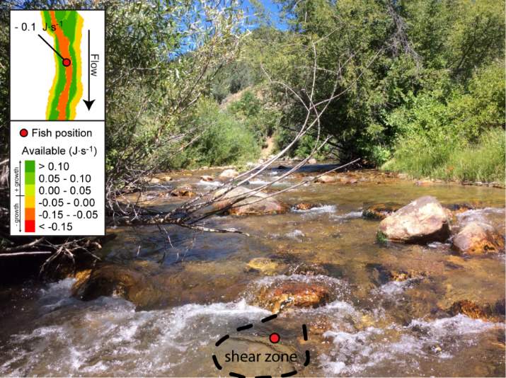
Overall, most of the observed fish were occupying focal positions that were better than available and would allow them to grow (Figure 8–Figure 15). However, some of the model predictions were not so accurate, predicting that the fish were using focal positions where they would lose weight (i.e. NREI -1). According to the field notes, all of the fish that the model predicted to lose weight were observed near cobble and boulder substrates. The NREI model is dependent upon the velocities in each fish location being accurately modeled, however, velocity predictions near or behind topographic complexities, such as instream boulders, could be higher in the hydraulic model than in the physical environment if the boulder was not surveyed. The stream bottom in the Logan River tends to be comprised of a bouldery, cobbly mixture, especially in the headwaters and at the mainstem sites. Large substrates force the flow around them, providing energy refugia (Wheaton et al. 2004) for foraging salmonids, and these large boulders usually have shear zones in the slow water behind them (on the downstream end). Figure 20 depicts a shear zone located behind a small boulder at the Franklin Basin site. In Figure 20, the fish is recorded as maintaining a focal position with an NREI below 0.0 J·s-1, meaning it would lose weight in this position. However, I hypothesize that the fish is maintaining a position in the lower velocity water, directly behind the boulder, but the local hydraulics are not captured because the boulder wasn’t surveyed. In the Logan, it was typical to observe fish in the energy refugia just downstream of boulders and cobbles, where they could wait for drift that was entrained in the thalweg. Since the Logan River is known for its rocky substrate, it is not feasible to survey every boulder and cobble. Therefore, some of these modeled errors are likely un-surveyed instream obstructions, where the hydraulic model is not capturing the actual stream topography. If the shear zone wasn’t modeled, these fish could negatively affect the significance of my results by reducing the selected NREI estimate for that site. To test whether shear zones could be affecting selected NREI values, I removed all of the fish that were associated with boulders at Franklin Basin and reran the Mann-Whitney test. Franklin Basin was chosen because it had some of the largest boulders and cobbles at all of my sites. It was also the toughest site to survey because of dense vegetation and a steep hillslope directly adjacent to the river which severely restricted my ability to survey these boulders and cobbles. At this site, NREI estimated focal positions for Age 2 and 3 fish were not significantly better than the available NREI at the site. However, when I removed the fish foraging near boulders and re-calculated the NREI selected estimate, the Age 2 fish were selecting focal foraging positions that were significantly better than the available NREI at the site (With boulders, Franklin Basin: Age 2; W=276.33, P=0.35: without boulders, W=887.77, P-1, Without boulders: mean NREI 0.13 J·s-1) indicating that fish foraging near boulders may have actually been maintaining positions in shear zones and negatively affecting the overall selected NREI value for that site. For a more detailed analysis of fish foraging near large instream obstructions, see Appendix A.
Figure 20. Depiction of a shear zone. Shear zones are found behind instream obstructions and provide energy refugia to salmonids. Shear zones are areas where fish can reduce swimming costs in the lower velocity water, but have access to the drifting insects in the higher velocity water, directly adjacent. Detecting shear zones in hydraulic model results requires that relevant flow obstructions are captured within survey topography.
The modeled carrying capacities were statistically associated with the observed densities in each study site, however the model predicted more fish than have been observed over the past 10 years at these sites. Although the Logan River supports one of the most abundant populations of BCT (Budy et al. 2007), it remains possible that these sites are underpopulated relative to their true theoretical carrying capacity. One such reason that these sites may not be at carrying capacity could be the presence of predators and competitors or other life history bottlenecks. Survival and growth of individual fish can be dependent upon shelter from predators and the proximity of this shelter to conserve energy. At each study site, brown trout, an introduced trout species, were either detected in this research or by other researchers also studying fish population dynamics in the Logan River (e.g., Budy et al. 2007, Randall 2012). While brown trout predation on cutthroat has not been confirmed (e.g., McHugh et al. 2008, Wood 2008), brown trout act as a competitor displacing BCT from energetically profitable positions (Wang and White 1994, McHugh et al. 2008), which can negatively affect growth and condition. When Budy et al. (2014) mechanically removed brown trout from a study site at Third Dam (a lower elevation Logan River mainstem site), the population of BCT increased by 20-fold, providing evidence that brown trout negatively affect cutthroat densities. Thus, the presence of brown trout at our sites may have decreased BCT abundance and accounts in part for the difference between observed fish and model predicted carrying capacity. In addition, overall, BCT densities are in decline in the Logan (Budy et al. 2007, Budy et al. 2014), suggesting that even though populations of BCT are abundant, they are likely not at carrying capacity.
Overall, the model successfully simulated BCT focal positions and predicted relative inter-site differences in carrying capacity, however there are model structure input changes that could improve model predictions, if not realism. For example, in the model, drift is set to the site average value for every available location; thus foraging success is not affected by drift captured by fish upstream, rather by the velocity speed, and the maximum capture distance of the fish. Since fish upstream are not modeled as reducing the prey available to fish downstream, simulations may over predict the carrying capacity of areas where drift has become depleted or locations where drift has settled out. Gowan and Fausch (2002) found that fish utilize stream positions based on the availability of drift, thus if drift was depleted or had settled out, fish would not be found foraging in that area. As such, previous research by Kotera and Inoue (2015) and Hayes et al. (2007), also found problems with uniform drift density assumptions and concluded that this simplification may cause model errors. Additionally, previous research has shown that maximum carrying capacity of a stream is based on a multitude of factors including (but not limited to) the maximum number of juvenile fish each year, the surface area available, and the territory size of each individual fish (Dumas and Prouzet 2003). For the sake of model simplicity, each of these parameters was not modeled in this research, rather a single fish size and territory size (based on the fish length) was used for each reach. A single territory size assumption may be problematic since at low population densities, individual fish will defend larger territories of optimal habitat, while at high population densities,individual fish will defend smaller territories of sub-optimal habitat (Ayllón et al. 2012). Nonetheless, although the model predicted much higher densities than have been observed over the past 10 year, the model was consistent in the over prediction of these densities. Therefore, if the intent of a research or management project was to gauge the relative habitat quality of multiple sites, based on how many fish the site could support, the NREI model could reliably be used in this function because the NREI models predictions had a strong relationship with the maximum abundance of fish at each site.
2.4.1 Management Implications
As part of the conservation agreement for BCT, three of the fourteen listed conservation strategies describe monitoring and improving BCT habitat quantity and quality (Lentsch et al. 2000). The NREI model used in this research has potential as a useful tool for managers to address these conservations strategies. Since the bioenergetics approach of modeling habitat selection is based on energetic costs and benefits, rather than correlations of physical habitat parameters, it allows for transferability between physically diverse streams. In this research, I used five sites that varied in depth, velocity, drift, and temperatures, and showed that the focal positions fish chose were reliably predicted by the model even in streams with very different physical characteristics. Further, impacts to streams, such as channel narrowing or water withdrawals, could alter depth, velocity, drift, or temperature, all of which are the main parameters of NREI models. Thus, NREI models could be used to simulate whether the project would result in degradation to trout habitats. For example, a common threat to stream habitats in the western US are water diversions for culinary or agricultural use (Moore et al. 1996), which have the potential to increase water temperatures (Meier et al. 2003). Before project implementation, managers could use NREI models to simulate temperature impacts to energetic habitat quality or quantity, which could provide quantitative analysis of habitat changes. Further, these models could be used to determine best-case restoration scenarios for BCT and other trout species. The model used in this research was previously tested on a steelhead restoration project in the Asotin watershed in Washington. Wall et al. (2016) modeled the effect large woody debris additions had on fish habitats. They were able to simulate the pre and post treatment changes to depth and velocity, revealing that the large woody debris additions increased the mean NREI available for steelhead salmon. Thus, modeling before and after changes to habitats offers a promising strategy for conserving and restoring BCT habitats and those of similar trout species.
2.4.2 Limitations
Although this study had many strengths, including surveying over 200 BCT focal positions in five physically diverse sites, it also had some limitations. The Logan River is a blue ribbon fishery with an abundant population of the BCT and other trout. The productivity of the Logan River could stem from ample drift densities and optimal temperatures for growth and spawning (0.01 J·s-1) ranged from a low of 61% suitable at the Red Banks site to a high of 96% suitable at Beaver Creek where drift densities were the largest sampled (6.14 g·m3). The proportion of suitable habitat made differences in behavior (i.e. foraging, holding, or moving) difficult to discern. Even when fish were recorded as holding on the bottom of the stream, the bioenergetics for that position was usually still favorable for growth. Thus, even though the NREI model is specific to drift-foraging, I was not able to discern differences in habitat use by behavior. Therefore, I recommend investigating differences in behaviors in streams that have a greater difference in drift densities and temperatures. Despite this recommendation, the model still effectively discriminated more favorable from less favorable habitats, relative to what the BCT used.
A second possible limitation to this study is that I used snorkeling as a method to identify the focal positions of individual BCT. Snorkeling has been criticized since some research has shown that the presence of snorkelers can alter salmonid behaviors (Brignon et al. 2011, Ellis et al. 2013). Despite criticisms, I found that while snorkeling in the Logan River, the coarse substrates (consisting of large of boulders and cobbles) and hydraulics allowed me to approach and observe fish in focal positions with minimal disturbance. Therefore, snorkeling as an observational method was not limiting in this river.
2.5 Conclusion
Previous researchers have suggested that bioenergetics models need to be tested for the species of interest before they are applied to management questions (Chipps and Wahl 2008). I found that the majority of observed fish were occupying focal positions that were better than available in 5 physically diverse stream reaches, with a wide variety of velocities, depths, drift and temperatures. The BCT chose positions in these reaches that would allow them to grow and survive (Figure 8-15), thus the bioenergetics model used in this research is useful for trout, especially for BCT. In addition, my research has corroborated research by Wall et al. (2015) that bioenergetics models can be used to identify reach-scale carrying capacity, allowing for innovative research on predictions of energetic habitat quality over large temporal and spatial scales with different environmental conditions. Thus, I believe bioenergetics models offers a promising alternative to traditional empirical correlations and physical habitat models, linking biotic and abiotic factors into a single measure of habitat quality.
Chapter 3
3.1 Conclusion
Assessments of habitat quality can be used to guide successful restoration strategies for endangered, threatened, and ‘conservation’ salmonid species or populations. Modeling approaches that accurately characterize habitat quality in mechanistic terms based on the factors that matter most to fish provide managers a means to rigorously assess potential impacts to streams and to more effectively manage restoration projects. Bioenergetics models offer a potential way to gauge energetic habitat quality beyond traditional correlative techniques, which suffer from transferability limitations and typically do not consider biotic factors (i.e. prey resources). Thus, my research has strengthened the technical basis for using bioenergetics models to quantify the fitness benefits of fluvial habitats, for BCT in particular and salmonids in general, and has the potential to inform habitat assessments or capacity estimation efforts focused at larger scales (e.g., Wheaton et al., In Revision).
3.1.1 Future Research Potential
To complement this research, there is potential to apply the NREI-derived measurements of energetic habitat quality by considering how they map to geomorphic features at different scales. Within sites (reaches), for instance, NREI distributions within particular geomorphic units (i.e. pool, riffle) can be examined to determine if there is a specific bioenergetics signature for different types of geomorphic units. Quantifying geomorphic unit–NREI associations is particularly useful because geomorphic units or particular assemblages or arrangements of units (e.g. a structurally-forced bar adjacent to a structurally-forced pool) can be mapped directly from topography (Wheaton et al. 2015) or assessed rapidly in the field (Camp and Wheaton 2014). Preliminary research at Spawn Creek (Figure 21) suggests that geomorphic units thought to provide fitness benefits to juvenile salmonids (i.e. concavities; pools) were predicted as the most energetically favorable by the NREI model (see Appendix B for more information). If geomorphic units have a bioenergetics signature, there is potential to rapidly assess streams and the geomorphic units therein in a stream for NREI potential. Identifiying bioenergetics signatures of geomorphic units would allow for management agencies to employ trained technicians to simply count geomorphic unit over long reaches, allowing for a complicated model to be used in a simpler, applied approach. Importantly, this line of inquiry may also facilitate the prediction of habitat value for entire riverscapes, assuming that geomorphic unit assemblages can be linked to other globally available network attributes (Wheaton et al., In Revision). Together, these lines of inquiry will eventually allow researchers and managers to harness the insights of complex, data-intensive models like NREI at unprecedented spatial scales.
Figure 21. Preliminary research on the mean energetic habitat quality within geomorphic units at Spawn Creek.
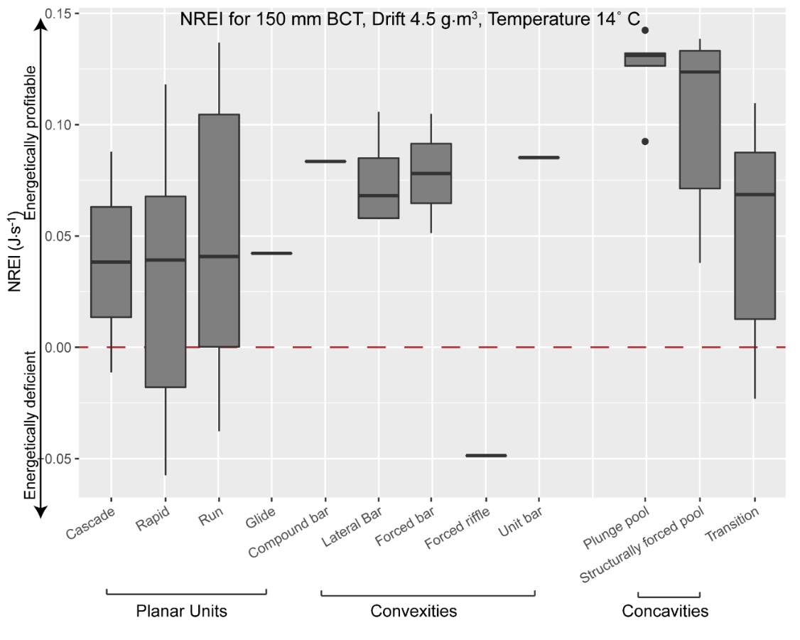
References
Addley, R. C. 1993. A mechanistic approach to modeling habitat needs of drift-feeding salmonids.
Al-Chokhachy, R. and P. Budy. 2007. Summer microhabitat use of fluvial bull trout in eastern Oregon streams. North American Journal of Fisheries Management 27:1068-1081.
Anlauf-Dunn, K. J., E. J. Ward, M. Strickland, K. Jones, and M. Bradford. 2014. Habitat connectivity, complexity, and quality: predicting adult coho salmon occupancy and abundance. Canadian Journal of Fisheries and Aquatic Sciences 71:1864-1876.
Ayllón, D., A. Almodóvar, G. G. Nicola, I. Parra, and B. Elvira. 2012. Modelling carrying capacity dynamics for the conservation and management of territorial salmonids. Fisheries Research 134:95-103.
Bachman, R. A. 1984. Foraging Behavior of Free-Ranging Wild and Hatchery Brown Trout in a Stream. Transactions of the American Fisheries Society 113:1-32.
Bangen, S., J. Wheaton, N. Bouwes, C. Jordan, C. Volk, and M. B. Ward. 2014. Crew variability in topographic surveys for monitoring wadeable streams: a case study from the Columbia River Basin. Earth Surface Processes and Landforms:n/a-n/a.
Behnke, R. 2010. Trout and salmon of North America. Simon and Schuster.
Bouwes, N., J. Moberg, N. Weber, B. Bouwes, C. Beasley, S. Bennett, A. Hill, C. Jordan, R. Miller, and P. Nelle. 2011. Scientific protocol for salmonid habitat surveys within the Columbia Habitat Monitoring Program. Prepared by the Integrated Status and Effectiveness Monitoring Program and published by Terraqua, Inc., Wauconda, Washington. Inc., Wauconda, WA.
Bovee, K. D. 1986. Development and evaluation of habitat suitability criteria for use in the instream flow incremental methodology. USDI Fish and Wildlife Service.
Brierley, G. J. and K. A. Fryirs. 2013. Geomorphology and river management: applications of the river styles framework. John Wiley & Sons.
Brignon, W. R., M. B. Davis, D. E. Olson, H. A. Schaller, and C. B. Schreck. 2011. Snorkelers’ in-water observations can alter salmonid behavior. Journal of Fish and Wildlife Management 2:90-98.
Budy, P., P. McHugh, G. P. Thiede, and E. VanDyke. 2003. Logan River whirling disease study: factors affecting trout population dynamics, abundance, and distribution in the Logan River, Utah. Annual Report to Utah Division of Wildlife Resources. Utah Cooperative Fish and Wildlife Research Unit, Logan, Utah.
Budy, P., G. P. Thiede, and P. McHugh. 2007. Quantification of the vital rates, abundance, and status of a critical, endemic population of Bonneville cutthroat trout. North American Journal of Fisheries Management 27:593-604.
Budy, P., G. P. Thiede, C. W. Saunders, C. S. Meredith, H. Mohn, J. Augspurger, and B. Roholt. 2014. Logan River trout viability: long-term monitoring and evaluation. US Geological Survey, Utah Cooperative Fish and Wildlife Research Unit Department of Watershed Sciences, Utah State University, Logan, Utah.
Camp, R. J. and J. M. Wheaton. 2014. Streamlining field data collection with mobile apps. Eos, Transactions American Geophysical Union 95:453-454.
CHaMP. 2015. Scientific protocol for salmonid habitat surveys within the Columbia Habitat Monitoring Program. Prepared by the Columbia Habitat Monitoring Program.
Chipps, S. R. and D. H. Wahl. 2008. Bioenergetics modeling in the 21st century: reviewing new insights and revisiting old constraints. Transactions of the American Fisheries Society 137:298-313.
Delft, d. 2016. Delft 3d. Deltares, The Netherlands.
Dumas, J. and P. Prouzet. 2003. Variability of demographic parameters and population dynamics of Atlantic salmon Salmo salar L. in a south-west French river. ICES Journal of Marine Science: Journal du Conseil 60:356-370.
Ellis, T. R., T. Linnansaari, and R. A. Cunjak. 2013. Passive integrated transponder (PIT) tracking versus snorkeling: quantification of fright bias and comparison of techniques in habitat use studies. Transactions of the American Fisheries Society 142:660-670.
ESRI. 2014. ArcGIS Desktop: Release 10.2.2. Environmental Systems Research Institute, Redlands, CA.
Everest, F. H. and D. W. Chapman. 1972. Habitat Selection and Spatial Interaction by Juvenile Chinook Salmon and Steelhead Trout in Two Idaho Streams. Journal of the Fisheries Research Board of Canada 29:91-100.
Fausch, K. D. 1984. Profitable stream positions for salmonids: relating specific growth rate to net energy gain. Canadian Journal of Zoology 62:441-451.
Fretwell, S. D. 1972. Populations in a seasonal environment. Princeton University Press.
Gowan, C. and K. D. Fausch. 2002. Why do foraging stream salmonids move during summer? Pages 139-153 Ecology, behaviour and conservation of the charrs, genus Salvelinus. Springer.
Gregory, S. V. and P. A. Bisson. 1997. Degradation and loss of anadromous salmonid habitat in the Pacific Northwest. Pages 277-314 Pacific Salmon & Their Ecosystems. Springer.
Guensch, G., T. Hardy, and R. Addley. 2001. Examining feeding strategies and position choice of drift-feeding salmonids using an individual-based, mechanistic foraging model. Canadian Journal of Fisheries and Aquatic Sciences 58:446-457.
Hafs, A. W., L. R. Harrison, R. M. Utz, and T. Dunne. 2014. Quantifying the role of woody debris in providing bioenergetically favorable habitat for juvenile salmon. Ecological Modelling 285:30-38.
Hauer, F. R. and G. A. Lamberti. 2011. Methods in stream ecology. Academic Press.
Hayes, J. W., N. F. Hughes, and L. H. Kelly. 2007. Process-based modelling of invertebrate drift transport, net energy intake and reach carrying capacity for drift-feeding salmonids. Ecological Modelling 207:171-188.
Hayes, J. W., J. D. Stark, and K. A. Shearer. 2000. Development and test of a whole-lifetime foraging and bioenergetics growth model for drift-feeding brown trout. Transactions of the American Fisheries Society 129:315-332.
Hepworth, D. K., M. J. Ottenbacher, and L. N. Berg. 1997. Distribution and abundance of native Bonneville cutthroat trout (Oncorhynchus clarki utah) in southwestern Utah. The Great Basin Naturalist:11-20.
Hilderbrand, R. H. and J. L. Kershner. 2000. Conserving inland cutthroat trout in small streams: how much stream is enough? North American Journal of Fisheries Management 20:513-520.
House, R. 1995. Temporal variation in abundance of an isolated population of cutthroat trout in western Oregon, 1981–1991. North American Journal of Fisheries Management 15:33-41.
Hughes, N. F. and L. M. Dill. 1990. Position Choice by Drift-Feeding Salmonids: Model and Test for Arctic Grayling (Thymallus arcticus) in Subarctic Mountain Streams, Interior Alaska. Canadian Journal of Fisheries and Aquatic Sciences 47:2039-2048.
Hughes, N. F., J. W. Hayes, K. A. Shearer, and R. G. Young. 2003. Testing a model of drift-feeding using three-dimensional videography of wild brown trout, Salmo trutta , in a New Zealand river. Canadian Journal of Fisheries & Aquatic Sciences 60:1462-1476.
Imre, I., J. Grant, and E. Keeley. 2004. The effect of food abundance on territory size and population density of juvenile steelhead trout (Oncorhynchus mykiss). Oecologia 138:371-378.
ISEMP/CHaMP. 2015. Combined Annual Report for the Integrated Status and Effectiveness Monitoring Program and Columbia Habitat Monitoring Pogram: 2014. Bonneville Power Administration.
iUtah. 2015. iUTAH: Science and Education for Utah’s Water Future.
iUTAH, C. T. 2016. Discharge Rating Curve at Logan River near Tony Grove Basic Aquatic Site (LR_TG_BA). iUTAH Modeling & Data Federation.
Jenkins, A. R. and E. R. Keeley. 2010. Bioenergetic assessment of habitat quality for stream-dwelling cutthroat trout (Oncorhynchus clarkii bouvieri) with implications for climate change and nutrient supplementation. Canadian Journal of Fisheries and Aquatic Sciences 67:371-385.
Jobling, M. 1995. Fish bioenergetics. Oceanographic Literature Review 9:785.
Katz, J., P. B. Moyle, R. M. Quiñones, J. Israel, and S. Purdy. 2013. Impending extinction of salmon, steelhead, and trout (Salmonidae) in California. Environmental Biology of Fishes 96:1169-1186.
Kotera, N. and M. Inoue. 2015. Position choice by red-spotted masu salmon: applicability of a bioenergetics model to habitat evaluation of headwater streams in southwestern Japan. Landscape and Ecological Engineering 11:119-128.
Lentsch, L. D., C. A. Toline, J. L. Kershner, J. M. Hudson, and J. Mizzi. 2000. Range-Wide Conservation Agreement and Strategy for Bonneville Cutthroat Trout (Oncorhynchus clarki utah).in U. D. o. W. Resources, editor., SLC, UT.
Lohn, D. R. 2008. Endangered Species Act Section 7 (a)(2) Consultation Biological Opinion and Magnuson-Stevens Fishery Conservation and Management Act Essential Fish Habitat Consultation.
MacArthur, R. H. and E. R. Pianka. 1966. On optimal use of a patchy environment. American Naturalist:603-609.
McHugh, P. and P. Budy. 2005. An experimental evaluation of competitive and thermal effects on brown trout (Salmo trutta) and Bonneville cutthroat trout (Oncorhynchus clarkii utah) performance along an altitudinal gradient. Canadian Journal of Fisheries and Aquatic Sciences 62:2784-2795.
McHugh, P., P. Budy, G. Thiede, and E. VanDyke. 2008. Trophic relationships of nonnative brown trout, Salmo trutta, and native Bonneville cutthroat trout, Oncorhynchus clarkii utah, in a northern Utah, USA river. Environmental Biology of Fishes 81:63-75.
Meehan, W. R., F. J. Swanson, and J. R. Sedell. 1977. Influences of riparian vegetation on aquatic ecosystems with particular reference to salmonid fishes and their food supply. USDA Forest Service General Technical Report RM (USA).
Meier, W., C. Bonjour, A. Wüest, and P. Reichert. 2003. Modeling the effect of water diversion on the temperature of mountain streams. Journal of Environmental Engineering 129:755-764.
Meredith, C. S., P. Budy, M. B. Hooten, and M. O. Prates. 2016. Assessing conditions influencing the longitudinal distribution of exotic brown trout (Salmo trutta) in a mountain stream: a spatially-explicit modeling approach. Biological Invasions:1-17.
Meredith, C. S., P. Budy, and G. P. Thiede. 2014. Predation on native sculpin by exotic brown trout exceeds that by native cutthroat trout within a mountain watershed (Logan, UT, USA). Ecology of Freshwater Fish 24:133-147.
Mohn, H. 2016. Aligning Conservation Goals and Management Objectives for Bonneville Cutthroat Trout (Oncorhynchus Clarki Utah) in the Logan River, Utah.
Moore, M. R., A. Mulville, and M. Weinberg. 1996. Water allocation in the American West: Endangered fish versus irrigated agriculture. Nat. Resources J. 36:319.
Naiman, R. J., J. R. Alldredge, D. A. Beauchamp, P. A. Bisson, J. Congleton, C. J. Henny, N. Huntly, R. Lamberson, C. Levings, and E. N. Merrill. 2012. Developing a broader scientific foundation for river restoration: Columbia River food webs. Proceedings of the National Academy of Sciences 109:21201-21207.
Nickelson, T. E., J. D. Rodgers, S. L. Johnson, and M. F. Solazzi. 1992. Seasonal changes in habitat use by juvenile Coho salmon (Oncorhynchus kisutch) in Oregon coastal streams. Canadian Journal of Fisheries and Aquatic Sciences 49:783-789.
NOAA. 2012. Upper Columbia Spring Chinook & Steelhead Recovery Plan:: NOAA Fisheries.
O’Neal, J. S. 2007. Snorkel surveys. American Fisheries Society. Salmonid Field Protocols Handbook. Bethesda, Maryland:325-340.
Peck, D. V., J. M. Lazorchak, and D. J. Klemm. 2001. Environmental Monitoring and Assessment Program–surface Waters: Western Pilot Study Field Operations Manual for Wadeable Streams. National Health and Environmental Effects Research Laboratory [and] National Exposure Research Laboratory, Office of Research and Development, US Environmental Protection Agency.
Platts, W. S. and R. L. Nelson. 1988. Fluctuations in trout populations and their implications for land-use evaluation. North American Journal of Fisheries Management 8:333-345.
Raleigh, R. F., W. J. Miller, and P. C. Nelson. 1986. Habitat Suitability Index Models and Instream Flow Suitability Curves: Chinook Salmon. DTIC Document.
Randall, J. W. 2012. The survival and growth of adult Bonneville Cutthroat Trout (Oncorhynchus clarkii utah) in response to different movement patterns in a tributary of the Logan River, Utah.
Roni, P. and T. P. Quinn. 2001. Density and size of juvenile salmonids in response to placement of large woody debris in western Oregon and Washington streams. Canadian Journal of Fisheries and Aquatic Sciences 58:282-292.
Roper, B. B., D. L. Scarnecchia, and T. J. La Marr. 1994. Summer Distribution of and Habitat Use by Chinook Salmon and Steelhead within a Major Basin of the South Umpqua River, Oregon. Transactions of the American Fisheries Society 123:298-308.
Rosenfeld, J. 2003. Assessing the Habitat Requirements of Stream Fishes: An Overview and Evaluation of Different Approaches. Transactions of the American Fisheries Society 132:953-968.
Rosenfeld, J., H. Beecher, and R. Ptolemy. 2016. Developing Bioenergetic-Based Habitat Suitability Curves for Instream Flow Models. North American Journal of Fisheries Management 36:1205-1219.
Rosenfeld, J. S. and S. Boss. 2001. Fitness consequences of habitat use for juvenile cutthroat trout: energetic costs and benefits in pools and riffles. Canadian Journal of Fisheries & Aquatic Sciences 58:585-593.
Rosenfeld, J. S., T. Leiter, G. Lindner, and L. Rothman. 2005. Food abundance and fish density alters habitat selection, growth, and habitat suitability curves for juvenile coho salmon (Oncorhynchus kisutch). Canadian Journal of Fisheries & Aquatic Sciences 62:1691-1701.
Rosenfeld, J. S. and W. Tonn. 2014. Modelling the effects of habitat on self-thinning, energy equivalence, and optimal habitat structure for juvenile trout. Canadian Journal of Fisheries & Aquatic Sciences 71:1395-1406.
Smith, E. A., R. L. Bettinger, C. A. Bishop, V. Blundell, E. Cashdan, M. J. Casimir, A. L. Christenson, B. Cox, R. Dyson-Hudson, and B. Hayden. 1983. Anthropological Applications of Optimal Foraging Theory: A Critical Review [and Comments and Reply]. Current Anthropology:625-651.
Smith, T. A. and C. E. Kraft. 2005. Stream fish assemblages in relation to landscape position and local habitat variables. Transactions of the American Fisheries Society 134:430-440.
Smock, L. A. 1980. Relationships between body size and biomass of aquatic insects. Freshwater Biology 10:375-383.
Smokorowski, K. E. and T. C. Pratt. 2007. Effect of a change in physical structure and cover on fish and fish habitat in freshwater ecosystems – a review and meta-analysis. Environmental Reviews 15:15-41.
Team, R. C. C. 2016. R: A language and environment for statistical computing. R Foundation for Statistical Computing. Vienna, Austria.
Teuscher, D. and J. Capurso. 2007. Management plan for conservation of Bonneville Cutthroat Trout in Idaho. Idaho Department of Fish and Game. Boise, Idaho.
Townsend, C. R. and I. J. Winfield. 1985. The application of optimal foraging theory to feeding behaviour in fish. Pages 67-98 Fish energetics. Springer.
Urabe, H., M. Nakajima, M. Torao, and T. Aoyama. 2010. Evaluation of habitat quality for stream salmonids based on a bioenergetics model. Transactions of the American Fisheries Society 139:1665-1676.
USDOI, B. 2001. Wyoming. 2001. Sensitive species policy and list. Bureau of Land Management, Wyoming State Office, Cheyenne, Wyoming. Instruction memorandum no. WY-2001-040.
USGS. 2001. National Water Information System data available on the World Wide Web (Water Data for the Nation).
Wall, C. E. 2014. Use of a net rate of energy intake model to examine differences in juvenile steelhead (Oncorhynchus mykiss) densities and the energetic implications of restoration.
Wall, C. E., N. Bouwes, J. M. Wheaton, S. Bennett, W. C. Sauders, P. McHugh, and C. Jordan. 2016. Design and monitoring of woody structures and their benefits to juvenile steelhead trout (Oncorhynchus mykiss) using a net rate of energy intake model. Canadian Journal of Fisheries & Aquatic Sciences.
Wall, C. E., N. Bouwes, J. M. Wheaton, W. C. Saunders, and S. N. Bennett. 2015. Net rate of energy intake predicts reach-level steelhead (Oncorhynchus mykiss) densities in diverse basins from a large monitoring program. Canadian Journal of Fisheries and Aquatic Sciences:1-11.
Wang, L. and R. J. White. 1994. Competition between wild brown trout and hatchery greenback cutthroat trout of largely wild parentage. North American Journal of Fisheries Management 14:475-487.
Wankowski, J. 1979. Morphological limitations, prey size selectivity, and growth response of juvenile Atlantic salmon, Salmo salar. Journal of Fish Biology 14:89-100.
Weaver, D. M., T. J. Kwak, and K. H. Pollock. 2014. Sampling characteristics and calibration of snorkel counts to estimate stream fish populations. North American Journal of Fisheries Management 34:1159-1166.
Wheaton, J. M., K. A. Fryirs, G. Brierley, S. G. Bangen, N. Bouwes, and G. O’Brien. 2015. Geomorphic mapping and taxonomy of fluvial landforms. Geomorphology 248:273-295.
Wheaton, J. M., G. B. Pasternack, and J. E. Merz. 2004. Spawning habitat rehabilitation ‐ II. Using hypothesis development and testing in design, Mokelumne river, California, U.S.A. International Journal of River Basin Management 2:21-37.
Wood, J. R. 2008. An Investigation of the Early Life-history of Brown Trout (Salmo Trutta) and Potential Influences on Invasion Success in the Logan River, Utah. ProQuest.
Wurtsbaugh, W. A., N. A. Heredia, B. G. Laub, C. S. Meredith, H. E. Mohn, S. E. Null, D. A. Pluth, B. B. Roper, W. C. Saunders, and D. K. Stevens. 2014. Approaches for studying fish production: Do river and lake researchers have different perspectives? Canadian Journal of Fisheries and Aquatic Sciences 72:149-160.
Appendices
Appendix A: In-stream topographic complexities and their effect on the derived NREI value for BCT
This appendix provides supplementary material on the effect instream topographic complexities may have on the derived NREI value for each fish location. As described in Chapter 2, BCT occasionally selected spatial positions that the NREI model predicted would be conducive to losing weight. If large topographic complexities (i.e. substrates) were not surveyed, the hydraulic model results would not be accurate in these locations, and ultimately, the derived NREI value for each of these fish would be skewed. NREI results would be skewed because large boulders often have pockets of slow water just behind them, which would minimize swimming costs. However, if the large boulder was not surveyed, the pocket of slow water may not have been modeled in the hydraulic model, thus increasing swimming costs in this area. During my snorkel surveys, fish were often seen in these pockets of slow water (i.e. shear zones) behind the large boulders. However, since the CHaMP surveying methodology, used in this research, is designed to capture the stream bedform and avoid capturing substrate roughness elements (CHaMP, 2015), most of these topographic complexities were not surveyed to account for changes in velocities around them. The hydraulic modeling does include a stream roughness parameter which is based on the pebble counts at each site and represented as the D84 (ISEMP/CHaMP 2015). However, substrate roughness is modeled over the entire hydraulic model, and doesn’t necessarily capture the largest topographic complexities. Therefore if a boulder is larger than the D84, the shear zone around the boulder would only be as large as the D84, where in reality it is much larger (because the boulder was larger than the site’s D84 measurement). Shear zones, location behnd boulders larger than the site D84, would be represented as a much faster velocity within the hydraulic model. Thus, some fish may be foraging in shear zones behind boulders that are being projected as high velocity areas, but because the boulder wasn’t surveyed, the position the fish chose has a much higher velocity in the model than it does the physical environment.
The largest topographic complexities (i.e. boulders) are investigated in this appendix. Two of my sites, Beaver Creek and Spawn Creek, were not analyzed since there was only one fish observed near boulders between the two sites. To investigate large topographic complexities and their effect on the derived NREI value of each these fish, I used information that I collected during snorkel surveys, namely the substrate within 1 meter of each individual surveyed fish. The results of fish, by age group, and substrate selection is graphed in Figure A1. This graph indicates that certain age groups of fish were not more selective of certain substrates. Therefore, NREI results should not be skewed for one age class over another based on substrate selection. Of all my sites, Red Banks and Franklin Basin had mostly rough substrates which created a geomorphology characterized by rapids that contain large boulders and cobbles, forcing a variety of hydraulics surrounding these rough substrates, thus I observed a large number of shear zones at both of these sites. Conversely, the river through Forestry Camp is wider and the water is slower, than both Red Banks and Franklin Basin. Therefore I observed less shear zones at Forestry Camp than at Red Banks or Franklin Basin.
Figure A1. The recorded substrates within 1 meter of each fish, during snorkel surveys.
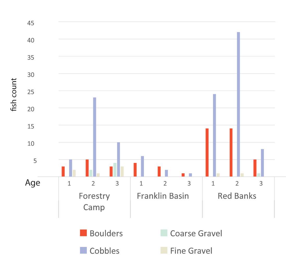
To test whether the boulders were causing the derived NREI values to be lower for fish near boulders, at each site, I removed fish that were foraging near boulders. Once I had removed fish foraging near boulders, I checked if the selected NREI differed between the average of all fish and the average if fish observed near boulders were removed (Figure A2). Overall, the mean NREI increased for each age class if fish foraging near boulders were removed from the analysis (Figure A3).
Figure A2. The mean NREI if all fish selected positions are averaged (by age class) and if fish found near boulders (potentially foraging in shear zones) are removed from the analysis at each site. The graph is divdied by season, site, and by age group of BCT.
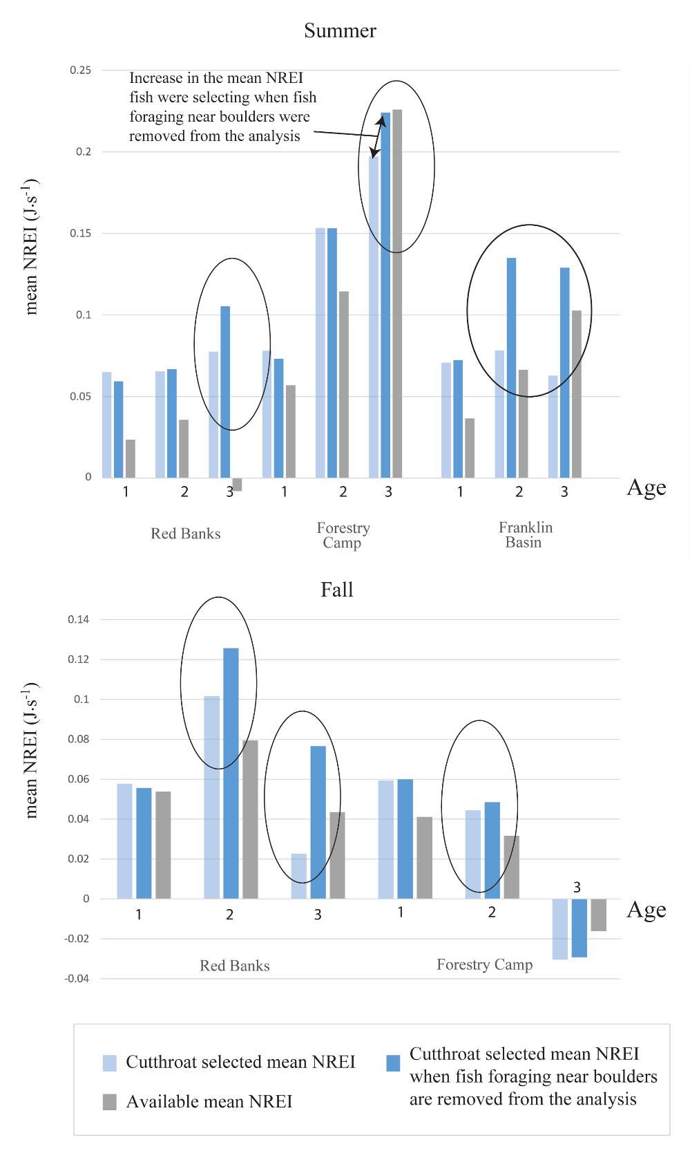
Figure A3. The relationship between the mean NREI selected and the mean NREI available at each site. A) The relationship with all surveyed fish and B) the relationship if fish foraging near boulders are removed from the analysis. A line with a slope of 1 is shown for reference.

Last of all, I re-tested the significance of whether fish had selected better habitat than available (i.e. Selected NREI > Available NREI) if fish observed near boulders were removed from the analysis. To test the significance, I used the non-parametric one-sided Mann Whitney U-test, since the available NREI distributions were not normally distributed. The test was used to determine if the median of selected NREI distributions was greater than the median of available NREI distributions. The available NREI points at each site far surpass the selected points at each site (n~250,000 available points at each site, n=9-62 selected points). To mitigate for the unbalanced distributions, 200 randomly sampled points were selected from the available NREI distributions. A Mann-Whitney test statistic was computed 10,000 times on the selected and randomly sampled available distributions, and averaged. Table A1 shows the results of the significance test.
Table A1. The results of the Mann-Whitney test if fish observed near boulders are removed from the analysis. An * indicates the results went from non-signficant to significant (i.e. the fish foraging near boulders had a significant negative effect on whether the selected NREI > available NREI), a (-) indicates the results went from significant to non-significant, a blank indicates no change.
| Age class | Beaver Creek | Forestry Camp | Franklin Basin | Red Banks | Spawn Creek | |
|
summer |
1 | |||||
| 2 | * | |||||
| 3 | na | |||||
|
fall |
1 | na | – | na | ||
| 2 | na | na | ||||
| 3 | na | na |
Overall, one age class of fish didn’t appear to select boulders over other substrates (Figure A2). However, although Age 2 and 3 fish weren’t more selective of boulders than other substrates, the older fish (age 2 and 3) that were observed near boulders were more likely to change the mean NREI selected and, in one case, the significance of selected NREI value for the fish location (Figure A3, Table A1). When fish observed near boulders were removed, the mean NREI value increased (Figure A3) at most sites and for most age classes. This mean NREI increase suggests that some fish may have been using shear zones behind boulders that were not accurately depicted by the hydraulic model. Subsequently, statistical testing didn’t show any major changes in the results presented in Chapter 2. Thus, as discussed in Chapter 2, most fish were selecting focal positions that the NREI model predicted as viable for gaining weight. However, since the mean NREI increased for most selected fish positions when fish found near large boulders were removed, the results of the preliminary research suggest that some large boulders (especially at Franklin Basin) may not have been surveyed enough to model the hydraulic refugia. For future research, I recommend surveying all of the shear zones and associated boulders that fish are found near. Once the shear zones are surveyed, rerun the hydraulic model and the NREI model and restest if fish foraging near boulders have a higher overall NREI if the boulders are surveyed.
Appendix B: Distribution of NREI values within geomorphic units at each site
This appendix provides supplementary material on whether geomorphic units or particular assemblages of geomorphic units exhibit charactieristic energetic signatures across different sites, temperatures, and drift values. For each site, I delineated the geomorphic units using the Geomorphic Unit Tool (GUT) and created a boxplot of the distribution of NREI values within each geomorphic unit. Data presented in this appendix is presented as 1) site map with delineated geomorphic units and 2) boxplots of distribution of NREI values within each geomorphic unit.
For each site, the the geomorphic units-NREI association were examined based on a single age class and a single vertical position within the water column. I examined geomorphic units for Age 2 BCT at the site-specific drift and temperature values. Age 2 fish were chosen because the fork length of 150 mm it is often used to create habitat suitability curves for juvenile steelhead (Holmes et al. 2014) and is, also a typical size of juvenile BCT found in the Logan River. To calculate NREI for each geomorphic unit, I assumed that juvenile salmonids often occupy foraging positions that are near the substrate (Jenkins and Keeley 2010), holding a position approximately 10 cm above the stream bottom where they can see prey drifting in the water column.
In order to calculate the geomorphic unit-NREI association, two models were run for each site: the GUT and the NREI. The GUT was used to delineate in-channel geomorphic units, while the NREI was used to determine the energetic quality of each geomorphic unit. For a description of the NREI, see section 2.2.3
Description of the Geomorphic Unit Tool
Topographic data from each of my CHaMP surveys were classified into individual geomorphic units using the Wheaton et al (2015) fluvial taxonomy framework. The fluvial taxonomy represents a hierarchical, systematic framework that allows for repeatable results across riverscapes (Wheaton et al. 2015). This framework is a based on topographic lines of evidence that leads to a distinct geomorphic unit delineation. Using a repeatable classification scheme removes the inherent error of analyzing patterns and classifying the same elements into different categories (Li and Wu 2004). This method was employed semi-automatically by using the Geomorphic Unit Tool (GUT), which derives vector polygons from the DEMs created for each reach. The output is three-tiered. The first tier contains information on whether the unit is an in-channel or out-of-channel unit, of which I will only be analyzing in-channel units. The second tier predicts whether the unit is a concavity, convexity, or planar unit. The third tier assigns whether the unit is bank attached, mid channel, or channel spanning and a probability score on the type of unit it is (i.e. an 80% probability the unit is a run). The GUT output for each site is shown in Figure B1–Figure B5.
Once the GUT was run for each site, the distribution of NREI values within each geomorphic unit were calculated. The NREI values were spatially joined to the closest geomorphic unit and then boxplots of distributions were calculated in R software (R Core Team 2016). The distribution of NREI values within each geomorphic unit, at each site, is shown in Figure B6–Figure B10.
Figure B1. The results of GUT at Spawn Creek, using a 55% capture rate and the drift and temperature at the time of snorkeling.
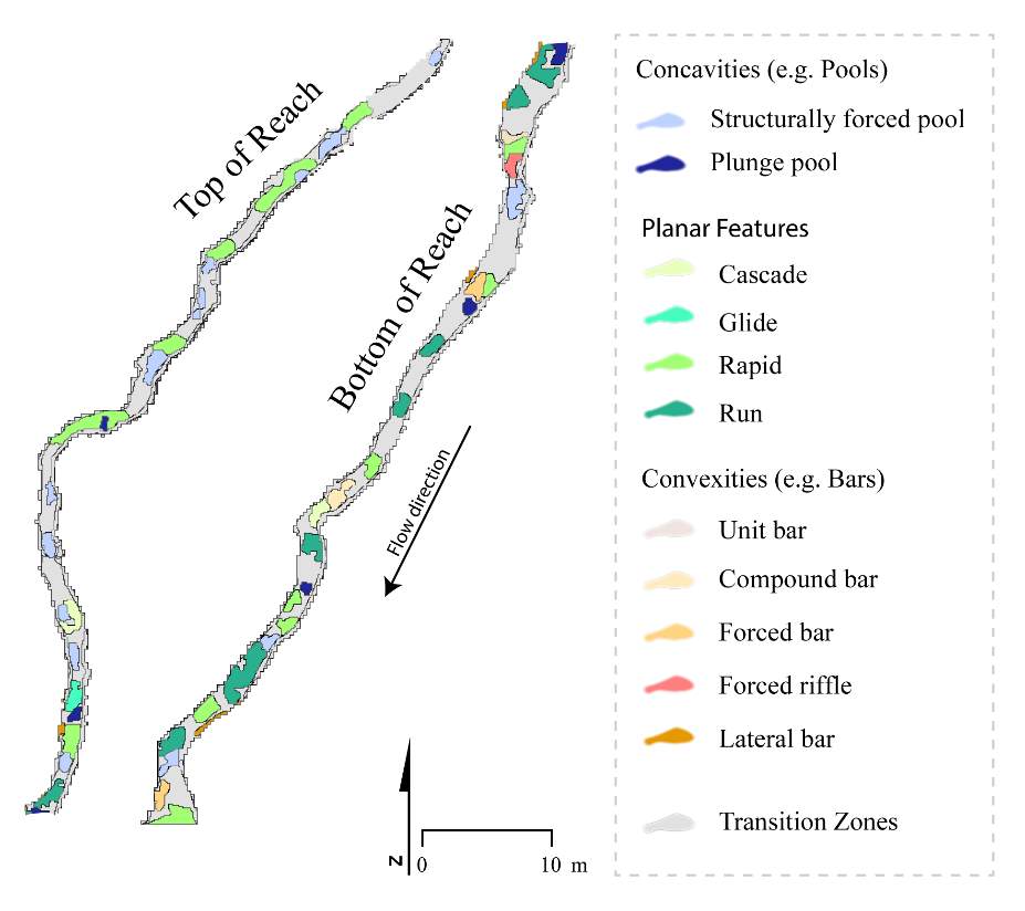
Figure B2. The results of GUT at Red Banks, using a 55% capture rate and the drift and temperature at the time of snorkeling.
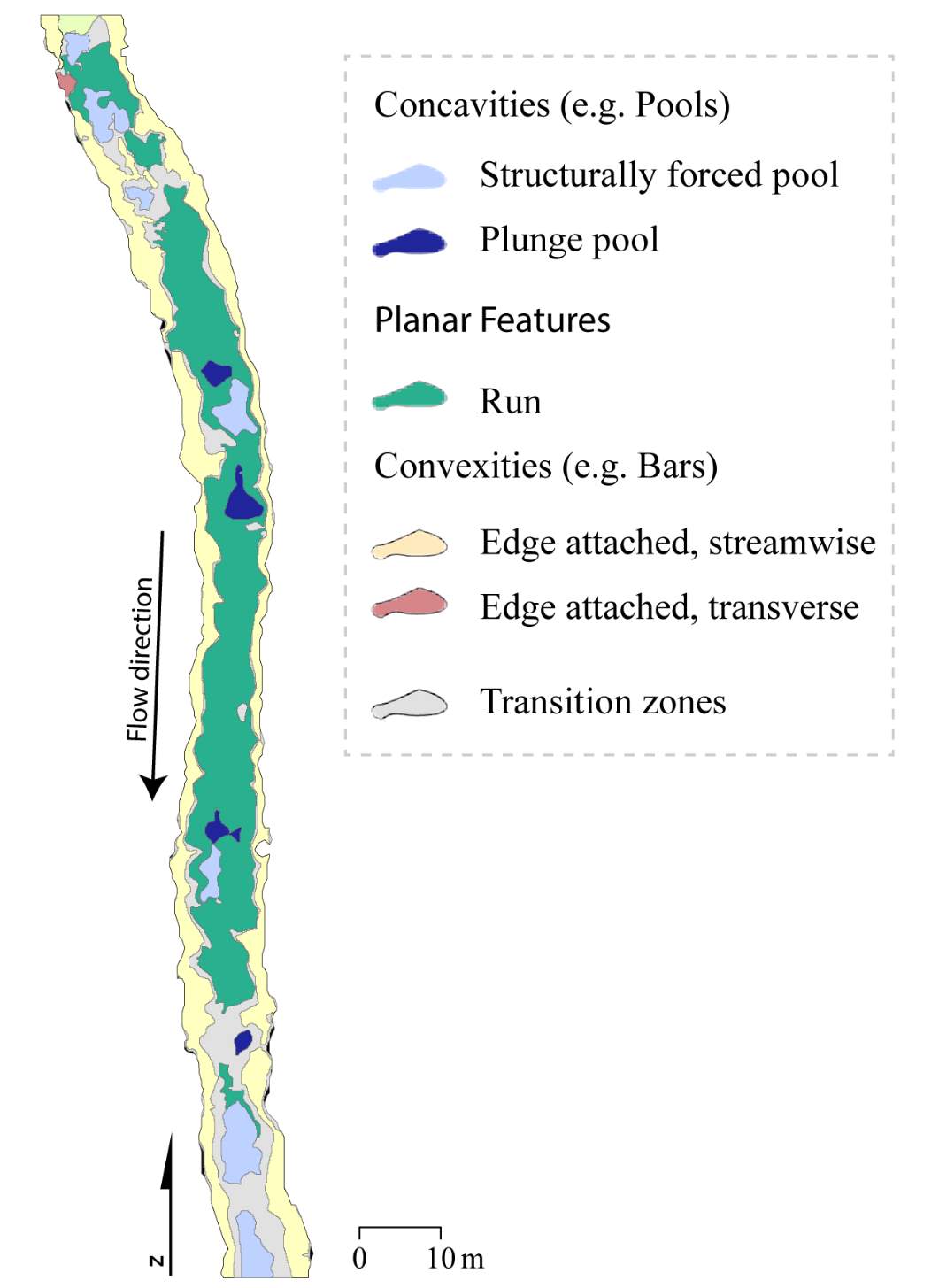
Figure B3. The results of GUT at Forestry Camp, using a 55% capture rate and the drift and temperature at the time of snorkeling.
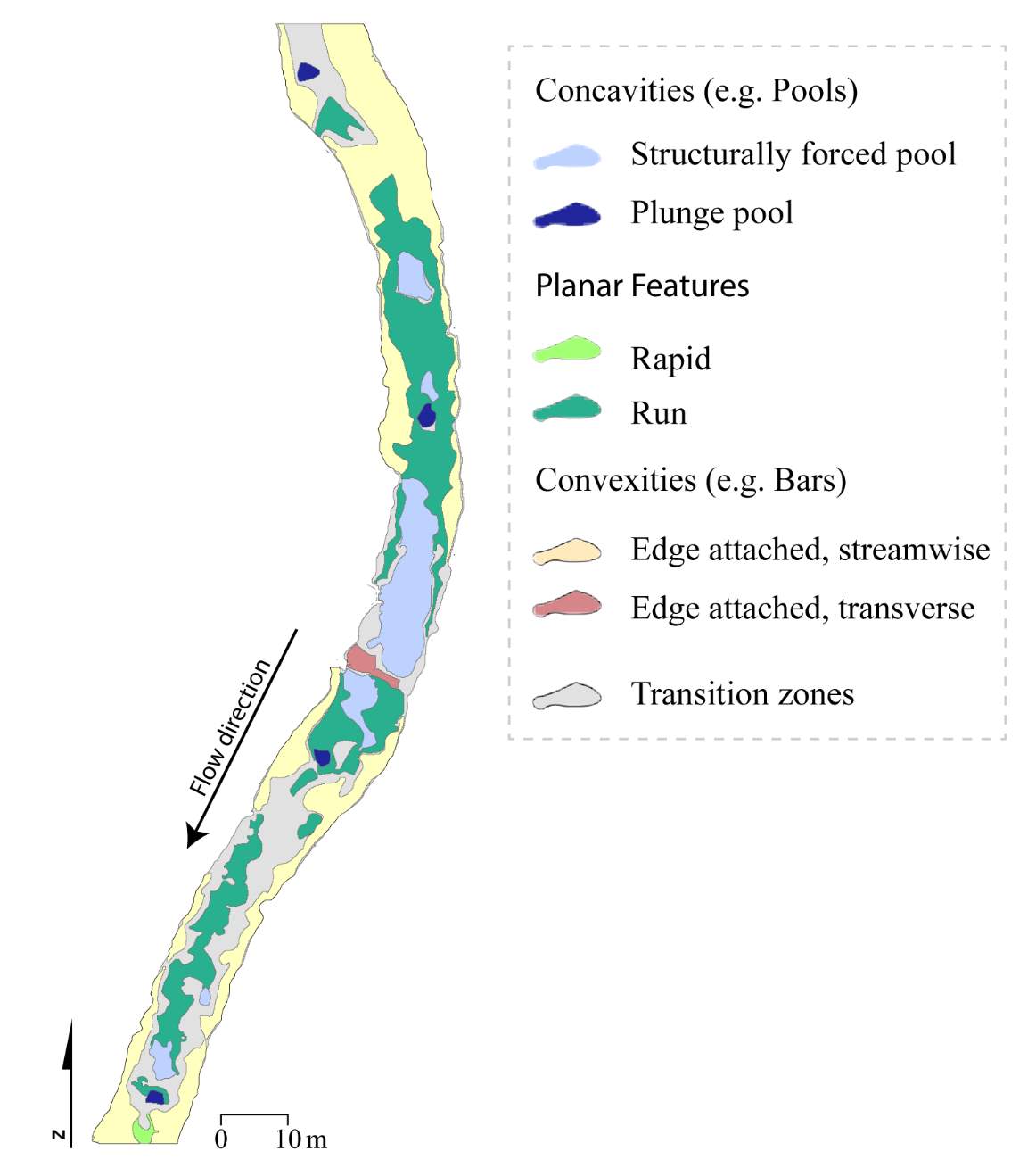
Figure B4. The results of GUT at Franklin Basin, using a 55% capture rate and the drift and temperature at the time of snorkeling.
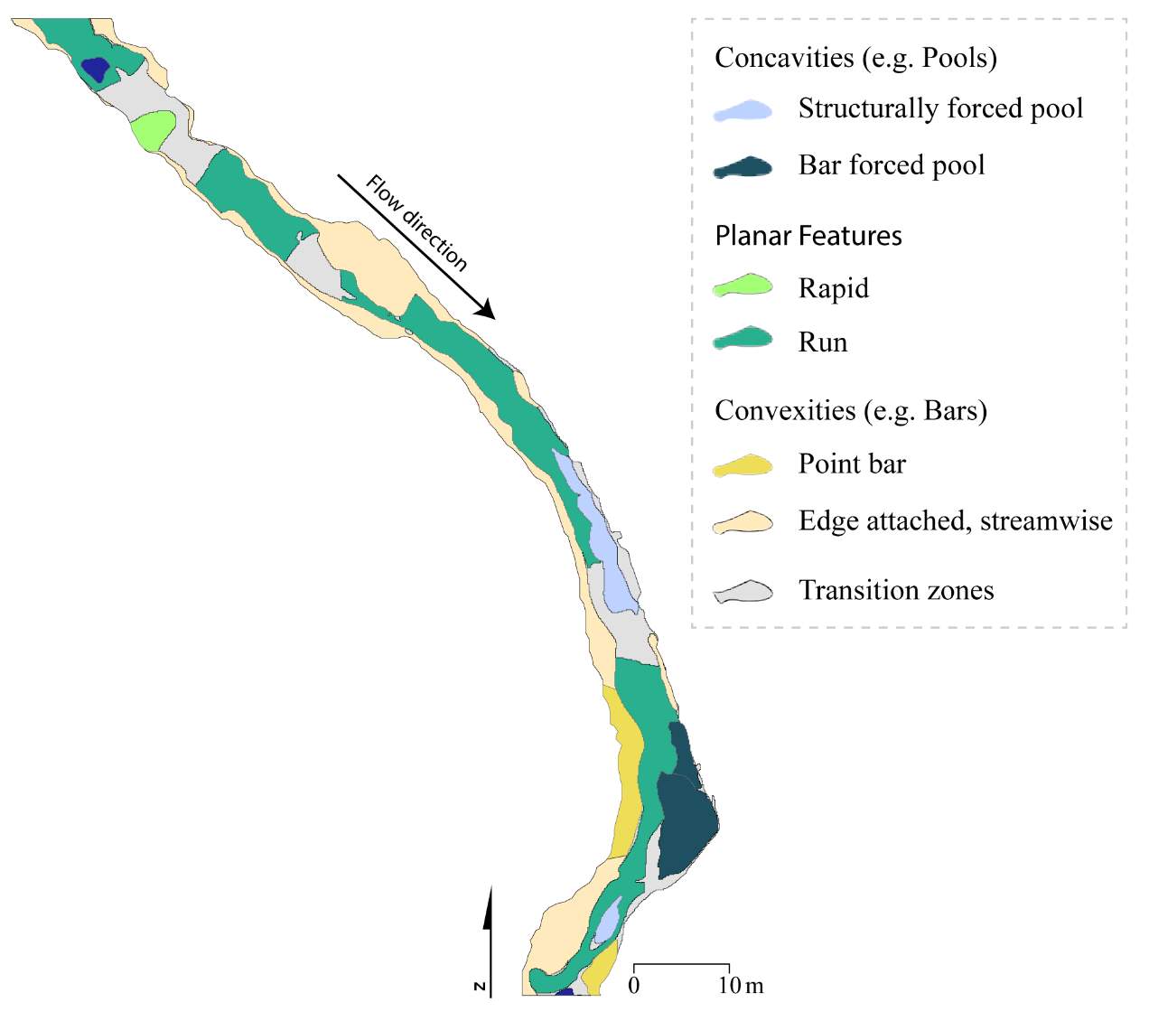
Figure B5. The results of GUT at Beaver Creek, using a 55% capture rate and the drift and temperature at the time of snorkeling.
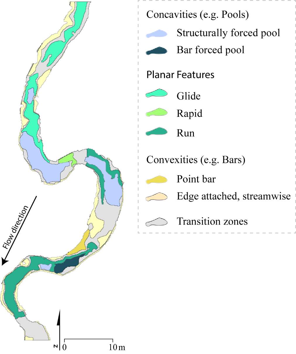
Figure B6. The distribution of NREI values within each geomorphic unit at Spawn Creek. The drift and temperature used were those collected during the snorkeling events: Drift 3.38 g.m3, temp 11.5° C.
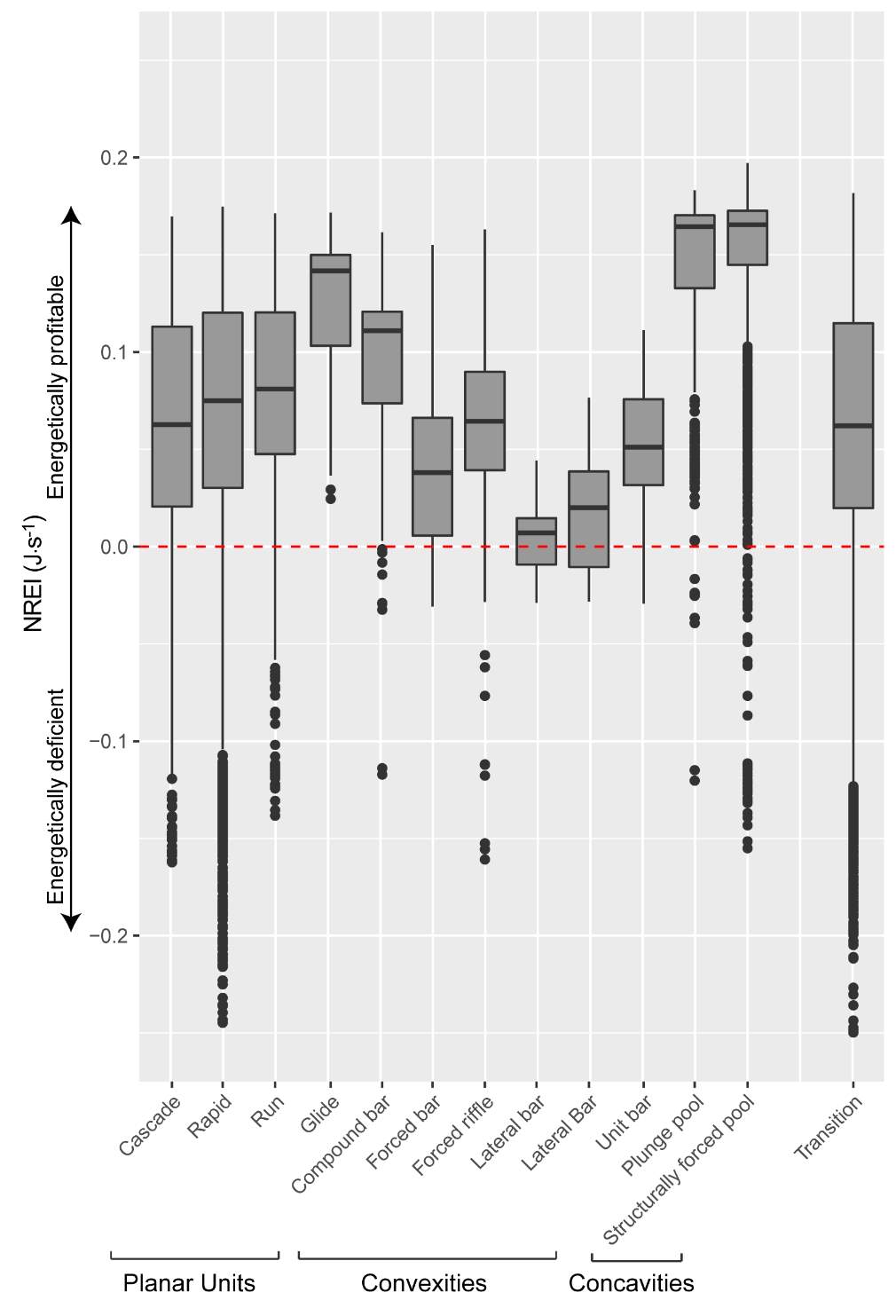
Figure B7. The distribution of NREI values within each geomorphic unit at Red Banks. The drift and temperature used were those collected during the snorkeling events: Drift 1.65 g.m3, temp 11.4° C.
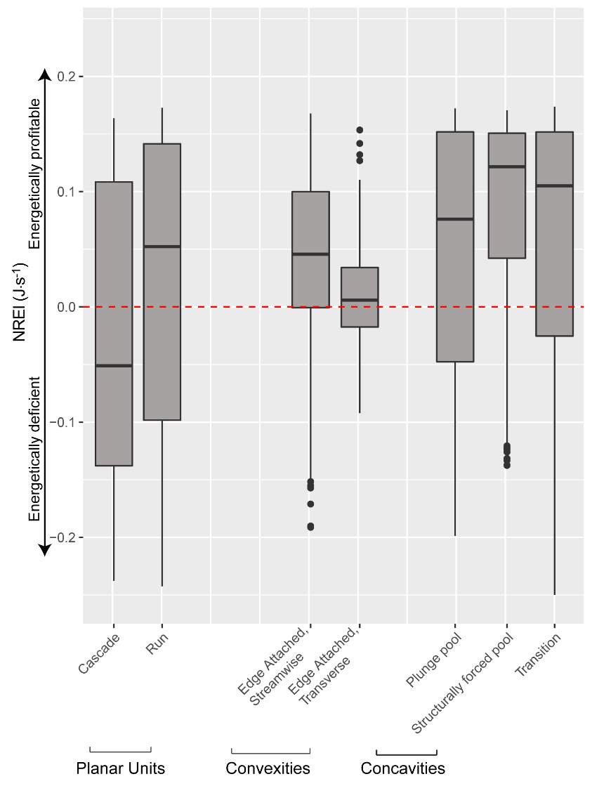
Figure B8. The distribution of NREI values within each geomorphic unit at Forestry Camp. The drift and temperature used were those collected during the snorkeling events: Drift 1.77 g.m3, temp 11.7° C.
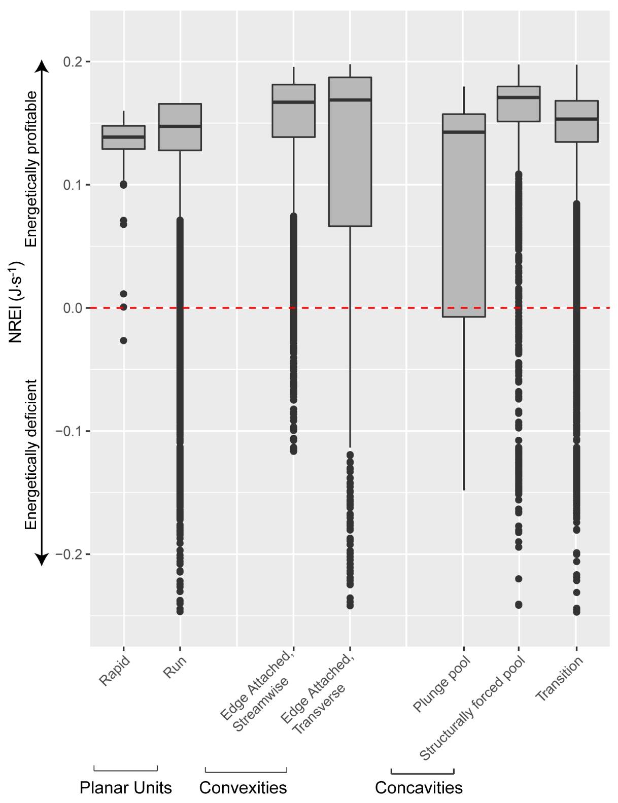
Figure B9. The distribution of NREI values within each geomorphic unit at Franklin Basin. The drift and temperature used were those collected during the snorkeling events: Drift 1.5 g.m3, temp 9.0° C.
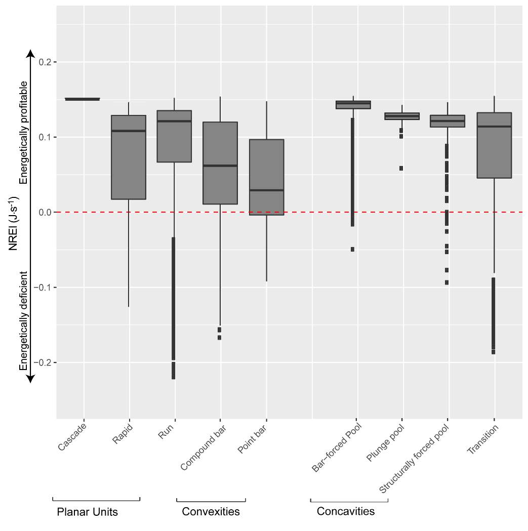
Figure B10. The distribution of NREI values within each geomorphic unit at Beaver Creek. The drift and temperature used were those collected during the snorkeling events: Drift 3.38 g.m3, temp 10.29° C.
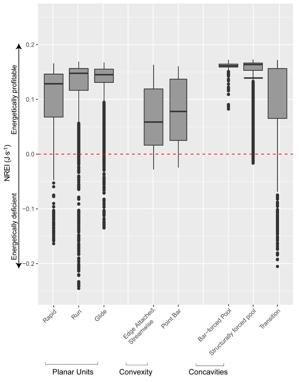
Overall, each site had a wide variety of convexities, concavities, and planar units. Notably, I wasn’t able to resolve the Tier 2 convexties, at all sites, to a Tier 3 classification. However, even resolved to Tier 2, there was a variety of edge-attached and channel-spanning convexities. Each site had at least two Tier 3 concavities and most sites had at least three types of concavities. Between the five sites, there was a wide variety of planar units, from glides to cascades.
NREI distributions within geomorphic signatures remained fairly consistent between the five physically diverse sites. Concavities, generally, had a higher median NREI value, than convexities, planar units, or transitions. This finding suggests that concavities may be the most energetically profitable areas in the stream, overall. This finding also suggest that their may be a bioenergetics signature for geomorphic units, especially concavities. However, since only 5 sites were used in this research, located within a single watershed, more research is needed across a wide variety of sites that encompasses a wide variety of physical attributes, habitat conditions, and riverine confinement.
Cite This Work
To export a reference to this article please select a referencing stye below:
Related Services
View all


Related Content
All TagsContent relating to: "Ecology"
Ecology is a field of biology that concentrates on the study of the relationships and interactions between living organisms (including humans) and their environments.
Related Articles

DMCA / Removal Request
If you are the original writer of this dissertation and no longer wish to have your work published on the UKDiss.com website then please: