Effects of Business Rankings on International Trade
Info: 11052 words (44 pages) Dissertation
Published: 2nd Nov 2021
Tagged: EconomicsInternational Business
1 INTRODUCTION
A customary promise in politics consists of “improving the business environment” or “promoting structural reforms” to help achieve greater wealth for society. Whether these promises are held to is beyond the scope of this dissertation; however, the indicators in which those promises are measured are. Popular and easy to understand rankings such as the World Bank Doing Business report receive considerable attention from the media, eager to show which countries have fallen or risen positions, year on year . Policy makers tend to pay attention to what international organizations’ indicators: “what matters get measured – and that what we measure is what ends up mattering” said UN Women Deputy Executive Director Policy and Programme John Hendra (2014) when talking about the UN Millennium Development Goals. But can these rankings accurately measure something as subjective as business friendliness? Moreover, and perhaps more importantly, does it really matter?
Examples of countries whose leaders-proclaim that they will promote business-friendly reforms are plenty (THE ECONOMIST, 2015). India ranked 142nd in the 2015 World Bank Doing Business Report, and its prime minister, Narendra Modi, pledged to propel it into the top 50. Rwanda, amidst plans of its president Paul Kagame to create a “Singapore of Central Africa” (THE ECONOMIST, 2012), ranked a remarkable 46th in the same report, but remains one of the poorest countries in the world. The anecdotal evidence seems mixed and it is still unclear on what scenarios these indexes can be reliable indicators of the reality.
I attempt to provide evidence of the effectiveness of these rankings through their effect on international trade. International trade is (perhaps surprisingly) a field that most economists agree upon and that it should be free (MANKIW, 2015). If improvements in these rankings can “lubricate” the cogs, or institutions, that also impact trade, we should expect a positive effect on welfare from this mechanism. Therefore, my specific research question is whether some of these rankings and reports influence a country’s trade flows through an empirical exploration of the gravity model of international trade.
The first hypothesis is that I will find a significant, positive interaction between a country’s exports and the quality of its institutions, these represented by a relevant indicator. This would indicate that improving the quality of institutions in a country would increase its trade flows. My second hypothesis is that these institutions interact more strongly with certain industries, and that specific indexes, when interacted with industry characteristics, will also have a positive effect on trade flows. This hypothesis stem from the fact that sectors are heterogeneous in the economy and may depend more or less on different institutions. Since the empirical results of the gravity model are well established, I expect that the refutation of the initial hypothesis would present evidence that these select indexes may not be the most adequate for guiding research and policy on the relationship between institutions and international trade. Thus, both possibilities are capable of providing meaningful results.
The dissertation relates to the articles on institutions as determinants of comparative advantage (NUNN; TREFLER, 2013) and the gravity model of trade (ANDERSON, 2010). It intends to provide a new perspective on the issue by analysing with the established methodology, models and variables of both literatures the applicability of the World Bank Doing Business indexes and some of its effects on international trade.
The rest of the dissertation is organized as follows. A background section introduces the past and current literature on the gravity model, institutions and how they relate in the field of international trade. The empirical model section details the model and data used in the empirical analysis and how it was manipulated to answer the research question. An ensuing analysis section presents the main findings and the final section summarizes the conclusions.
2 BACKGROUND
In this section, I first lay out the fundamentals in the literature of the two main components of this dissertation, the gravity model and institutions. I progress by linking these two components and presenting some contemporary studies. Finally, I present my own model for which I gathered data and estimated.
2.1 GRAVITY MODEL
The Gravity model of trade made its debut in economic debate through the seminal works of Tinbergen (1962) and has since been used by empirical economists for analysing flows of international trade. Named after an analogy with Newton’s universal law of gravitation, the “intuitive” model states that bilateral trade flows between countries is proportional to the size of their economies and inversely proportional to the distance between them, in a similar fashion as in equation (1).
Xab=(Sizea)α∙(Sizeb)β(costsab)γ
In which
Xab is the flow of the value of goods from country a to country b, Size measures the attracting “mass” of country a and b, costs are the total costs to trade between a and b. The main merit of the model is its strong empirical evidence. Several studies with different variables and methods find significant and consistent estimations according to the model. Even more so, the distance effect, measured as the elasticity of trade with respect to distance, is stable across numerous studies and is consistently around -1, at least since the 1970s (DISDIER; HEAD, 2008). The practical assumption was then is that distance increases transportation costs, and that transportation costs raise the price of the good in the importing country, leading to less trade.
One of the most fascinating debates derived from these empirical studies are the costs of national borders to trade, as initially shown in the United States-Canada border effects by McCallum (1995). His study showed that these two relatively similar countries in regards to culture, language and colonial origins, but separated by a border, can have vast differences from what a standard gravity model would predict in a borderless scenario. More specifically, he estimated that the trade flow amongst Canadian provinces is more than 22 times larger than the trade flow from a Canadian province to an American state. This showed compelling evidence against the widespread beliefs that globalization was making borders trivial, thus qualifying the effects of free trade agreements and economic integration processes and adding to contemporary debate.
These findings, however, lacked strong foundation in economic theory, raising questions about its validity. Its constant regularity seem to indicate there must be an underlying economic relation behind it, yet there was no consensus for the gravity model theoretical underpinnings. Anderson (1979) attempts to explain the phenomenon by deriving the gravity model from a Cobb-Douglas and a, in the appendix, a constant elasticity of substitution (CES) demand function, both in which countries produce and sell goods to other countries that are differentiated from the goods produced by the other countries. However, it had several limitations and did not fully explain the findings of the model.
It is only later that Anderson and Van Wincoop, (2003) elaborate the model that has become the benchmark for gravity analysis. They expand on Anderson’s CES model by showing that the flow of bilateral trade is affected by both the trade costs at the bilateral level (bilateral resistance) and the weight of these costs relative to all other countries (multilateral resistance). Their structural gravity model in a multi sector economy is represented by
Xijk=EikYikYktijkΠikPjk1-σk
Πik1-σk=∑jtijkPjk1-σkEjkYk
Pjk1-σk=∑itijkΠik1-σkYikYk
Where
Xijk is the flow of exports from country i to country j in product k,
Yik and
Eik are the value of production and expenditure in country I for product k,
Yk is the world output in sector k,
tijk are the trade costs of exporting a product k from country I to j and
σk is the elasticity of substitution among products.
Πik and
Pjk are the outward and inward multilateral resistances, respectively.
Intuitively, equation XX can be seen as two different parts: the left side of the equation or the “mass” term and the right side of the equation or the “cost” term. The mass term is the hypothetical level of frictionless trade between two partners in the absence of trade costs. In the overall equation, it means that large industries export more to the whole world, as large markets import from the whole world (ANDERSON, 2010). The cost term represents the trade costs that create the discrepancies between expected and actual trade. It is composed by the bilateral trade cost between partners I and j (traditionally estimated through geographic, political and policy variables), the outward multilateral resistance (country I ease of export) and the inward multilateral resistance (country j ease of import).
The main merits of this model is that it shows that changes in trade costs of one bilateral trade route influence the trade flows on the other trade routes because of relative prices. Since these resistances are by definition correlated with trade costs, so it improves on the basic intuitive model by eliminating the omitted variable bias that arises when failing to account for them. It is an empirical estimation of this model that the authors dispute about the magnitude of the border effects found by McCallum. Although their estimates were not as high, they nevertheless found a “border effect” between Canada and the United States that caused a reduction of 44% in trade flows.
In order to make it possible to estimate such a model, approaches in the literature (SHEPHERD, 2013) suggest using a fixed effects model transformation from equation XX
logXijk=logYik+logEjk-logYk+(1-σ)[logtijk-logΠik-logPjk]
To the equations XX:
logXijk=Ck+Fik+Fjk+1-σklogtijk
Ck= -logYk
Fik=logYik-logΠik
Fjk= logYjk-logPjk
Where
Ck is the constant that applies for all countries and is used as the proxy for the effect of the world’s production in sector k. The remaining terms are the exporter-sector and importer-sector fixed effects.
Other have also derived the gravity model from standard trade theory. Helpman et al. (2008) and Bergstrand (1985) presented a models of the gravity equation based on the assumption that firms are heterogenous in productivity. Deardoff (1998) derived the model based on the Hecksher-Ohlin model of international trade, in which countries have different factor endowments, and Eaton and Kortum (2002) derived the model out of the Ricardian model, in which countries vary in technology. While these models have their merits, I focus on that from Anderson and Van Wincoop (2003) because of its simplicity and its ease of estimation.
Most of the literature consist of trying to devise better estimates for the trade costs. These have been subject of much study since Linnemann (1966) categorized them into shipping costs, time-related costs and cultural unfamiliarity, this last being of particular importance. Anderson and Van Wincoop (2004) show through empirical observations using their model that several variables have a significant effect on trade through the increase or decrease of trade costs and that are well beyond those variables that are observable.
Shipping costs are the most apparent; its weight in the final cost of exported goods vary a great deal according to the distance of the two countries and the nature of the goods being transported[1]. Anecdotally, it should not be a surprise that it costs less to export jewellery from Switzerland to Germany than it does to export coal from Australia to the United Kingdom. These costs have fallen significantly in the era of globalization mainly due to technological changes, such as the containerization and jet aircraft engines, and economies of scale in the shipping industry (HUMMELS, 2007).
Time-related costs are relevant because of the time value of the money, the perishability of products and the constraints of a significant lag between ordering a shipment and receiving the products, all of which can affect a firm’s to export or import. Payment terms to the importer can range from full payment before production to full payment several months after the shipment, depending on the assessment of risk of the transaction by the partners. Products such as fresh fruit or flowers require complex coordination so they can reach their markets when they are the most adequate for consumption. Finally, some industries, such as fashion retailing, may see the boom and the bust of a trend in less time than it takes a cargo freighter to arrive from the traditional producers in Asia.
The cultural unfamiliarity costs present a different challenge, as they are not as easily observable as shipping costs or time related costs. A more intuitive systematization of such costs is the CAGE distance framework by Ghemawat (2001) and presented in Table 1. The framework lists the cultural, administrative, geographic and economic differences among countries. Intended as a guide for companies interacting with foreign markets, it nevertheless succeeds in systematizing the variables of interest for calculating the trade costs across countries, many of which have been empirically tested before and after its inception.
Table 1 – CAGE distance framework
| Cultural Distance | Administrative Distance | Geographic Distance | Economic Distance |
| Different Languages
Different ethnicities; lack of connective or social networks Different religions Different social norms |
Absence of colonial ties
Absence of shared monetary or political association Political hostility Government policies Institutional weakness |
Physical remoteness
Lack of a common border Lack of sea or river access Size of country Weak transportation or communication links Differences in climates |
Differences in consumer incomes
Differences in costs and quality of: -Natural resources -Finance resources -Human resources -Infrastructure -Intermediate outputs -Information or knowledge |
Source: adaptation from Gemawat (2001), page 5
Because of the existence of these cultural unfamiliarity costs and other geographical distance costs that are not captured solely by the geodesic distance between two countries, economists add several more observable variables to their models as proxies to control for such effects in the gravity model. Geographic distance dummies include if the countries share common borders or if they are landlocked, for instance. Common language is the most usual proxy for the cultural distance, as it is very intuitive that sharing a language should reduce the friction in trade. Other studies use less common variables for proxying cultural distance, such as having a common religion or if they were ever the same country.
The category that interests economists the most is the administrative distance because of its actionable policy implications. If a country has had a common colonizer or was colonized by its partner, then the effect on trade due to lessened cultural and administrative differences should be lessened. That effect is observed empirically (KLEIMAN, 1976), but Head et al. (2010) finds that trade after four decades reduces by significantly between the independent country and its colonizer and former colonies of the same empire, suggesting this variable also changes over time. Tariffs are also considered administrative costs and act directly on the price of the good, thus increasing the trade costs from country I to country j of product k and can also be included in the model.
Economic integration also seems to be a powerful policy to reduce trade costs. In an extensive study of regional blocs, Frankel et al (1997) uses the gravity model to test a set of hypothesis on such agreements, including the size of the influence they have on trade flows. His results suggest there is a positive effect of economic integration. A similar study is conducted by Baier and Bergstrand (2007) on the effect of free trade agreements, and they also find a positive effects on trade flows. Subramanian and Wei (2007) study the effect of WTO membership and show that it also has had a positive effect on trade, but largely uneven, increasing disproportionately the developed countries’ imports in relation to their exports.
Knowing the limitations of using only geodesic distance to estimate trade costs, the literature tends to estimate the trade cost term in the gravity model as
logtij=β1logdistanceij+∑m=1Mβmlog(cost_variableijm)
Where the dependent variables include the geodesic distance between economies and a series of M selected terms that try to capture the remainder of the trade costs between the pair. The distance is usually interpreted as a proxy for shipping costs, and the other variables tend to be selected to act as proxies the intangible aspects of trade costs. These consist of some of the more stablished indicators, such as having a common language, sharing borders or having a similar colonial past. Other variables tend to be related to trade policy and analyse the effect of those, such as the magnitude of tariffs or participating in a Regional Trade Agreement (RTA). Finally, empirical researchers add their variable of interest to this term expecting to find a significant coefficient.
Since then, most economists agree that the empirical regularity of the gravity model makes it a valid field of research, and there have been significant improvements to the original model. Some contributions to the model focus on its correct specification and how to estimate it more precisely. There are two nearly standard practices when estimating the standard errors in the gravity model: robust and clustered errors (SHEPHERD, 2013). The robust estimation is an effective way of fixing heteroskedasticity, and the clustering of errors by country pairs allows for correlation among them, avoiding the error of understating errors in data with multiple levels of aggregation (MOULTON, 1990). They are both measures that increase the standard error of estimations, turning any estimations more conservative and reliable.
Silva and Tenreyro (2006) argue that the practice of using ordinary least squares (OLS) to estimate log-linear models is flawed because it leads to biased estimates of the true coefficients and their standard errors under heteroskedasticity. They argue for the use of the Poisson pseudo-maximum likelihood estimator (PPML), as its properties allow for both the treatment of the heteroskedasticity and the prevalence of zeros in gravity datasets, while still maintaining important characteristics of the OLS estimators, such as the consistency in the presence of fixed effects and simple interpretation.
A problem that arises with the comparison with Newton’s equation is that, unlike the positive yet possibly very small values predicted by it, trade flows contains several zeros among country pairs. Common sense indicates that it would not surprising that East Timor did not trade with Swaziland in a given year, but it presents challenges for the correct usage and interpretation of the model. The most common approach is to omit any zero pairs from the analysis, as the log of zero is minus infinity. This might bias the results due to sample selection, but studies do not entirely agree on the severity of such bias and on how to handle it. Helpman et al. (2008) propose an explanation for the zeros found in the data through the fixed costs to export that monopolistic competitive firms face. If no is firm productive enough in country I to export to country j, then there would be zero trade flows between the two economies.
Other applications of the model have shown the extensiveness of its usefulness to a variety of fields that deal with country flows. The use of gravity models for migration flows dates from before its usage in international trade with Ravenstein (1885)and has had recent developments with Helliwell (1997), showing that immigration is curbed even more than trade by the United States-Canada border. Gravity models have also been shown significance when estimating equity flows between countries (PORTES; REY, 2005), even though apparently the distance variable does not have a direct effect on such flows. In this case, the distance serves as a proxy for information costs. In a similar spirit, the gravity model has also been used in estimating foreign direct investment flows (BRENTON; DI MAURO; LÜCKE, 1999).
Even with its recent developments and use, the gravity model is far from achieving unanimous consensus on its specifications, methods and data. It nevertheless retains the properties of strong empirical evidence and, with the Anderson and Van Wincoop (2003) framework, it has evolved into an useful tool for trade policy analysis in a multi-country environment (YOTOV et al., 2016).
2.2 INSTITUTIONS
Institutions are very difficult to define. Most researchers interested in studying the economic impact of institutions tend gravitate towards the notion that institutions are “the rules of the game in a society, or, more formally, are the humanly devised constraints that shape human interaction” as stated by North (1990). Although there confusion in trying to define such a difficult concept, institutions are easily illustrated; North (1990) suggests the exercise of trying to make the same transaction in a different country to observe their difference.
Institutions matter because they change the incentives of agents: “Our (individuals) opportunities and prospects depend crucially on what institutions exist and how they function” (SEN, 1999). Acemoglu and Robinson (2013) argue that institutions are the main reasons to a nation’s economic prosperity. According to the authors, countries become wealthy because they cultivate inclusive institutions rather than extractive institutions. That means that the institutions in these countries “include” the interests of the population by protecting private property and enforcing contract law rather than “extract” the wealth for the privilege of an elite by creating mechanisms to unequally transfer resources. Since institutions tend to persist across time (ACEMOGLU; JOHNSON; ROBINSON, 2000), extractive institutions can perpetuate a vicious cycle of poverty, as can inclusive institutions perpetuate a virtuous cycle of prosperity. Other authors emphasize the role of legal origins in originating a country’s institutions and how these affect institutions that, subsequently, affect current economic performance (LA PORTA; LOPEZ-DE-SILANES; SHLEIFER, 2008).
Given the importance of the study of institutions to economic prosperity, it has led to the development and publication of several indexes that aim to give a more tangible data for the study of this subject. For instance, the Transparency International Corruption Perception Index (TRANSPARENCY INTERNATIONAL, 2015) condenses in a single number the perception of government corruption for each country. It is calculated using several data sources from other independent institutions on the perceptions of business people and risk analysts of the corruption ingrained in the country. Although at first glance a single number might appear overly simplistic, the index shows strong correlation with two other measures of corruption, black market activity and overabundance of regulation, indicating its validity (WILHELM, 2002).
Particularly notable and more useful to my research is the World Bank Doing Business report (WORLD BANK, 2017). Published since 2004, it has been since one of the World Bank’s flagship reports. It is based on the notion that clear and sensible rules influence economic activity in a positive and meaningful way. Therefore, it provides quantitative indicators about several regulatory dimensions and how well (or not) they fit into the ideal scenario of efficient, simple and accessible regulation that promotes social welfare. The economies that receive the highest scores are not necessarily the ones that have the least regulation, but rather take a risk-based approach to it (regulating more heavily the more risk to the population an activity poses) and facilitate market interactions without needlessly hindering the private sector. In this sense, the Doing Business relates to the inclusive economic institutions by Acemoglu and Robinson (2013) as a vehicle of prosperity.
However, rankings and scores like these are far from perfect. Høyland et al. (2012) criticize rankings for being presented as highly precise despite the inherent impreciseness introduced by high levels of noise in their calculation. Furthermore, they also argue that it incentivizes rank-seeking behaviour rather than policies that actually improve underlying institutions. Rankings makes it easier for autocrat governments to make short-term cosmetic gains in rankings and scores, even when these changes are not meaningful for the economy as a whole and meant to disguise the country’s real standing.
Despite of the Doing Business’ qualities, it also faces considerable criticism. The report is consistent with public choice view that suggests that regulation is devised for the benefit of politicians and government officials, rather than for the country (SHLEIFER; VISHNY, 2002). Arruñada (2007) dispute those claims and argue that while some degree of rent-seeking may be observable and should be combated, regulation should not be oversimplified because of the possible benefits from it. The report also acknowledges that because of its reliance on formal regulation, it does not always accurately captures all factors in that affect a country’s actual business environment (WORLD BANK, 2017). Some countries that strangely appear as bottom performers may be so because its regulation is extremely strict, but their de facto rules are less so because of corruption (where bribery can be the norm for most business practices) or a light enforcement of the law.
That said, hardly any index will ever be able to fully grasp the complexity of such subjective measure such as institutions. The Doing Business report is relevant because of its reach and importance attributed to it by rulers, investors and policy makers and is backed by the World Bank, an international organization that enjoys considerable prestige. Moreover, it is one of the richest reports in terms of data, both in its disaggregation into multiple indicator sets (10) and in its coverage of countries (190 economies). Therefore, I choose to focus mainly on this report to give relevance to my analysis.
2.3 THE LINK
In this section, I discuss how institutions relate to international trade and the gravity model. As Nunn and Trefler (2013) note, studies on the field suggest that institutions play an important role as determinants of trade and much bigger than through an indirect effect on factor accumulation or technological innovation. Indeed, poor (good) institutions in a country can be seen as a cost (discount) factor for the exporter firms, decreasing (increasing) the amount of goods exported and the country’s trade flows. This observation relates to my first hypothesis that countries with better institutions trade more.
Academic research has shown evidence that institutions and international trade are significantly related using a variety of ways and research data (ANDERSON; MARCOUILLER, 2002; CHOR, 2010). Nunn and Trefler (2013) provide a comprehensive review of the subject. I choose to highlight the studies that show the interaction of institutions and international trade through different industry characteristics, as they relate to my second hypothesis: some institutions matter more for specific industries. I incorporate their insights to my specific model in section 3.
Assume a model of incomplete contracts, in which the input supplier produces a customized good for the end-product firm as in Cabral (2017). Because of this customization, the input is of greater value to the end-product firm than to other buyers. Investments made by the supplier are said to be relationship-specific. Because of incomplete contracts and imperfect enforcement, there are incentives to deviate from it, creating the hold-up problem. This causes a undesirably low relationship-specific investment and creates inefficiency in production. Making an analogy to international trade, such as the general equilibrium model by Levchenko (2007), the implication is that countries with better institutions to enforce these incomplete contracts will have a comparative advantage in the sectors that are most affected by the hold-up problem.
In that context, Nunn (2007) builds an index of how dependant an industry may be on contracts, or its “contract intensity”. Nunn begins with Rauch’s (1999) classification of product heterogeneity, which classifies products whether they are sold in organized exchanges (commodities), reference priced (catalogues) or are differentiated (neither trades on exchanges or appears in catalogues). His interpretation is that if the product is classified as differentiated, it is subject to the hold-up problem, while the others are not. He crosses the classification with data from the US input-output matrix to calculate the “contract intensity” of goods. Assuming that the US contract dependence of industry k is the closest to a frictionless measure of such index and that it is valid for every country I, he constructs his empirical test in the form of:
Xik=αi+αk+βzk∙qi+Xik+εgi
Where
Xij is the exports from country I in product k,
αi and
αk represent fixed effects for the country and industry,
zk is the contract dependence variable of industry k,
qi is a measure of contract institutional quality on country I and
Xik is a vector of other determinants of comparative advantage. The model suggests that
β>0, and Nunn’s empirical results confirm that hypothesis.
Rajan and Zingales (1996) study the contribution to industry output from the interaction between industry’s sensitivity to credit and countries’ financial development. For that, they define an important variable, the external finance dependence, em, as the fraction of a firm’s capital structure that is financed from sources external to the firm. This relation is shown below.
em≡capital expenditures-(cash flow from operations)(capital expenditure)
They assume that industries have technological differences that require different levels of cash and finance at different times, and calculate the index for whole industries too. They also extrapolate their index from the industries in the US to the whole world, assuming that would be the desirable external finance level in a financially frictionless economy. They interact this term with measures of financial development per country and find a positive and significant relation. Their methodology can be easily translated to the international trade literature, as in equation XX:
Xik=αi+αk+βek∙fi+Xik+εgi
Where the terms are the same as in equation XX, but the interaction variable is the external finance dependence, ek, times a measure of the countries’ finance development, fi. This presents an interesting view on the interaction of financial institutions and international trade, but the literature has noted that it is likely to suffer from endogeneity, it is likely that there are omitted country level factors that interact with industrial structure and financial institutions. Manova (2008) for instance, tackles this problem by analysing the interaction before and after there is a trade liberalization. Overall, there is still room for advances in the subject.
Cuñat and Melitz (2012) examine the relation between a country’s labour institutions and international trade. Based on a model with a “rigid” and a “flexible” economy, they predict that in the presence of firm-level shocks, more flexible countries are able to reallocate their labour across firm more easily, thus generating increased productivity in the industries more susceptible to these shocks and becoming a source of comparative advantage in the Ricardian notion. They use sales data from publicly traded firms in the United States to create an “industry volatility” index and indentify the industries that are more susceptible to shocks. This measure is then multiplied by a country-specific measure of labour flexibility in equation XX:
Xik=αi+αk+βvk∙li+Xik+εgi
Where the terms are the same as in equation XX, but the interaction variable is the sales volatility index,
vk, times a measure of the country’s labour flexibility,
li. As expected, the
β estimated by the authors is positive even when controlling for other traditional comparative advantage predictions.
This body of research presents interesting insights on how institutions can interact with different indexes in order to affect international trade. Using the gravity model’s desirable properties for empirical testing, I choose to use it as a tool for testing hypotheses about these interactions. The focus, however, is to adapt their variables to fit my model using the World Bank Doing Business reports as measures of institutional quality. I progress in the next chapter by creating this model.
3 EMPIRICAL MODEL
In order to estimate a gravity model equation and answer the research question I propose, I take a few different approaches to it. First, I define my distance variable as
logtijk=β1logdistanceij+β2contiguityij+β3 comlangij+β4 comcolij+β5 colonyij+β6 FTAij+β7 Fk
It includes the weighted geodesic distance of two countries
(distanceij) and the dummies for observable characteristics of distance of shared borders (contiguityij), common language (comlangij), common colonizer past 1945 (comcolij), ever in a colonial relationship (colonyij) and free trade agreements (FTAij) and a fixed effects vector to account for industry variation (Fk). Then I include it in the “intuitive” gravity model equation alongside the institutional quality variable (Institutionsi,t). This combination takes the basic form of equation (X):
Xij,tk=α0+β1logGDPi,t+β2logGDPj,t+β3logtijk+β4Institutionsi,t+ εijk
The dependent variable is
Xij,tk is the log of exports from country I to country j to in the 4-digit SIC industry k in year i. The independent variables are the model’s constant (α0), the natural logarithms of each countries’ GDP in year t (
GDPi,t and
GDPj,t). The coefficient that will provide meaningful information for my main hypothesis is the β3, its significance and economic relevance. A positive effect means that a better overall score in the score of the quality of the institutions has a positive impact on trade flows.
To test my second hypothesis, that some sectors in the industry react differently to the quality of different aspects of a country’s institutions, I add to this preliminary equation the interaction effects mentioned in section 2.3 and displayed in equation (X):
β5zk∙qi+β6ek∙fi+β7vk∙li
A positive effect to these coefficients would mean that trade flows respond to the interactions between institutions and industry characteristics tested.
I then proceed to estimate the gravity model inspired by Anderson and Van Wincoop (2003) in equation XX.
Because of the lack of available data by sectors (the k in the equation), I choose to follow a simpler version of the model, without the sector variables.
logXij=C+Fi+Fj+1-σlogtij
C= -logY
Fi=logYi-logΠi
Fj= logYj-logPj
Finally, I add the discussed institutional variables.
I therefore aim to estimate the equation XX, that incorporates the gravity variables, controls and proposed variables for analysis:
Xijk=α0+αiyi+αjyj+Xi+Xk+ εijk
The usage of data over time transforms the model from a cross-sectional regression into a panel regression. This is desirable because it controls for heterogeneity among countries, makes it possible to identify specific time or country effects and avoids the potential multicollinearity of cross-section data.
3.1 DATA
In this section, I describe the data I gathered and the manipulations necessary to fit it into a cohesive dataset necessary to perform the estimations of my model. I cite sources and exemplify conversions. Clarifications on specific methods are available upon request.
The starting point in gathering the necessary data is finding the adequate trade flows. Countries report their trade data in the Harmonized System, a 6-digit code that is used to classify the different types of merchandise trade among countries. While some countries and economic blocs use more disaggregated classifications for internal purposes (such as the US 10 digit HS or the Mercosur 8 digit NCM), they are all built upon the 6 digit HS and are reported as such to the related United Nations (UN) Statistics Division and store in the UN Commodity Trade (Comtrade) database. In order to convert this important product data into a common industry classification, I used the World Integrated Trade Solution (WITS), a software that allows users to download the Comtrade data in several industry classifications. I chose the 4 digit Standard Industry Classification (SIC), a classification formerly used by the United States and in which to the remaining data can be converted to with the least steps, in order to minimize data distortion.
I focus on export flows, in sync with the derived model in XX. It is also analogous to the competitive advantage literature that has already yielded interesting results of the relation of institutions and trade flows. Due to the nature of these aggregate trade flows, there are several observations that are zero or close to it (less than 1000 USD in a given year and SIC industry), and, therefore, are not included in the dataset. This approach is the most commonly utilized by the related literature cited in the previous section, thus replicating it makes using such data more meaningful. It also gives the further meaning to the coefficient estimates that they must be understood in condition to having positive flows from country a to b. The period of analysis is from 2007 to 2015, a recent period that has plenty of data availability for all variables in the model.
The loss of refinement due to the usage of an older industry classification (SIC) is not critical to this dissertation. My trade data consists of transactions of products among economies, and newer classifications and revisions have been created to picture the evolution in services more clearly. Furthermore, new classifications are also created to be highly compatible with previous ones to minimize the impact of changing standards or converting data.
The variables used in the traditional gravity model and the relevant controls come from the CEPII database (HEAD; MAYER, 2013). It provides country-pair information per year and several dummies for specific characteristics. Based on the review resent in the previous section, the variables I use from the dataset are the GDP of the economies, the distance between country pairs and the dummies for contiguity, common language, common colonizer, colonial relationship and presence of free trade agreements. The GDP is reported in nominal terms, converted to US dollars, as is required by the gravity model proposed that deflates the value through the two resistance terms. The variable for distance in the dataset does not constitute of the distance between capitals, but rather the weighted distance between the biggest city of the two countries, accounting for intra-national distances (MAYER; ZIGNAGO, 2011). This corrects for some biases, especially in large countries, where the capital does not solely represents the biggest or most relevant economic area and there is considerable “distance” within the same country. The dataset, does not, however, have data for all country pairs, but most that are left out are either recently formed countries (i.e. South Sudan) or very small nations and territories (i.e. Aruba), thus not presenting significant systematic errors to the estimation.
The data on the dependence on contracts comes from Nunn (2007). His industry classification is the 6-digit input-output classification of the United States Bureau of Economic Analysis (BEA) in 1997, a similar classification to the North American Industry Classification System (NAICS), which, in turn, is a more modern version of SIC. To convert the data to SIC, I have used the BEA’s guidelines (STEWART; STONE; STREITWIESER, 2007) to convert the I-O to NAICS (1997 revision), and then used the US census concordance tables (US CENSUS BUREAU, [s.d.]) to convert it to the SIC classification. Because of some inherent discrepancies between the different classifications, I took some measures to make the data comparable. When converting from the BEA I-O classification to NAICS-97, some unique classifications corresponded to several unique ones. In these cases, I assigned the index calculated by Nunn for the broader category to all correspondent categories (see Table 2 for examples). No other conflicts ensued because the 1997 BEA’s I-O classification was created based on the NAICS.
Table 2 – BEA I-O to NAICS examples
| I-O | Description | NAICS | Description |
| 1111A0 | Oilseed farming | 11111 | Soybean farming |
| 11112 | Oilseed (except Soybean) farming | ||
| 335110 | Electric lamp bulb and part manufacturing | 33511 | Electric Lamp Bulb and Part Manufacturing |
| 335120 | Lighting fixture manufacturing | 335121 | Residential Electric Lighting Fixture Manufacturing |
| 335129 | Other Lighting Equipment Manufacturing |
Source: Own elaboration based on Stewart et al. (2007)
This method did not differ greatly when assigning correspondent industries from NAICS-97 to SIC. Some SIC categories had only direct correspondence with sub categories of NAICS (that is, 6 digit instead of 5 digit) that did not have a direct correspondence with the previous BEA I-O classification. In these cases, I assumed the ramifications of the category had the same Index as their parent node much like in Table 2. In the end, Nunn’s 381 sectors corresponded to 441 unique SIC codes after discarding those values that corresponded to services and construction and that are not present in the trade data.
The data for external finance dependence, as it was built by Rajan and Zingales (1996) was gathered from publicly traded companies on Compustat through the Wharton Research Data Services (WRDS). With data from 1980, I used their methodology to construct the cash flow from operations with the items reported by the US companies for each year. From the years of 1980 until 1987, cash flow from operations was a single entry in Compustat (FOPT). From then on, it was calculated differently[2], but a few firms have the data in both forms for the year of 1987 and it is rigorously the same as the previous entry, which indicates the validity of the calculation. I then merge both variables to create a single cash flow from operations variable, valid for all years from 1980 to 2015. Capital expenditures is considered a single entry (XXX) throughout the whole period.
A more complex issue arises when building calculating the external finance dependence index as described in the previous section. Each company is classified by the US Securities and Exchange Commission (SEC) in a modified 4 digit SIC code that resembles the 3 digit SIC code with some added 4 digit SIC categories. This creates a larger number of industry categories in which companies are classified than in the original paper, reducing the number of companies per industry code and possibly creating unreliable numbers if only the period proposed in the article (one decade) is used. To decide which time frame I should use, I construct the index using the average capital expenditures and cash flow from operations for each company in the shorter, relevant of period of 2006 to 2015 and in the longer period of 1980 to 2015. I then take the median of the values in all industry codes that have more than two companies to create the index.
The indexes from both periods are highly correlated (0.9095). However, not only the magnitude of the values obtained in the longer period more closely resemble those found by Rajan and Zingales, but also there are more industry codes with more than 2 companies to obtain the median. I choose to proceed with the index obtained from the longer period. Table 3 compares the five biggest values and the five lowest values calculates by Rajan and Zingales in the 1980’s using ISIC industry classification and the equivalents in my own calculations from 1980 to 2015 using the SIC industry classification.
Table 3 – external financing accross industries
| ISIC code | ISIC industry | Rajan Zingales | SIC code | SIC industry | My own calculations |
| 314 | Tobacco | -0.45 | 2111 | Cigarettes | -4.25 |
| 361 | Pottery | -0.15 | 3269 | Pottery producs, NEC | -0.46 |
| 323 | Leather | -0.14 | 3111 | Leather goods, NEC | -1.84 |
| 3211 | Spinning | -0.09 | 2281 | Yarn spinning mills | -0.20 |
| 324 | Footwear | -0,08 | 3149 | Footwear except rubber | -1.28 |
| 385 | Professional goods | 0.96 | 3826 | Laboratory instruments | 0.93 |
| 3832 | Radio | 1.04 | 3663 | Radio and TV equipment | 0.46 |
| 3825 | Office and Computing | 1.06 | 3571 | Electronic computers | 0.72 |
| 356 | Plastic products | 1.14 | 2673 | Plastic bags | 0.45 |
| 3522 | Drugs | 1.49 | 2834 | Pharmaceutical preparations | 6.29 |
Source: own elaboration with data from Rajan and Zingales (1996) and Compustat.
The data for sales volatility used by Cuñat and Melitz (2012) also comes from Compustat and WRDS, but their methodology presents the opposite challenge, by being very strict on its parameters and possibly leading to an excessive cleaning of a data so disaggregated as that of the 4 digit SEC SIC. In order to create a significant and conservative index, I choose to follow their steps and use only companies with at least ten years of data and industries with at least five companies listed in the period of 1980 to 2015. I calculate the year on year log differentiated sales of the companies and the average employment over time. I then proceed to create the industry sales volatility index by merging each company’s sales volatility weighted by their industry employment.
There is no formal conversion table from the SEC SIC to the regular SIC. In order to merge the industry variables calculated from Compustat (sales volatility and external finance dependence) I used SEC SIC codes that had the same description as the 3 digit SIC code to all 4 digit SIC codes that did not have a specific correspondence in the SEC SIC. This allows for the indexes derived from Compustat to be merged correctly to the trade data. Table 4illustrates a few clarifying conversions.
Table 4 – SEC SIC to SIC conversion
| SEC SIC | Description | SIC | Description |
| 2870 | Agricultural chemicals | 2873 | Nitrogenous fertilizers |
| 2874 | Phosphatic fertilizers | ||
| 2879 | Pesticides and Agricultural Chemicals, NEC | ||
| 3080 | Miscellaneous plastic products | 3082 | Unsupported plastics profile shapes |
| 3081 | Unsupported plastics film and sheets | 3081 | Unsupported plastics film and sheets |
Source: Own elaboration.
Given my specific interest in the World Bank’s Doing Business reports, I gathered the data on countries’ institutions directly through its reports and available datasets. Their data present a number of positive points. First, there is data for several countries and territories in the world, including the ones with reported trade data. Second, they publish a simple and easily comparable “distance to frontier” score for every country in every subdivision of the report. This number, theoretically ranging from 0 to 100, shows how close a country is to the frontier (best practices) in that category and in the overall doing business practices.
The Doing Business has several subdivisions of interest. Chosen through the World Bank Enterprise Surveys with data from more than 130,000 entrepreneurs in 139 economies, they are: starting a business, dealing with construction permits, getting electricity, registering property, getting credit, protecting minority investors, paying taxes, trading across borders, enforcing contracts, resolving insolvency and labour market regulation (WORLD BANK, 2017). Only a few are of direct interest to this dissertation:
- Overall or “ease of doing business”: and indicator of the country’s overall position in promoting a friendly business environment through regulation. This is measured as a simple average of the distance to frontier of all the other indicators. Because of its comprehensiveness, it is the indicator used for the ranking in the report.
- Trading across borders: indicates how institutions in a country curb or encourage trade. It measures specifically the time and costs of the logistical process associated with exporting and importing goods.
- Enforcing contracts: indicates the time and cost of commercial disputes and the quality of the judicial processes. It measures through a hypothetical commercial litigation between two domestic businesses: a seller sues the buyer for not accepting a shipment of custom goods, which the buyer deems of poor quality. Because of its incomplete contracts dimension, I use it as the indicator of rule of law to reproduce the interaction in Nunn (2007).
- Getting credit: indicates the efficacy of movable collateral laws and credit information systems in facilitating access to credit. It measures the (1) legal rights of borrowers and lenders through collateral and bankruptcy laws that facilitate lending and (2) the credit information through its availability and quality. I use it as the indicator of a country’s financial institutions to reproduce the interaction in Rajan and Zingales (1996).
- Labour market regulation: indicates the flexibility in employment regulation and job quality. The data comprises information on the country’s labour laws that relates to these two dimensions such as hiring, working hours and redundancy costs.
Under criticism, the labour flexibility’s distance to frontier and ranking are not published since 2005. The study that originated the World Bank’s methodology by Botero et al. (2004) shows that heavier regulation of labour is associated with lower labour force participation and higher unemployment, thus inspiring the inclusion of an index that measured labour regulation. Critics have pointed out that the sub index discourages countries from maintaining high enough levels of labour regulation desired by society (BAKVIS, 2006) and some of inconsistencies with recent trends in the regulation of developed countries, such as the length of working hours (MESSENGER; LEE; MCCANN, 2007). This exemplifies how difficult it can be to measure accurately institutions.
Because the raw data on the indicator is still gathered. The Heritage Foundation, an American think tank, uses the World Bank data for the construction a similar sub index called Labour Freedom, part of a broader Economic Freedom index (THE HERITAGE FOUNDATION, 2016). The Labour Freedom maintains the spirit of the original World Bank index by using the same three quantitative factors (difficulty of firing, rigidity of hours and difficulty of firing redundant workers) while adding three more (Ratio of minimum wage to the average value added per worker, Legally mandated notice period, Mandatory severance pay). These six factors are all equally weighted to form a score that ranges from 0 to 100, which facilitates comparisons and interpretations. Therefore, I use it as the indicator of labour flexibility to reproduce the variable in Cuñat and Melitz (2012).
The final dataset contained 13,467,567 observations of trade flows in 9 years of data from 162 exporting countries to 191 importing countries in 440 unique SIC codes. Table 5 shows some descriptive statistics of some of the variables of interest to the model.
Table 5 – Descriptive statistics of model variables
| Contract dependence | External finance dependence | Sales volatility | |
| Mean | 0,5322 | -0,1046 | 0,1839 |
| Standard deviation | 0,2022 | 1,6657 | 0,0549 |
| Maximum | 0,9562 | 22,8644 | 0,3476 |
| Minimum | 0,0242 | -4,2488 | 0,0898 |
Source: Own elaboration with data from Nunn (2007) and Compustat.
4 ANALYSIS AND RESULTS
In this section, I present the results of the estimation of the proposed model. I also discuss its interpretation and some of its limitations.
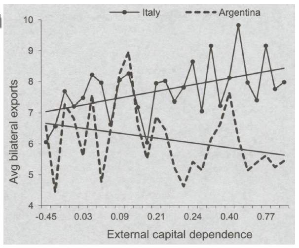
Preliminary results show that… For instance, the relationship of country X and Y can be seen in the graph below.
Following the reasoning in section 3, I present the results of the intuitive regressions in Table 6. All regressions uses clustered errors by country pair (distance).
Table 6 – Intuitive model
| (1) | (2) | (3) | (4) | |
| GDP Exporter | 0,8591 | 0,8523 | 0,9355 | 0,9483 |
| 0,0082 | 0,0091 | 0,0099 | 0,0097 | |
| GDP Importer | 0,5241 | 0,5312 | 0,5846 | 0,5982 |
| 0,0067 | 0,0068 | 0,0076 | 0,0076 | |
| Weighted distance | -0,7699 | -0,7848 | -0,8983 | -0,9157 |
| 0,0196 | 0,1971 | 0,0212 | 0,0213 | |
| Doing Business distance to frontier | – | 0,0056 | 0,0056 | 0,0015 |
| 0,0013 | 0,0014 | 0,0019 | ||
| Relation Specificity X Contract Enforcement DTF | – | – | 0,0152 | |
| 0,0023 | ||||
| External Finance Dependence X Getting Credit DTF | – | – | 0,0018 | |
| 0,0001 | ||||
| Sales Volatility X Labour Flexibility | – | – | -0,0049 | |
| 0,0044 | ||||
| Constant | -26,2554 | -26,5956 | -28,2221 | -28,6872 |
| 0,3357 | 0,3317 | 0,3884 | 0,3840 | |
| Gravity controls | Yes | Yes | Yes | Yes |
| Exporter/Importer country fixed effects | No | No | No | No |
| Industry fixed effects | No | No | Yes | Yes |
| Year fixed effects | No | No | No | No |
| R² | 0,2544 | 0,2515 | 0,3621 | 0,3714 |
| Number of observations | 13467567 | 9393798 | 9393798 | 7202240 |
| Number of clusters | 22705 | 21746 | 21746 | 21037 |
Notes: dependant variable is the log of exports from exporter country i to importer j in the SIC industry m in the year 2015. GDP Exporter, GDP Exporter, Weighted Distance are all measured in log terms. ** and *** denote statistical significance at the 5 and 1 percent levels, respectively. Gravity controls represented by dummy variables are contiguity, common official language, common colonizer (post 1945) and if the pair is in a regional trading agreement. The robust standard errors clustered by country pair estimated are shown in brackets.
The effect of XYZ is highly statistically and economically relevant.
Second stage of the analysis: to reduce the omitted variable bias, we further the analysis by including industry specific indicators. Those are based on prior research and include …
These results are shown in Table 7.
Table 7 – Fixed effects model
| (1) | (2) | (3) | (4) | |
| Weighted distance | -1,2076 | -1,2354 | -1,2219 | -1,2451 |
| 0,0221 | 0,0221 | 0,0221 | 0,0222 | |
| Average Doing Business distance to frontier | – | – | 0,0046** | -0,0041 |
| 0,0018 | 0,0018 | |||
| Relation Specificity X Contract Enforcement DTF | – | 0,0449 | – | 0,0445 |
| 00016 | 0,0016 | |||
| External Finance Dependence X Getting Credit DTF | – | 0,0019 | – | 0,0019 |
| 0,0000 | 0,0000 | |||
| Sales Volatility X Labour Flexibility | – | 0,0308 | – | 0,0301 |
| 0,0019 | 0,0022 | |||
| Constant | 6,3120 | 17,0172 | 17,6586 | 18,1507 |
| 0,4427 | 0,3748 | 0,4021 | 0,3907 | |
| Gravity controls | Yes | Yes | Yes | Yes |
| Exporter/Importer country fixed effects | Yes | Yes | Yes | Yes |
| Industry fixed effects | Yes | Yes | Yes | Yes |
| Year fixed effects | Yes | Yes | Yes | Yes |
| R² | 0,4178 | 0,4297 | 0,4177 | 0,4272 |
| Number of observations | 13467567 | 10187199 | 9068998 | 6952074 |
| Number of clusters | 22705 | 21579 | 20707 | 20034 |
Notes: dependant variable is the log of exports from exporter country i to importer j in the SIC industry m in the year 2015. GDP Exporter, GDP Exporter, Weighted Distance are all measured in log terms. ** and *** denote statistical significance at the 5 and 1 percent levels, respectively. Gravity controls represented by dummy variables are contiguity, common official language, common colonizer (post 1945) and if the pair is in a regional trading agreement. The robust standard errors clustered by country pair estimated are shown in brackets.
There is a significant gain by
The results from the fixed effects model corroborate with those found in the intuitive model. The interaction effects remain positive and significant…
One of the limitations is that I did not use zero trade flows in my dataset. Therefore, not only the results indicate coefficients for the intensive margin of trade, that is, how much more countries trade with each other given that this trade flow is positive. This analysis lacks some of the benefits of acknowledging the zero trade flows, mainly on explaining the extensive margin of trade, that is, which countries trade with each other. Furthermore, the disaggregation of data by country pair, year and 4 digit SIC sector creates an empirical model that requires extensive amounts of memory and processing power to calculate. Because of this, some models (especially those with many interactions) are unfeasible to estimate and so are some robustness checks that use other estimation tools, such as the PPML.
Nevertheless, the findings hold some validity. Because of the extensive body of research on the intuitive gravity model, the estimated positive values of the coefficients for the OverallDTF in equation (X) and the interaction variable on contracts, finance and labour in equation (X) provide evidence for the validity of the use of the World Bank reports as reliable indicator for a country’s institutions. These findings still hold when using the fixed effects model, indicating greater robustness.
[1] Shipping costs are commonly calculated as the ratio of the Cost, Insurance and Freight (CIF) value of goods to their Freight on Board (FOB) value. In practice, this ratio shows the price of the freight and insurance over the value of the goods when loaded into a ship to the destination.
[2] It is composed of IBC + DPC + TXDC + ESUBC + SPPIV + FOPO.
Cite This Work
To export a reference to this article please select a referencing stye below:
Related Services
View all


Related Content
All TagsContent relating to: "International Business"
International Business relates to business operations and trading that happen between two or more countries, across national borders. International Business transactions can consist of goods, services, money, and more.
Related Articles

DMCA / Removal Request
If you are the original writer of this dissertation and no longer wish to have your work published on the UKDiss.com website then please: