Calculation of Theoretical Directivity Function
Info: 12610 words (50 pages) Dissertation
Published: 16th Dec 2019
Tagged: Sciences
Summary
The aim of this project is to validate the 1D theoretical directivity functions obtained analytically and numerically with experimental directivity function measured using direct contact and immersion techniques. Numerical theoretical directivity functions consist of the finite length, Gaussian and Sinc shape theoretical directivity functions.
1D linear phased array transducers were used to investigate directivity function. For direct contact, the experiment was conducted using aluminium as solid specimen and coupled with a coupling gel. Immersion wise, the experiment was conducted using water as coupling medium. The data was captured using Full Matrix Capture technique. The experiment was carried out with different specimen thicknesses (for direct contact) and distances between array and specimen (for immersion) using two types of array transducer; small and big element size.
The data was post-processed to compute the experimental and theoretical directivity functions. The experimental directivity was calculated in frequency and time domain using fast Fourier transform and Hilbert transform to provide a better comparison.
All the experiments in direct contact and immersion yielded a close agreement to either type of the theoretical directivity functions.
In general, immersion method is better as it provides a better coupling. Also, there is a stronger correlation (correlation coefficient value more than 0.9) between the experimental and theoretical directivity for immersion. For direct contact, the larger array follows the analytical theoretical directivity function. While for the smaller array, the experimental directivity yielded a closer agreement to the Sinc theoretical directivity function.
Table of Contents
| 1 | Introduction…………………………………………………………………………. | 7 |
| 2 | Experimental Method……………………………………………………………….. | 7 |
| 2.1 Phased Array Transducer……………………………………………………… | 7 | |
| 2.2 Full Matrix Capture…………………………………………………………… | 8 | |
| 2.3 Experimental Setup…………………………………………………………… | 8 | |
| 2.3.1 Direct Contact………………………………………………………… | 8 | |
| 2.3.2 Immersion…………………………………………………………….. | 9 | |
| 3 | Measurement of Experimental Directivity Function……………………………….. | 10 |
| 3.1 Calculation of Propagation Distance…………………………………………. | 10 | |
| 3.2 Wave Propagation Speed and Density………………………………………… | 11 | |
| 3.3 Calculation of Longitudinal and Shear Wave Angles………………………… | 11 | |
| 3.3.1 Direct Contact…………………………………………………………… | 12 | |
| 3.3.2 Immersion………………………………………………………………. | 12 | |
| 3.4 Calculation of Time of Arrival………………………………………………… | 12 | |
| 3.5 Removal of Unwanted Signals………………………………………………… | 12 | |
| 3.6 Calculation of Reflection Coefficients………………………………………… | 13 | |
| 3.7 Amplitude Extraction Method…………………………………………………. | 13 | |
| 3.7.1 Type 1: Frequency Domain Signal – Fast Fourier Transform………… | 13 | |
| 3.7.2 Type 2: Time Domain Signal – Hilbert Transform…………………….. | 13 | |
| 3.8 Calculation of Normalised Experimental Directivity Function………………. | 14 | |
| 4 | Calculation of Theoretical Directivity Function…………………………………… | 15 |
| 4.1 Analytical Theoretical Directivity Function…………………………………… | 15 | |
| 4.2 Numerical Theoretical Directivity Function………………………………….. | 16 | |
| 4.2.1 Finite Element Length………………………………………………… | 16 | |
| 4.2.2 Varying Signal Shape…………………………………………………. | 18 | |
| 5 | Results………………………………………………………………………………. | 21 |
| 5.1 Direct Contact…………………………………………………………………. | 21 | |
| 5.2 Immersion…………………………………………………………………….. | 23 | |
| 6 | Discussion…………………………………………………………………………… | 25 |
| 6.1 Direct Contact………………………………………………………………… | 26 | |
| 6.2 Immersion…………………………………………………………………….. | 28 | |
| 7 | Conclusion and Future Work……………………………………………………….. | 29 |
| 8 | References…………………………………………………………………………… | 30 |
| List of Figures | |
| Figure 1: Geometry of a phased 1D array transducer (Reproduced from [1])…….. | 8 |
| Figure 2: Illustration of full matrix capture (Reproduced from [2])………………. | 8 |
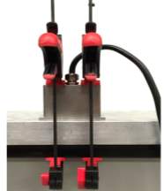
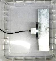
| Figure 3: (a) Direct contact experiment setup where the transducer and specimen were clamped (b) Immersion experiment setup with a spacer (circled in red) between the transducer and specimen………………………………………………………………….. | 9 |
| Figure 4: Graph of amplitude vs time for all 64 pulse echo signals.……………… | 100 |
| Figure 5: (a) Direct contact and (b) Immersion propagation distance of wave from one transmitter to another receiver …………………………………………………. | 10 |
| Figure 6: Model illustrating the angles for (a) direct contact and (b) immersion calculated using Snell’s Law (5eproduced from [8])…………………………………… | 11 |
| Figure 7: Amplitude vs time graph (a) before applying filter and (b) after applying filter….……………………………………………………..……………………. | 12 |
| Figure 8: Graph showing envelope of signal over original signal after Hilbert transform …………..………….…………………………………………………………… | 14 |
| Figure 9: Directivity function before averaging over similar longitudinal angle…. | 15 |
| Figure 10: 1D array transducer sectioned into
mparts resembling a 2D array transducer.…………………………………………………………………………………….. |
17 |
| Figure 11: Direct contact convergence test graphs using (a) Array 1 (5MHz, 0.6mm pitch) and (b) Array 3 (15MHz, 0.21mm pitch)…………………………………
|
18 |
| Figure 12: Immersion convergence test graphs using (a) Array 2 (5MHz, 0.6mm pitch) and (b) Array 3 (15MHz, 0.21mm pitch)…………………………………………
……………. |
18 |
| Figure 13: (a) Constant and (b) None constant value of loading shape over the width of array transducer element………………………………………………………..
|
|
| Figure 14: Parameters of geometry showing the far field response (Reproduced from [3]).………………………………………………………………………………………. | 19 |
| Figure 15: Graph of numerical and analytical theoretical directivity function vs angle.……………………………………………………………………………………….. | 20 |
| Figure 16: Loading shapes of signal from the transmitting element of width 0.185mm at different values of
wfor (a) Gaussian curve and (b) Sinc curve…………… |
20 |
| Figure 17: Direct contact directivity function graph of Array 1 (5MHz, 0.6mm pitch) for specimen with 1.5cm thickness. The value of
w=10and m=20…………. |
21 |
| Figure 18: Direct contact directivity function graph of Array 1 (5MHz, 0.6mm pitch) for specimen with 2cm thickness. The value of
w=10and m=20…………… |
21 |
| Figure 19: Direct contact directivity function graph of Array 3 (15MHz, 0.21mm pitch) for specimen with 1.2cm thickness. The value of
w=26and m=11…………. |
22 |
| Figure 20: Direct contact directivity function graph of Array 3 (15MHz, 0.21mm pitch) for specimen with 1.5cm thickness. The value of
w=26and m=11…………. |
22 |
| Figure 21: Direct contact directivity function graph of Array 3 (15MHz, 0.21mm pitch) for specimen with 2cm thickness. The value of
w=26and m=11…………… |
23 |
| Figure 22: Immersion directivity function graph for (a) short solid specimen and (b) sampling bit…………………………………………………………………………………………………… | 23 |
| Figure 23: Immersion directivity function graph of Array 2 (5MHz, 0.63mm pitch) for distance 0.8cm between specimen and array. The value of
w=0.3and m=100… |
24 |
| Figure 24: Immersion directivity function graph of Array 2 (5MHz, 0.63mm pitch) for distance 1.5cm between specimen and array. The value of
w=1.5and m=100… |
24 |
| Figure 25: Immersion directivity function graph of Array 3 (15MHz, 0.21mm pitch) for distance 0.8cm between specimen and array. The value of
w=1.5and m=80….. |
25 |
| Figure 26: Immersion directivity function graph of Array 3 (15MHz, 0.21mm pitch) for distance 1.5cm between specimen and array. The value of
w=1.5and m=80….. |
25 |
| Figure 27: Amplitude vs time plot for all 64 receiving elements from transmitter element 1. The black circle represents the useful signals used to calculate directivity function while the blue circle shows the interference of useful signal by unknown signals | 28 |
List of Tables
| Table 1: Details of the phased array transducers used in the project…………… | 7 |
| Table 2: Wave propagation speed and density of aluminium and water……….. | 11 |
| Table 3: Correlation values of experimental and theoretical directivity functions for Array 1 (5MHz, 0.6mm pitch). Values in bold are the highest correlation coefficient.…………………………………………………………………………………. | 22 |
| Table 4: Correlation values of experimental and theoretical directivity functions for Array 3 (15MHz, 0.21mm pitch). Values in bold are the highest correlation coefficient….………………………………………………………………………………. | 23 |
| Table 5: Correlation values of experimental and theoretical directivity functions for Array 2 (5MHz, 0.63mm pitch). Values in bold are the highest correlation coefficient.….……………………………………………………………………………… | 24 |
| Table 6: Correlation values of experimental and theoretical directivity functions for Array 3 (15MHz, 0.21mm pitch). Values in bold are the highest correlation coefficient….………………………………………………………………………………. | 25 |
| Table 7: Details of the arrays used for the experiments..………………………… | 26 |
1. Introduction
Ultrasound is used to perform non-destructive evaluation (NDE) for investigating materials and structures[3]. Unlike other tests, NDE investigates the specimen without destroying it and therefore allowing it to be usable after the test[4]. This method is fast, simple, reliable and inexpensive. However, ultrasonic methods are indirect methods[3]. During the NDE test, the transmitted and then received acoustic wave is recorded in the form of electric voltage amplitude against time signals. These signals have no direct correlation with the properties of materials and signal processing must be done to extract quantitative information and investigate on the properties and defects present in the materials.
Ultrasonic testing can be done using both single element transducer and phased array transducer. In this project, phased array transducer was used as it provides a greater flexibility by allowing the user to obtain a range of different inspections[5] from a single location. A phased array consists of an array of piezoelectric elements. Each element can be driven separately by sending a pulse of signal to the specimen and the reflected signal is received by all array elements independently[3]. Ultrasonic phased array transducer can be classified as one-dimension (1D) and two-dimension (2D) array but this project focused on the use of 1D phased array transducer.
The aim of this project is to investigate on the ultrasonic phased array element directivity function. Directivity function is utilised to define the angular distribution of the transmitted ultrasonic field of each array transducer element[5]. The project focuses mainly on validating the 1D theoretical directivity functions obtained analytically and numerically with experimental directivity function measured using direct contact and immersion techniques. If the model is validated, theoretical directivity function can be used to predict the characteristics of defects present in a specimen as well as determine the lifetime and usability of a specimen with defects.
2. Experimental Method
2.1 Phased Array Transducer
In this project, 1D array transducers with equal spacing between the
nnumber of elements were used (see Figure 1). The wave transmitted by each element was assumed to move only in the x-z plane only. The length of element in y direction was assumed to be infinitely long which allowed the transducer to be modelled as a 2D problem. Three types of 1D array provided by Immasonic were used in this project and the details are summarised below:
| Array | Serial Number | Centre Frequency,
f (MHz) |
Number of elements,
n |
Element Pitch,
p (mm) |
Element Width,
a (mm) |
Element Length,
l (mm) |
| 1 | 12208 1001 | 5 | 64 | 0.60 | 0.50 | 10 |
| 2 | 4154 A101 | 5 | 64 | 0.63 | 0.53 | 15 |
| 3 | 6485 A101 | 15 | 64 | 0.21 | 0.185 | 5 |
Table 1: Details of the phased array transducers used in the project.
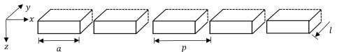
Figure 1: Geometry of a phased 1D array transducer (Reproduced from [1])
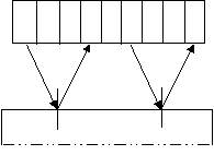
2.2 Full Matrix Capture
Full Matrix Capture (FMC) is a data acquisition process that uses the phased array transducers[6]. For a 1D array transducer with
nnumber of elements, the elements can behave as transmitter,
txand receiver,
rx. During FMC, each element will take turns to act as a transmitter, while all the
nelements will behave as receivers. All the signals captured will be stored as a
n × nmatrix. If the same element is used as both transmitter and receiver, the signal collected is known as pulse echo signal. The pulse echo term will be used frequently in the rest of the sections. During the experiments, FMC was used to collect the useful data.
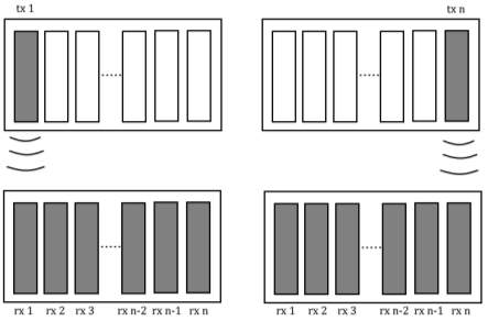
Figure 2: Illustration of full matrix capture (Reproduced from [2])
2.3 Experimental Setup
Experiments to investigate the directivity function in both direct contact and immersion were conducted. The experimental setup consisted of three main components: array transducer, MicroPulse FMC and BRAIN software. The array transducer was connected to the MicroPulse FMC which is an ultrasonic wave inspection platform (equivalent to a pulse-receiver device). The MicroPulse FMC was connected to the PC via an Ethernet cable and the ultrasonic array data acquired could be viewed using BRAIN software. For this project, the aluminium specimen was used throughout the entire project.
2.2.1 Direct Contact
During the experiment, the coupling gel was applied between the array transducer and the aluminium specimen. The coupling gel allowed the longitudinal wave to be transferred efficiently from the transducer to the specimen with minimum loss of energy due to attenuation and absorption [7]. To ensure a constant coupling throughout the surface when running the scan with MicroPulse FMC, the specimen and transducers were clamped together (see Figure 3(a)).
On the BRAIN software, the FMC setting was chosen. The averaging setting was set to 10 rather than 1. This means that 10 sets of readings were obtained and the mean amplitude was stored as the data captured. The averaging method allowed signal to noise ratio to be improved [1] and the amplitude signal to be smoothen. The amplitude of transmitter 1 to receiver 1 pulse echo signal was examined using Matlab. If an extremely high gain was set on BRAIN when collecting the data, it could be observed that the signal amplitude would exceed the allowable range thus causing the signal to be chipped. The gain setting was adjusted accordingly until the amplitude data was not chipped away to ensure no loss of data.
The experiment was repeated with the same settings on BRAIN at different positions of the same specimen and the data captured was saved. The data of the same specimen thickness would be averaged during post processing to reduce noise and ensure a smoother curve.


clamp
specimen
array
array
water tank
spacer
specimen
(a)
(b)
Figure 3: (a) Direct contact experiment setup where the transducer and specimen were clamped (b) Immersion experiment setup with a spacer (circled in red) between the transducer and specimen
2.2.2 Immersion
During the experiment, water was used as coupling agent between the array transducer and aluminium specimen. Immersion testing has a better advantage over direct contact testing as the water bath provides a constant coupling between the transducer and specimen[7].
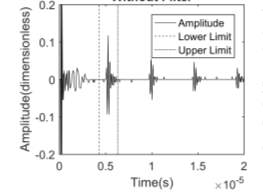
One of the key challenges when conducting the immersion testing was to ensure that the array transducer was parallel to the solid specimen. Two methods were enforced to ensure both parts were parallel. Method one involves pushing a spacer between the specimen and transducer. Then, the spacer was removed with care (see Figure 3(b) circled in red) leaving a gap with fixed separation between the array transducer and specimen. The second method was to use Matlab to examine the amplitude signals recorded. To detect whether both parts are parallel, the time of arrival for all
nnumbers of pulse-echo signals were examined. If parallel, the time of arrival for all pulse-echo signals would be approximately constant as the distance between the parts were constant. A window with a fix lower and upper limits from the estimated time of arrival was set (see Figure 4). If the overall signal dropped outside of the upper or lower limit, the array transducer is not parallel to the specimen and the Matlab code would not proceed with the post-processing.
During experiment, FMC was configured on the BRAIN software. The averaging setting was set to 64 rather than 1. This means that 64 sets of readings were obtained and the mean amplitude was stored as the data captured. The averaging setting was 10 for direct contact rather than 64. In previous testing, if 64 was chosen, the mean results obtained were less accurate. The standard deviation in data collected was greater in direct contact if the averaging is too long because it is harder to maintain the same experimental condition throughout one scan. After trial and error with different averaging values, average 10 was chosen as it yielded an optimum result.
The gain of amplitude was adjusted using the similar method to the direct contact testing until no amplitude data was chipped away. The experiment was repeated at different positions with the same settings on BRAIN, array transducer, specimen and separation distance between both parts for more averaging during post processing.
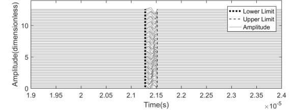
Figure 4: Graph of amplitude vs for all 64 pulse echo signals.
3. Measurement of Experimental Directivity Function
The overall numerical method model to obtain experimental directivity function for both direct contact and immersion were the same. The major difference would be the formula used to calculate the reflection coefficient in Section 3.6.
3.1 Calculation of Propagation Distance
(a)
(b)
Figure 5: (a) Direct contact and (b) immersion propagation distance of wave from one transmitter to another receiver
The transmit-receive signal combination was assumed to be a reflection symmetry at the mirror line at position
xmid(see Figure 5). Therefore, the propagation distance
dtxfrom the transmitter to the specimen wall is similar to the propagation distance
drxfrom the specimen wall to the receiver. The total distance
dtx,rxcan be calculated using the Equation 1 below
| dtx,rx= 2xc- xmid2+z2 | ( 1 ) |
where
xcis the position of the transmitting array,
xmidis the mid-point between the centre of transmitting and receiving array and
zis the specimen thickness for direct contact and the distance between transducer array and specimen for immersion.
3.2 Wave Propagation Speed and Density
According to Schmer[7], the wave propagation speed and density are summarised in Table 2. For accuracy, the wave speed for aluminium and water used in the post-processing would be calculated from the experimental data collected instead. The wave speed by Schmer would only be used as a reference point to ensure the validity of wave speed estimated from the experiment.
To calculate the longitudinal wave speed
VL, the time of arrival for the reflected pulse echo wave had to be estimated first. From the amplitude scan (A-scan) of a pulse echo signal, the starting point of the reflected signal from the wall of specimen was treated as the time of arrival of the signal,
ttx,rx. The longitudinal wave speed can be calculated with
| VL=dtx,rxttx,rx | ( 2 ) |
where
dtx,rxis the specimen thickness for direct contact and distance between array and specimen for immersion. As the experimental data was collected using a longitudinal wave array transducer, the shear wave speed in aluminium cannot be calculated directly from the A-scan data. According to Drinkwater[5], the shear wave speed in aluminium can be approximated as two times slower than the longitudinal wave speed. The values in bold calculated in Table 2 were used for the post-processing in the sections below.
| Material | Longitudinal Wave Speed,
VL(ms-1) |
Shear Wave Speed,
Vs (ms-1) |
Estimated Longitudinal Wave Speed,
VL (ms-1) |
Estimated Shear Wave Speed,
Vs (ms-1) |
Density,
ρ(kgm-3) |
| Aluminium | 6420 | 3040 | 6172 | 3086 | 2700 |
| Water | 1480 | – | 1427 | – | 1000 |
Table 2: Wave propagation speed and density of aluminium and water.
3.3 Calculation of Longitudinal and Shear Wave Angles
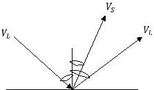
(b)
(a)
Figure 6: Model illustrating the angles for (a) direct contact and (b) immersion calculated using Snell’s Law (Reproduced from [8])
As the reflection is symmetry, the incident longitudinal angle
θLis equal to the received longitudinal angle for both direct contact and immersion.
In solid, there are two types of waves: longitudinal wave and shear wave whereas liquid has only longitudinal wave. The incident longitudinal wave angle for direct contact and immersion were calculated using
| tan-1θL=xc- xmidZ | ( 3 ) |
3.3.1 Direct Contact
The shear angle
θSin Figure 6(a) was calculated using Snell’s law [7]
| sinθSVs= sinθLVL | ( 4 ) |
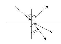
3.3.2 Immersion
By using Snell’s Law [7] below, the angle
θL2and
θS2transmitted into solid shown in Figure 6(b) were calculated using
| sinθL1VL1= sinθS2Vs2= sinθL2VL2 | ( 5 ) |
3.4 Calculation of Time of Arrival
The estimated time of arrival
ttx,rx’for each transmit-receive combination was calculated using Equation 2. With the estimated time of arrival, the actual time of arrival could be calculated. By referring to the A-scan of each transmit-receive combination, a time window of
ttx,rx’± ∆twas set. From the time window, the actual time of arrival
ttx,rxfor the signal could be chosen based on the time when the maximum amplitude signal was received.
3.5 Removal of Unwanted Signals
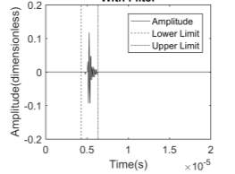
 With the actual time of arrival, a time window with a lower and upper limit could be applied to each transmit-receive combination amplitude recorded (see Figure 7). Those signals outside of the lower and upper limits were re-assigned with amplitude of value zero to filter away unwanted signals and noise. The choice of lower and upper limit values is important as it affects the experimental directivity function tremendously.
(b)
(a)
Figure 7: Graph of amplitude vs time (a) before applying filter and (b) after applying filter.
3.6 Calculation of Reflection Coefficient
Reflection coefficient was applied to calculate the intensity of signal amplitude reflected from the wall of specimen. The reflection coefficient for direct contact was calculated with [8]
| RDCθ= sin2θssin2θL-(VLVS)2cos22θSsin2θssin2θL+(VLVS)2cos22θS | ( 6 ) |
While, the equation for reflection coefficient for immersion is [8]
| RIMMθ= ρ2VL2cosθL2cos22θS2+ ρ2VS2cosθS2sin22θS2- ρ1VL1cosθL1ρ2VL2cosθL2cos22θS2+ ρ2VS2cosθS2sin22θS2+ ρ1VL1cosθL1 | ( 7 ) |
where
ρ1is the density of water and
ρ2is the density of aluminium that could be obtained from Table 2.
3.7 Amplitude Extraction Method
3.7.1 Type 1: Frequency Domain Signal – Fast Fourier Transform
During the signal processing, fast Fourier transform (FFT) was performed. FFT is an efficient algorithm which can compute discrete Fourier transform (DFT). DFT is a discrete version of Fourier transform which converts discrete time domain signal to discrete frequency domain signal. Let
x[t]be determined between the range
0<t<Tand sample the frequency at locations
fkwhere
kis the index of the sample [9]. The spectrum of the discrete time signal can be obtained with the formula below
| XD[fk]=∑t=0Tx[t]e-i2πtfk | ( 8 ) |
The filtered time domain signal obtained from Section 3.5 would be used as an input to FFT in the project. Absolute spectrum of FFT at frequency closest to the centre frequency of array transducer used was chosen to compute experimental directivity function. Extracting the signal in the frequency domain allowed only the useful signal to be sampled and therefore increasing the accuracy of post-processing.
3.7.2 Type 2: Time Domain Signal – Hilbert Transform
Hilbert transform could be used to obtain the discrete time analytic signal from the amplitude received to form the envelope of the amplitude signal (see Figure 8). Below are the steps to conduct Hilbert transform[10] to extract the useful amplitude signal:
- Calculate FFT of the input signal (filtered amplitude signal) and store it as vector H
- Set zero to components of H with negative frequencies and create vector Z(m) where
| Zm= 1 for m=1, (n2+1)2 for m=2,3,…, n20 for m= n2+2 ,…, n | ( 9 ) |
- Obtain the product of both vectors H and Z
- Calculate the inverse of FFT using the output from Step III.
- Obtain the absolute of inverse FFT and use it to plot the envelope
- Extract the maximum amplitude of signal from the new signal envelope for each transmit-receive combination to calculate the experimental directivity function.
 To achieve one-sided spectrum, in step II the negative frequency components were neglected due to the Hermitian symmetry with no loss of information.
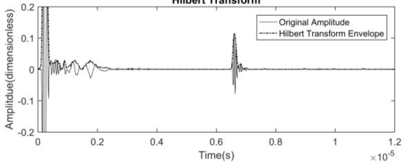
Figure 8: Graph showing envelope of signal over original signal after Hilbert transform.
3.8 Calculation of Normalised Experimental Directivity function
The amplitude of reflected signal,
uθLfor 1D array transducer is expressed using the relationship
| uθL= uoωRθD2(ω,θL)dtx,rx | ( 10 ) |
where
uoωis assumed to be the initial pulse for frequency domain signals,
Rθis the reflection coefficient and
D2ω,θLis the single element directivity function.
D2ω,θLis the product of directivity in the transmit mode and directivity in the receive mode. Rearranging Equation 10, the experimental directivity function
D2(ω,θL)for all
n2transmit receive combination can be calculated in terms of
uoω.
| D2(ω,θL)=uθLdtx,rxRθ(1uoω) | ( 11 ) |
The experimental directivity functions of the similar longitudinal angle
θLwere sorted together (see Figure 9) and the mean value for each longitudinal angle was obtained. Averaging over similar angles was done to minimise the effect of element differences as each element was assumed to perform slightly different from one another due to manufacturing limitation.
As the term
uoωis unknown but constant for all
θL, it can be factorised away by normalising
uθLto
u0for all angles of
θL. Rearranging Equation 11, the normalised experimental directivity can be expressed as
| D(ω,θL)D(ω,0)= ucompθLucomp0 | ( 12 ) |
where
| ucompθL=uθLdtx,rxRθ | ( 13 ) |
and
uθLis either the amplitude in the frequency domain obtained after FFT or amplitude in time domain obtained after Hilbert transform.
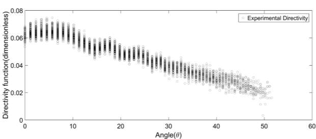
Figure 9: Graph of directivity function before averaging over similar longitudinal angle.
4. Calculation of Theoretical Directivity Function
4.1 Analytical Theoretical Directivity Function
In Huygens Principle, the wave aperture can be described as the summation of a row of infinitesimally small point sources for a 3D model or line sources for a 2D model [11]. The summation of sources allows the array element surface to be modelled.
According to Schmer[3], if the specimen thickness for direct contact or the distance between array transducer and specimen for immersion is greater than three times the near field length
H, the wave field of an array element can be modelled as far field. Near field length
His expressed as
| H=b2λ | ( 14 ) |
where
bis half of the element width,
a, and
λis the ultrasound wavelength. By satisfying the far field condition, the closed form solutions known for the field from simple element shapes could be used to calculate the far field directivity function[5]. The directivity function of finite element size,
Dfis
| Dfω,θL=sinc(πasinθLcosϕλ(ω))sinc(πLsinθLsinϕλ(ω)) | ( 15 ) |
where
ais the width and
Lis the length of transducer element,
θLis the longitudinal angle and
ϕis the azimuth angle. For a 1D array, each element was assumed to be an infinitely long strip source in the y direction. When the element length is much greater than the element width, it could be treated as a 2D problem[12]. By setting
ϕ=0, directivity function of element in 2D plane can be expressed as
| Dfω,θL=sinc(πasinθLcosϕλ(ω)) | ( 16 ) |
The directivity of longitudinal wave due to line loading on the surface of a semi-infinite elastic solid in 2D case is given as
| DLθL= VLVs2-2sin2θLcosθLF0(sinθL) | ( 17 ) |
where
VLis the bulk longitudinal velocity,
VSis the bulk shear velocity and
| F0ζ= 2ζ2-(VLVS)22-4ζ2(ζ2-1)1/2ζ2-(VLVS)21/2 | ( 18 ) |
In direct contact, the far field 1D directivity function,
Ddwas calculated using the relationship
| Ddω,θL= Dfω,θLDLθL | ( 19 ) |
In immersion, the far field 1D directivity function,
Diis
| Diω, θL= Dfω,θL | ( 20 ) |
The directivity function in Equation 18 and 19 are valid only for the far field region and not the near field region. Far field directivity functions for both direct contact and immersion were normalised by far field directivity at angle
θL=0so that the maximum normalised directivity function would be the value 1. This eases the comparison between graphs in Section 5.
4.2 Numerical Theoretical Directivity Function
4.2.1 Finite Element Length
The analytical 1D directivity function in Section 4.1 was derived based on the assumption such that each element of the array behaves like an infinite length strip source in the y-direction[5]. This is not always the case especially when small array transducer has a shorter element length
l. This section will discuss on how the theoretical directivity function with finite length of elements was derived.
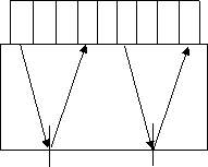
Assuming each element of the transducer is sectioned into
mparts in the y-direction as shown in the Figure 10 below, it resembles a 2D array transducer instead. Each element of array transducer would be subdivided into length
lm. The azimuth angle
ϕshown in Figure 10 could be calculated using
| tan-1ϕ=y’x’ | ( 21 ) |
where
x’is the distance between the mid-point of two array elements in the x-axis and
y’is the distance between the mid-point of two subdivided sections of the same array element in the y-axis.
Since the geometry of array transducer is known and the elements now have finite element length
lm, the theoretical directivity function of finite size element
D(ω,θL) could be calculated.
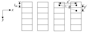
Figure 10: 1D array transducer sectioned into
mparts resembling a 2D array transducer.
Firstly, the analytical 2D theoretical directivity function for direct contact
Dd(ω,θL,ϕ)and immersion
Di(ω,θL,ϕ)could be expressed as
| Dd(ω,θL,ϕ)=Dfω,θL,ϕDLθL | ( 22 ) |
and
| Diω, θL,ϕ= Dfω,θL,ϕ | ( 23 ) |
where
Dfω,θL,ϕbelongs to Equation 14 and
DLθLbelongs to Equation 16. By slightly altering the amplitude of reflected signal relationship from Equation 10 to
| um*θL= uoωRθD2(ω,θL,ϕ)dtx,rxeikdtx,rx | ( 24 ) |
for 2D array, the amplitude received by each subdivided part
um*θLcould be calculated using the analytical theoretical 2D directivity function
Dd(ω,θL,ϕ)or
Diω, θL,ϕas
Dω, θL,ϕand
RDCθor
RIMMθas
Rθ. In Equation 23, the phase delay term
eikdtx,rx where
k(the wave number) is
2πλwas introduced. Phase delay term was added to account for the phase difference present in the subdivided transmitter-receiver parts of each array element. Since 2D array assumes each element as a point source rather than line source, the denominator of Equation 23 would be
dtx,rxrather than
dtx,rx.
The amplitude of signals found were summed up together for receivers which belongs to the same element using
| uθL=∑1mum*θL | ( 25 ) |
The
uθLfound in Equation 24 was substituted back to Equation 12 and 13 to calculate the finite length theoretical directivity function.
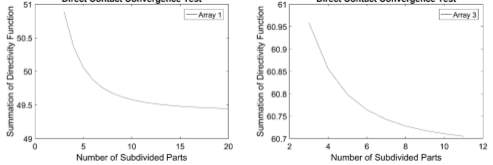
A convergence study was conducted to determine the suitable value of
mfor each array transducer in direct contact and immersion. Iteration with progressively increasing values of
mstarting with value 2 was conducted until the summation of finite length directivity function converges. Due to computational limits, the maximum number of
mwas set at 100. The iteration stopped when the absolute difference in percentage between summation of directivity functions at
mand
m-1is less than 0.01%.
According to Figure 11, it can be observed that Array 1 converges at
m=20and Array 3 converges at
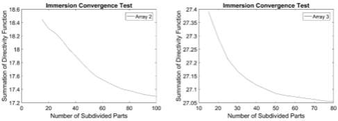
m=11. Based on Figure 12(a), Array 2 reaches
m=100. Nevertheless, the absolute difference in percentage between summation of directivity functions at
mand
m-1is 0.1%, which is still accurate. While, for Array 3 it converges at
m=80.The
mvalues computed would be used to calculate the finite length directivity in the results sections.

(a)
(b)
Figure 11: Direct contact convergence test graphs using (a) Array 1 (5MHz, 0.6mm pitch) and (b) Array 3 (15MHz, 0.21mm pitch).

(a)
(b)
Figure 12: Immersion convergence test graphs using (a) Array 2 (5MHz, 0.63mm pitch) and (b) Array 3 (15MHz, 0.21mm pitch)
4.2.1 Varying Signal Shape
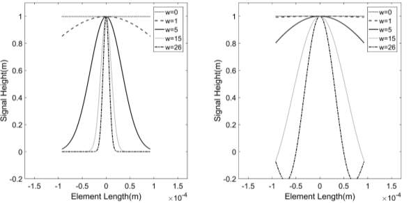
The analytical theoretical directivity function in Section 4.1 assumed the signal in the far field has a constant value of loading shape over the width of element (see Figure 13(a)). This section focuses on deriving and investigating the effects of directivity functions that have other shape functions such as Gaussian and Sinc shape (see Figure 13(b)).


(b)
(a)
Figure 13: (a) Constant and (b) None constant value of loading shape over the width of array transducer element.
According to Figure 1, the element of array transducer with width
acould be divided into infinitely small parts, each representing a line source. The amplitude of line source,
ul, is described using the relationship
| ul=A(x)P(θL)reikr | ( 26 ) |
where
A(x)is the shape function,
P(θL)is either 1 for immersion or the directivity of line source
DLθLfrom Equation 16 for direct contact and
ris the distance between points. Using the laws of cosine, distance
rshown in Figure 14 can be expressed as[3]
| r= ro2+x2-2xrosinθL | ( 27 ) |
Assuming
xo,zshown in Figure 14 is in the far field, it can be stated that
xro≪1. Equation 26 can then be expanded to first order [3] as
| r≈ ro-xsinθL | ( 28 ) |
Also,
| 1r≈1ro | ( 29 ) |
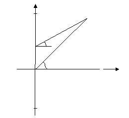
Figure 14: Parameters of geometry showing the far field response(Reproduced from [3]).
Substituting Equation 27 and 28 to Equation 25 and integrating it over the range of
xfrom
-a2to
a2to sum up the amplitude from all line source of an element, the equation can be expressed as
| u≈P(θL)ro∫-a2a2A(x)eik(ro-xsinθL) dx | ( 30 ) |
Rearranging Equation 29, it can be expressed as
| u≈eikroroD(ω,θL) | ( 31 ) |
where the numerical theoretical directivity function
Dω,θLcan be expressed as
| Dω,θL=P(θL) ∫-a2a2A(x)e-ikxsinθL dx | ( 32 ) |
The directivity function integral in Equation 31 can be solved for all
θLto obtain the numerical theoretical directivity function.
First, to verify the method, the numerical theoretical directivity function with constant value of loading shape over the width of element would be derived to compare with the analytical theoretical directivity function from Section 4.1. To calculate the directivity function with constant value of loading shape over the width of the element,
A(x)was substituted as 1. The graph of analytical theoretical directivity from Section 4.1 was plotted against the numerical theoretical directivity and shown in Figure 15 below.
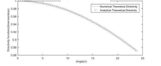
Figure 15: Graph of numerical and analytical theoretical directivity function vs angle.
Based on Figure 15, it can be observed that the plots are identical with one another. Thus, the method is valid. To consider other shape functions,
A(x)can be substituted with different expressions. To express the Gaussian loading shape,
A(x)can be expressed as
| A(x)= 12σ2πe-(wxλ-μ)22σ2 | ( 33 ) |
where
σis the standard deviation of the shape,
wis the scaling factor and
μis the mean. The value of
σand
μused throughout the project would be remained constant.
σ=0.4would be used to ensure the maximum signal height is 1 (see Figure16(a)). While,
μ=0would be used to ensure the curve is symmetric along y-axis. To express the Sinc loading shape,
A(x)can be described as
| A(x)=sinc(wxλ) | ( 34 ) |
By varying the value of
win Equation 32 and 33, the sizes of Gaussian and Sinc loading shapes can be varied (see Figure 16).
(a)
(b)
Figure 16: Loading shapes of signal from the transmitting element of width 0.185mm at different values of
wfor (a) Gaussian curve and (b) Sinc curve.
5. Results
5.1 Direct Contact
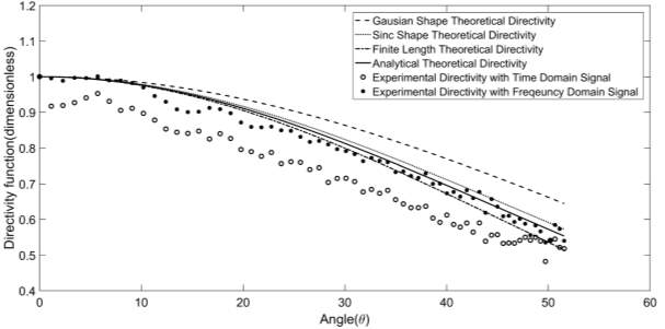
Figure 17: Direct contact directivity function graph of Array 1 (5MHz, 0.6mm pitch) for specimen with 1.5cm thickness. The value of
w=10and
m=20.
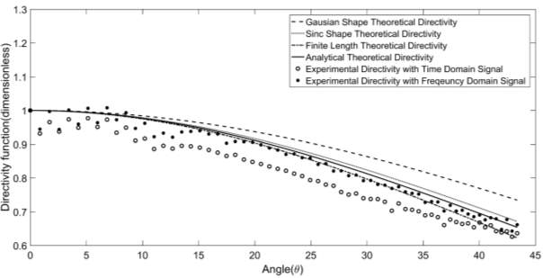
Figure 18: Direct contact directivity function graph of Array 1 (5MHz, 0.6mm pitch) for specimen with 2cm thickness. The value of
w=10and
m=20.
| Specimen Thickness(cm) | Gaussian | Sinc | Finite Length | Analytical | |
| Frequency Domain | 1.5 | 0.991984 | 0.993405 | 0.993434 | 0.993594 |
| Time Domain | 0.976809 | 0.981806 | 0.981902 | 0.982795 | |
| Frequency Domain | 2.0 | 0.991036 | 0.991735 | 0.991772 | 0.991817 |
| Time Domain | 0.982160 | 0.985433 | 0.985724 | 0.986078 |
Table 3: Correlation values of experimental and theoretical directivity functions for Array 1 (5MHz, 0.6mm pitch). Values in bold are the highest correlation coefficient.
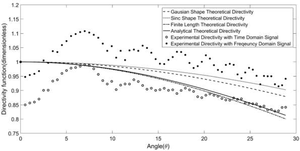
Figure 19: Direct contact directivity function graph of Array 3 (15MHz, 0.21mm pitch) for specimen with 1.2cm thickness. The value of
w=26and
m=11.
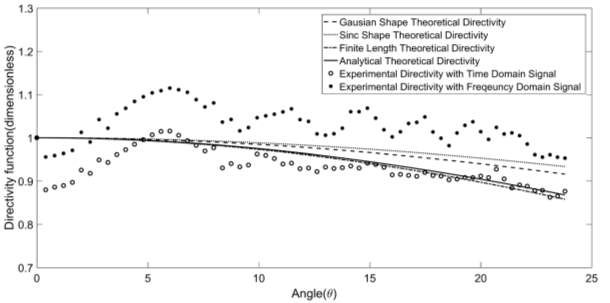
Figure 20: Direct contact directivity function graph of Array 3 (15MHz, 0.21mm pitch) for specimen with 1.5cm thickness. The value of
w=26and
m=11.
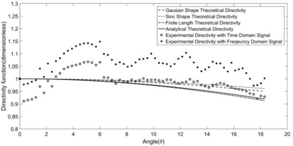
Figure 21: Direct contact directivity function graph of Array 3 (15MHz, 0.21mm pitch) for specimen with 2cm thickness. The value of
w=26and
m=11.
| Specimen Thickness(cm) | Gaussian | Sinc | Finite Length | Analytical | |
| Frequency Domain | 1.2 | 0.710746 | 0.713258 | 0.707522 | 0.707255 |
| Time Domain | 0.766884 | 0.767606 | 0.765822 | 0.765729 | |
| Frequency Domain | 1.5 | 0.495133 | 0.498097 | 0.491502 | 0.491318 |
| Time Domain | 0.680698 | 0.681806 | 0.679280 | 0.679207 | |
| Frequency Domain | 2.0 | 0.408283 | 0.410682 | 0.405405 | 0.405331 |
| Time Domain | 0.483062 | 0.484690 | 0.481099 | 0.481048 |
Table 4: Correlation values of experimental and theoretical directivity functions for Array 3 (15MHz, 0.21mm pitch). Values in bold are the highest correlation coefficient.
5.2 Immersion
(a)
(b)
Figure 22: Immersion directivity function graph for (a) short solid specimen and (b) sampling bit 8.
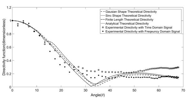
Figure 23: Immersion directivity function graph of Array 2 (5MHz, 0.63mm pitch) for distance 0.8cm between specimen and array. The value of
w=0.3and
m=100.
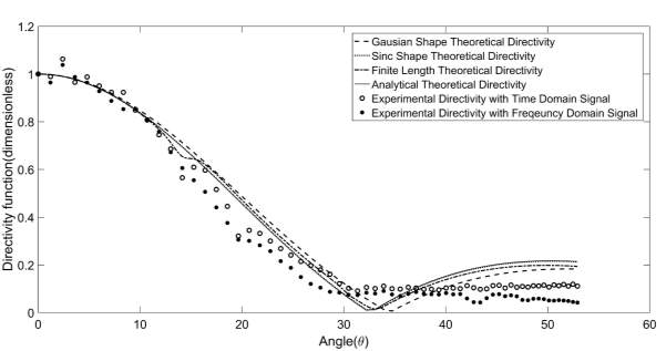
Figure 24: Immersion directivity function graph of Array 2 (5MHz, 0.63mm pitch) for distance 1.5cm between specimen and array. The value of
w=0.3and
m=100.
| Distance (cm) | Gaussian | Sinc | Finite Length | Analytical | |
| Frequency Domain | 0.8 | 0.974288 | 0.972292 | 0.970535 | 0.971967 |
| Time Domain | 0.975047 | 0.971330 | 0.969343 | 0.970885 | |
| Frequency Domain | 1.5 | 0.979573 | 0.977604 | 0.980190 | 0.977316 |
| Time Domain | 0.985195 | 0.982090 | 0.985701 | 0.981711 |
Table 5: Correlation values of experimental and theoretical directivity functions for Array 2 (5MHz, 0.63mm pitch). Values in bold are the highest correlation coefficient.
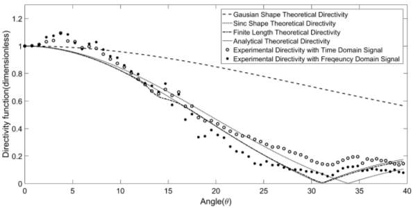 Figure 25: Immersion directivity function graph of Array 3 (15MHz, 0.21mm pitch) for distance 0.8cm between specimen and array. The value of
w=1.5and
m=80.
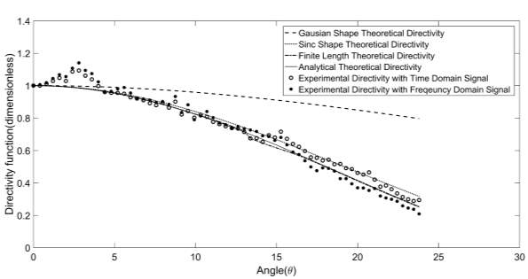
Figure 26: Immersion directivity function graph of Array 3 (15MHz, 0.21mm pitch) for distance 1.5cm between specimen and array. The value of
w=1.5and
m=80.
| Distance (cm) | Gaussian | Sinc | Finite Length | Analytical | |
| Frequency Domain | 0.8 | 0.914069 | 0.975770 | 0.987119 | 0.987124 |
| Time Domain | 0.939598 | 0.987385 | 0.991629 | 0.990001 | |
| Frequency Domain | 1.5 | 0.991523 | 0.993328 | 0.992234 | 0.993366 |
| Time Domain | 0.989216 | 0.991516 | 0.991148 | 0.991598 |
Table 6: Correlation values of experimental and theoretical directivity functions for Array 3 (15MHz, 0.21mm pitch). Values in bold are the highest correlation coefficient.
6. Discussion
The directivity functions against longitudinal angles
θlfor direct contact and immersion were plotted in Figure 17 to Figure 21 and Figure 22 to Figure 26. Both direct contact and immersion were conducted with 5MHz (Array 1 and 2) and 15MHz (Array 3) array transducers with different element sizes; big for 5MHz and small for 15MHz. The experimental directivity functions in frequency domain and time domain signals were plotted in circles while theoretical directivity functions were plotted in lines.
Due to normalisation, the experimental plot results might be shifted, depending on the value of experimental directivity function at longitudinal angle
θl=0. To ease the comparison process, Pearson’s product moment correlation coefficient was computed in Table 3 to 6 to investigate the similarity between the shape of curves[13]. The correlation coefficient values are a summary of the linear association between the experimental and theoretical directivity functions. Coefficient with the value closes to 1 indicates that both directivity functions are the most identical.
While computing the theoretical directivity functions, a few extra steps were taken to ensure an accurate analysis. For the Gaussian and Sinc theoretical directivity, iteration with progressively increasing values of
wbetween 0.1 to 30 was conducted.
wthat yielded the highest value of correlation coefficient for either Gaussian or Sinc shape directivity function with respect to frequency and time domain directivity functions would be chosen. If none of the
wvalues resulted in a better correlation with the experimental directivity functions than the finite length and analytical theoretical directivity, a random
wvalue would be chosen for the purpose of directivity function comparison.
Directivity function is independent of the specimen thickness for direct contact as well as distance between array and solid specimen for immersion. For each array, the experiment was conducted with at least two different thicknesses or distances to ascertain the directivity pattern.
The thicknesses or distances were chosen such that it is greater than the far field length 3H (see Section 4.1) calculated in Table 7 to ensure that the far field criterion when evaluating directivity function is fulfilled.
Based on the results in Section 5, the directivity function of direct contact and immersion follow the same pattern but it is steeper for immersion than direct contact due to the smaller wavelength of ultrasound in water. The ratio of element width
ato wavelength
λis shown in Table 7 below. As the ultrasound wave speed is approximately four times slower in water than aluminium, the wavelength is approximately four times smaller. Therefore, the ratio of element width to wavelength is greater in water. This results in a steeper directivity pattern in immersion than direct contact. Also, the spread of angle of directivity function is greater if the thickness or distance is smaller.
One of the assumptions made about the array transducer model when computing the experimental directivity function was that each strip source element acted in unison in a piston-like behaviour[3]. As each element strip source was assumed to be surrounded by rigid baffle, when one element fired the other elements were assumed to be totally isolated and have zero velocity. Unfortunately, this is not the case. According to Figure 17 to 26, at small angles it can be observed that there are oscillations in the experimental directivity pattern. According to Domínguez[14], when an element is excited, the vibration can be transmitted to the neighbouring passive elements and then exciting them if the mechanical isolation between the element are poor. This is known as cross-talk. One of the factors that affects the phenomenon is the element gap between array elements.
| Array 1 | Array 2 | Array 3 | ||
| Direct Contact | wavelength,
λd( mm) |
1.234 | – | 0.411 |
| Ratio of
ato λd |
0.4052 | – | 0.4501 | |
| Far field length,
3H ( mm) |
0.152 | – | 0.0625 | |
| Immersion | wavelength,
λi( mm) |
– | 0.285 | 0.0951 |
| Ratio of
ato λi |
– | 1.8596 | 1.9453 | |
| Far field length,
3H ( mm) |
0.739 | 0.270 | ||
Table 7: Details of the arrays (Array 1(5MHz, 0.6mm pitch), Array 2 (5MHz, 0.63mm pitch) and Array 3(15MHz, 0.21mm pitch)) used for the experiments.
According to Figure 19 to Figure 21 for direct contact and Figure 25 to Figure 26 for immersion, it can be seen that the experimental directivity pattern have very obvious oscillations even at large angles as compared to Figure 17 to Figure 18 and Figure 23 to Figure 24. As the 15MHz array has a much smaller element size and element gap compare to the 5MHz arrays, the effect of cross-talk is stronger. Comparing the experimental directivity function of 5MHz array to the 15MHz array in both direct contact and immersion, the oscillations in experimental directivity only present at small angles. At larger angles the distance required to be travelled by the transmitted signal to the receiver is longer. When the signal arrives at the respective element, the lateral vibration due to the excited element has been damped away. Therefore, the directivity functions at those angles for 5MHz arrays are more stable.
During generation of ultrasonic wave, the internal resonance of transducer element added a ringing effect to the transmitted pulse of signal. This caused an increase in the duration of transmitted pulse and decrease in signal resolution[15]. Ringing effect would affect the frequency domain signals because ringing effect could not be separated from A-Scan data. As experimental directivity for frequency domain signals were computed by extracting absolute spectrum value at the centre frequency, if the ringing effect has the same frequency, it will affect the accuracy of result. For this case, time domain signal might yield a more accurate result. This explains why some experiments have higher correlation values between theoretical and time domain experimental directivity than frequency domain experimental directivity.
6.1 Direct Contact
For Array 1 (5MHz, 0.63mm pitch), it can be observed that the coefficient values for analytical column in Table 3 are the highest for all specimen thicknesses in both frequency and time domain compare to other theoretical directivity functions. Iteration for
wfrom value 0.1 to 30 was conducted but none of the values yielded a coefficient value higher than the analytical and finite length theoretical directivity functions. A random
w=10 was chosen to compute the Gaussian and Sinc theoretical directivity for the purpose of directivity function comparison.
For Array 3 (15MHz, 0.21mm pitch), it can be observed that the coefficient values for Sinc column in Table 4 are the highest for all specimen thicknesses in both frequency and time domain compare to other theoretical directivity functions. The experiment was conducted with three different specimen thicknesses instead of two to ascertain the results. Iteration for
wwas conducted and
w=26was computed to have a correlation coefficient value higher than other theoretical directivity functions for all three different specimen thicknesses. In Table 4, Gaussian theoretical directivity yielded correlation values that are second closest to 1. In short, it can be proven that the assumption of having a loading shape with constant value over the width of element is inaccurate for this array and the emitted wave behaves more like a Sinc shape curve with
w=26(see Figure 16(b)).
6.2 Immersion
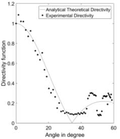
For immersion, in the initial stage there was an unexpected spike in the directivity pattern at 45 degree (see Figure 22(a)). The experiment was conducted with different distances between the array transducer and the solid specimen as well as different types of transducer. Unfortunately, the spike remained at approximately 45 degree. An investigation on the A-scan was conducted to identify the cause to the issue. The amplitude transmitted by element 1 to all
nelements were plotted in Figure 27 below. The black dotted line in Figure 27 shows the time of arrival of reflected signal from transmitter 1 to all receiving elements. According to Figure 27, the part circled in black represents the amplitude signal used to calculate experimental directivity function. The part circled in blue in the figure shows the interference of useful signal by some unknown signals. After conducting a thorough analysis, it was concluded that the unknown signals were the reflected wave due to the backwall of solid specimen and the shear wave in the solid specimen. To delay the time of arrival of other reflected waves, the experiment must be conducted using a solid specimen with a depth of length greater than the longest wave propagation distance
dtx,rxof all possible transmit receive combinations.
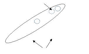
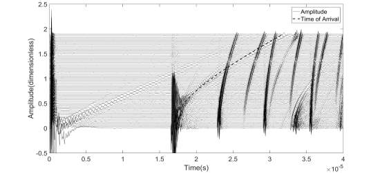
Figure 27: Amplitude vs time plot for all 64 receiving elements from transmitter element 1. The black circle represents the useful signals used to calculate directivity function while the blue circle shows the interference of useful signal by unknown signals.
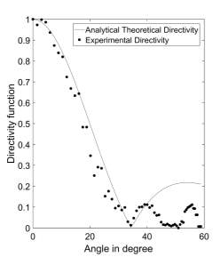
Moreover, for the early experiments it was conducted with the setting of sampling bit 8 on BRAIN software. Due to the low sampling bit, the resolution of amplitude captured is lower. From Figure 22(b), at the larger angles there was an unexpected drop in directivity function to zero value. Beam spread occurs because the ultrasound wave does not only travel in the direction of wave propagation. At large angles the required propagation distance of transmitted signal to receiver is longer, and therefore, the beam spreading is larger. The larger the beam spread, the greater the energy transferred to angles outside the direction of propagation. At some point, the amplitude was close to zero and due to lower sampling level, it was treated as a value of zero instead. To solve this problem, the sampling bit was increased to 16 so that the amplitude could be represented at more levels.
Iteration for
wfrom value 0.1 to 30 was conducted. If none of the values yielded a coefficient value higher than either the analytical or finite length theoretical directivity functions, a random value of
wwould be chosen. This value would be used to compute the Gaussian and Sinc theoretical directivity for the purpose of directivity function comparison in Figure 23 and 24 and the latter in Figure 25 and 26.
For Array 2 (5MHz, 0.63mm pitch), at a distance between array and solid specimen of 0.8 cm, Gaussian theoretical directivity yielded the highest correlation coefficient values for both time and frequency domain signals at w=0.3. While for distance between array and solid specimen of 1.5cm, the finite length theoretical directivity has the highest correlation coefficient values for all values of w. For the purpose of comparison, w=0.3 was chosen for distance 1.5cm. As mentioned before, directivity function is independent of the change in distance. The difference in result might be due to the experimental noise present. Nevertheless, the Gaussian and finite length theoretical directivity for both distances are nearly identical and both have values greater than 0.9 (strong correlation to experimental directivity). Therefore, the statement that directivity function is independent of the change in distance is still valid.
For Array 3 (15MHz, 0.21mm pitch), at distance of 0.8cm and 1.5cm most of the results yielded the highest correlation coefficient values with the analytical theoretical directivity function for all values of w. For the purpose of comparison, w=1.5 was chosen for both distances.
7. Conclusion and Future Work
All the experiments in direct contact and immersion yielded a close agreement to either type of the theoretical directivity functions. The theoretical directivity function can be used to estimate the reflection coefficient which then allows researchers to identify the properties of defects present in specimens in the future.
In general, immersion method is more reliable as it provides a better coupling between the array transducer and solid specimen. Also, the highest computed correlation coefficient values between experimental and theoretical directivity for each experiment were higher for immersion as compared to direct contact. As the correlation values are between 0.9 and 1, it can be concluded that experimental and theoretical directivity are strongly correlated.
For direct contact, the larger array tends towards the analytical theoretical directivity function. While for the smaller size array, the experimental directivity function showed a closer agreement to the Sinc theoretical directivity function. This proves that the assumption of having constant value of loading shape over the width of each array element is not valid for a smaller size array in direct contact.
Also, the assumption of array elements behaving as a piston-like model in computing the experimental directivity function is inaccurate. This is because a significant amount of oscillations could be observed in both direct contact and immersion experiments. A revised directivity model can be developed and tested in the future to factor in any cross-talk effect.
One interesting finding from this project is that the exact loading shape emitted by the excited array element does not always follow the line loading shape assumption in direct contact model. By using Equation 31 and varying the shape function for
A(x)and the value of
w, the actual loading shape can be predicted provided the experimental directivity function is known.
Due to the computational limitation, the number of subdivided parts of each transducer element,
m, of Array 2 (5MHz, 0.63mm pitch) in immersion could not be subdivided further smaller. The experiments can be repeated with a smaller element length until absolute tolerance between summation of finite length theoretical directivity function of
mand
m-1is less than 0.01% if a better computing device is available.
8. Reference
1. Holmes, C., B. Drinkwater, and P. Wilcox, Post-processing of the full matrix of ultrasonic transmit–receive array data for non-destructive evaluation in Department of Mechanical Engineering. 2005, University of Bristol. p. 701-711.
2. Zhou, Z., N. Xu, and F. He, Ultrasonic phased array inspection of L-shaped components based on dynamic aperture focusing. 2015: Beijing Hangkong Hangtian Daxue Xuebao.
3. Schmerr, L.W., Fundamentals of ultrasonic phased arrays. 1 ed. 2015: Springer International Publishing.
4. Introduction to Nondestructive Testing. Available from: https://www.asnt.org/MinorSiteSections/AboutASNT/Intro-to-NDT, accessed 6 March 2017.
5. Drinkwater, B. and P. Wilcox, Ultrasonic arrays for non-destructive evaluation: A review, in Department of Mechanical Engineering. 2006, University of Bristol. p. 526-540.
6. Full Matrix Capture. Available from: http://www.m2m-ndt.com/technology/FMC.htm, accessed 16 March 2017.
7. Schmerr, L.W., Fundamentals of ultrasonic nondestructive evaluation : a modeling approach. 1998, London ; New York: Plenum Press.
8. Cheeke, J.D.N., Fundamentals and applications of ultrasonic waves. CRC series in pure and applied physics. 2002, Boca Raton: CRC Press. 462 p.
9. II, R.J.M., The Joy of Fourier: Analysis, Sampling Theory, Systems, Multidimensions, Stochastic Processes, Random Variables, Signal Recovery, POCS, Time Scales, & Applications. 2006: Baylor University.
10. Marple Jr., S.L., Computing the Discrete-Time ‘Analytic’ Signal Via FFT Orincon Corporation. p. 1322-1325.
11. Shull, P., Nondestructive Evaluation-Theory, Techniques, and Applications. 2001: Marcel Dekker, Inc.
12. McNab, A. and I. Stumpf, Monolithic phased array for the transmission of ultrasound in NDT ultrasonics. 1985, University of Strathclyde.
13. LeBlanc, D.C., Statistics:Concepts and Applications for Science. 2004: Jones and Bartlett.
14. Domínguez, I., et al., Cross-talk Response Analysis on a Piezoelectric Ultrasonic Matrix Array. 2012.
15. Salim, M., et al., Study on ringing effect in ultrasonic transducer. 2012. p. 3682-3689.
Cite This Work
To export a reference to this article please select a referencing stye below:
Related Services
View all


Related Content
All TagsContent relating to: "Sciences"
Sciences covers multiple areas of science, including Biology, Chemistry, Physics, and many other disciplines.
Related Articles

DMCA / Removal Request
If you are the original writer of this dissertation and no longer wish to have your work published on the UKDiss.com website then please: