Deep Neural Networks for Prediction of Air Quality in Urban Environments
Info: 9174 words (37 pages) Dissertation
Published: 16th Dec 2019
Tagged: Environmental Studies
Deep Neural Networks for Prediction of Air Quality in Urban Environments
Abstract
Air pollution poses a major physiological threat to the public, especially those who reside in urbanised areas. It has been shown that early warning mechanisms enable vulnerable members of the public to be aware of potential future high pollution episodes, allowing them to modify their activities within the day or week to reduce their exposure to harmful air pollutants. Recent developments in air pollution forecasting applications include the utilisation of deep learning structures such as the Long Short-Term Memory (LSTM) neural networks. LSTM models were used in this study to extract inherent temporal features of historical air pollution time series. Hourly concentration levels of NO2, O3, PM2.5 and PM10, collected at the London Marylebone monitoring station in Central London from January to December 2015, were utilised to validate the proposed model. Twelve different models, i.e. one model for each air pollutant across three prediction horizons (12-, 24-, and 36-h ahead), were trained and compared using the same dataset. The experimental results exhibited that the LSTM model outperformed the benchmark ANN model, e.g. the Multilayer Perceptron (MLP), as indicated by several performance indices.
1. Introduction
Ambient air pollution is an environmental issue that continues to attract special legislative and scientific attention due to its adverse effects on public health and the economy [1]. Key air pollutants such as Nitrogen Oxides (NOx), particulate matter with an aerodynamic diameter of less than 10 µm (PM10) or 2.5 µm (PM2.5) and Ozone (O3) have been found to put strain on human cardiovascular and respiratory systems, thereby aggravating several illnesses [2]. According to the World Health Organisation (WHO), 4.2 million deaths per year were attributed to outdoor air pollution resulting in stroke, heart disease, lung cancer and chronic respiratory diseases [3]. Consequently, children, the elderly and those with pre-existing lung and heart conditions, and with lower incomes residing in highly urbanised areas were found to be most at risk [4]. Additionally, the health impacts of ambient air pollution were found to entail major economic consequences. For instance, the number of hospital cases directly associated with poor outdoor air pollution levels at a global level is projected to increase from 3.6 million in 2010 to 11 million in 2060, resulting in more health expenditures, restricted activity days and productivity losses [5].
Several legislative actions have been carried out to manage and minimise the emission levels of air pollutants at local and national scales. The European Union (EU) has set the Ambient Air Quality Directive (2008/50/EC) to provide threshold levels of ambient concentrations for key air pollutants to control the air quality amongst its member regions [6]. Additionally, the use of tools and schemes for peak air pollution prediction and smart traffic management can alleviate the effects of urban air pollution in various respects: 1) long-term forecasts enable legislators and urban city planners in making informed decisions to manage air pollution and traffic [7], and 2) short-term forecasts provide the public with early-warning updates that influence their daily behaviour during potential peak pollution events [8]. As such, several modelling approaches have been employed by the scientific and policy-making community in the past few decades.
Deterministic models attempt to characterise the generation, formation, and dispersion of air pollutants in the atmosphere via different equations [9]. Popular methods that have been employed in the past few decades include the Urban Airshed Model (UAM) [10], Weather Research and Forecasting Model with Chemistry (WRF/Chem) [11] and Community Multiscale Air Quality model (CMAQ) [12]. However, these models often require a large number of parameters, e.g. meteorological factors and topographical details of the immediate environment, making their implementation computationally expensive, time-consuming and difficult [13][14]. In addition, the random and complex mechanisms involved in air pollution modelling make it difficult to justify a deterministic approach for any reason other than reducing computation time, but this increases the risk of excessive oversimplification and reduced accuracy.
On the other hand, data-driven models apply various statistical techniques on a large amount of observations to reveal patterns instead of relying on sophisticated theoretical details. Several statistical forecasting approaches include Multiple Linear Regression (MLR) [15], Artificial Neural Networks (ANNs) [16], Support Vector Machine (SVM) [17], Fuzzy Logic (FL) [18] and hybrid models [19][20]. Among these models, ANNs have been used as forecasting tools in recent air pollution applications due to their overall superiority over traditional linear models [21]. ANNs can learn from patterns presented to them, and from the errors committed in their learning processes and can incorporate a large number of heterogeneous predictors at an impressive implementation speed [22]. Several forms of ANNs have been successfully developed and employed to improve the prediction of air pollution. Popular examples include the Multilayer Perceptron (MLP) [23], Radial Basis Function (RBF) network [14] and Neuro-Fuzzy (NF) network [24], with MLP being considered as the most widely used type [25][26]. However, models with simpler network architectures often encounter several difficulties: 1) characterisation of peak or rare values in a dataset [27], and 2) depiction of complex patterns within the massive datasets as open datasets grow more rapidly than ever [28].
Recent literature reveals the potential of incorporating deep or sophisticated neural network architectures in air pollution prediction [29]. Having multiple hidden layers has been examined and revealed to be capable of extracting high-level features from very large datasets without prior knowledge [30]. Qi et al. [31] utilised a deep learning model comprised of several layers of Auto‑Encoders (AE) and a single logistic regression layer to forecast the hourly PM2.5 levels in Beijing, China. The results also revealed that this deep learning model has outperformed its shallow network architecture counterparts. Biancofiore et al. [32] employed an Elman recurrent model in predicting PM10 and PM2.5 levels in an urban area of the Adriatic coast one to three days in advance. The results indicated that the recurrent model is able to account for 70-84% and 83-89% of the variability of the actual PM10 and PM2.5 measurements, respectively.
The use of Recurrent Neural Networks (RNNs) has been popular in forecasting applications in time series where longer intervals and delays are both required. Because RNNs allow feedback loops that are connected to their previous outputs, they are often considered as neural networks with a memory. However, RNNs suffer from the vanishing gradient problem during training due to multiple learning updates (this is explained in detail in the succeeding sections). One solution to the problem is the development of an RNN variant called Long Short-Term Memory (LSTM) units. Developed by Hochreiter and Schmidhuber in 1997 [33], LSTM units can preserve the error while training over deep network architectures. Models with LSTM units have been utilised in recent literature. Freeman et. al. [34] employed an RNN with LSTM to forecast O3 values up to 72 hours in advance at a monitoring station in the State of Kuwait. The authors reported that their model provided favourable forecasts with overall mean absolute error less than 2 µg/m3. Li et al. [35] developed a novel forecasting tool called the Long Short-Term Memory neural network Extended (LSTME) model that is based on the LSTM network to predict the hourly emission levels of PM2.5,up to 24 hours in advance, in Beijing, China. The authors found that the proposed model outperformed their benchmark models such as Time Delay Neural Network (TDNN), Autoregressive Moving Average (ARMA) and Support Vector Regression (SVR) models.
However, LSTM models and its deeper configurations have been seldom employed in ambient air pollution prediction applications. Therefore, the aim of this study was to develop air quality prediction models based on LSTM units to estimate NO2, O3 PM2.5 and PM10 levels from 12 to 36 hours in advance. The models have been developed using on-site emission measurements and meteorological parameters collected from a busy street in Central London, UK, which was recently reported to suffer from peak pollution levels [36]. Benchmark models based on non-recursive neural network structures are used to test the superiority of the proposed model. This study provides a new perspective in investigating the temporal characteristics of air pollution in an urbanised location.
2. Materials and Methods
2.1 Data Collection
Hourly pollution concentration data, i.e. NO2, O3, PM10 and PM2.5, from January to December 2015 were collected from an air quality monitoring station in Marylebone Road, Central London via an online resource made available by the Automatic Urban and Rural Network (AURN) of the UK [37]. The study area is a busy road comprising of three lanes of traffic in each direction and carrying approximately 80,000 vehicles per weekday. The kerbside site has an altitude of 35 meters above sea level and a latitude and longitude of 51.522530 and – 0.154611, respectively. Table 1 shows the descriptive statistics of the collected variables.
Table 1. Descriptive statistics of the air pollution data for the period January to December 2015, where SD represents standard deviation and L is the hourly length of the gap
2.2 Missing data
Table 1 reveals that small fractions of the data sets are missing, ranging from 120 missing hourly observations (1.37%) for NO2 up to 262 missing values (2.99%) for PM2.5. The gaps are assumed to have been caused by several factors including data acquisition errors and sensor defects. These may pose a problem as models using time-lagged variables are found to be unreliable when large gaps of data are present [13]. Data imputation techniques are usually suggested to address this issue. In this study, the average value of the succeeding and preceding six hourly-intervals was computed to substitute those missing data of length up to six hours, i.e. gap (g) ≤ 6 [38]. For consecutive gaps of length g > 6, a slight modification of the hour-mean method [39] was carried out. The method replaces the missing hourly value with the mean of all known hourly observations on the same monitoring site within the same season, see Eq. (1):
| m̂swdh=m̅s∙∙h, | (1) |
where s denotes the season of the year, i.e. winter, spring, summer or autumn, w is the week of the year, i.e.
w=1, 2, …, 52
, d is the day of the week, i.e.
d=1, 2, …, 7
, and h is the hour of the day, i.e.
h=1, 2, …, 24.
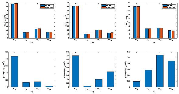
After the imputation methods were implemented, the mean and standard deviation of all data sets were calculated to determine whether the inherent structure of the data sets was modified. Figure 1 shows that the average and dispersion of the elements of the data sets were preserved even after carrying out the combination of imputation methods. However, it is worth noting that the performance of the imputation methods is generally dependent on the characteristics of the gap and the type of variable under study [40].
Figure 1. (a) Mean (b) median and (b) standard deviation of the collected data sets before and after undergoing the imputation stage, and the absolute value of their respective differences, (d), (e) and (f), before and after undergoing the imputation stage.
Figure 2 shows the sample of the plot of the imputed datasets of NO2, O3, PM10 and PM2.5 concentration levels.
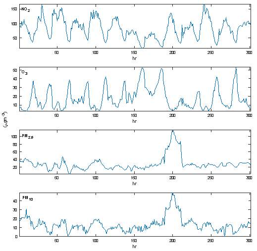
Figure 2. Plots of the imputed air pollutant concentrations, (a) NO2 (b) O3 (c) PM2.5 and (d) PM10, for the training period of 20 December to 31 December 2015
2.4 Data normalisation
Variables with large magnitudes have the tendency to mask those with small ones which might create some discrepancies in the results of a given model [41]. As such, the input data must be transformed to a smaller range of values to avoid the issue. This study employed the following formula that transforms the inputs to values ranging from 0 to 1, see Eq. (2):
| xi, norm=xi- xi, minxi, max-xi,min | (2) |
where
xi,min
and
xi,max
are the minimum and the maximum of the variable
xi
. Other available data normalisation techniques are described in detail in Hagan et al. [42].
2.5 ANN modelling
This section presents the underlying concepts that are essential in the development of the models in this study.
2.5.1 MLP network topology
An MLP model is a feedforward ANN which is composed of at least three layers of interconnected nodes: the input, hidden and output layers. Figure 3 shows a general architecture of an MLP network. The number of nodes in the input layer depends on the number of input variables, i.e. model predictors, while the output layer usually consists of a single node to provide the network estimate. The hidden layers collect the weighted sums of the information from the input layer and maps them to the output layer through the transfer function
σ
in layer
l=1, 2, …, Nh
where
Nh
is the number of hidden layers. The feedforward process can be mathematically expressed by Eq. (3):
| x̂j,t=σ∑i=1Nwj,il∙xi,t+bjl, j=1, 2, …, k, | (3) |
where
xi,t= x1,t x2,t … xN,t
are the values from the input nodes, k is the number of nodes in the hidden layer, N is the number of nodes in the input layer,
x̂j,t
is the output value of node j at time t, and
wj,il=wj,1l wj,2l … wj,Nl
and
bjl
are the weighting and bias constants of nodej, respectively. The single node in the output layer computes its output
in a similar fashion, see Eq. (4):
| yt=σ∑j=1kwil∙x̂j,t+bjl. | (4) |
Transfer functions are utilised to ensure that the outputs of the hidden and output layers have a continuous first-order derivative that can be utilised in calibrating the ANN weights and biases via the Back-Propagation (BP) algorithm [43]. BP in feedforward ANNs moves backward from the network error through the outputs, weights and inputs of each layer, and calibrates those weights carefully for a portion of the error by computing their partial derivatives
∂E/∂w
, or the relationship between their rates of change. Those computed derivates are then utilised by a learning rule, e.g. gradient descent, to calibrate the weights up or down whichever direction decreases the error. Table 2 lists some of the common activation functions and their properties. In this study, hyperbolic tangent and identity transfer functions were used in the hidden and output layers, respectively. On the other hand, there can be one, or several hidden layers, with a multiple number of neurons, although usually one hidden layer is employed in most applications. An iterative scheme was implemented to determine the optimal number of hidden neurons,
nh
, in hidden layer
l
, see Section 3.2.2.
Table 2. Common transfer functions and their properties
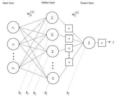
Figure 3. General MLP network architecture
2.5.2 Recurrent Neural Networks
RNNs are special types of neural networks sharing the information-processing features of an MLP network, with the addition of a mechanism that allows some output neurons to be connected to the neurons of the preceding layers. RNNs are distinguished from feedforward networks in that the feedback loops are connected to their previous outputs, allowing them to reveal and store sequential information from the input data in their recurrently hidden layers. These feedback mechanisms allow RNNs to preserve the sequential information of the input data in the hidden layers.
RNNs are trained using a modified version of the BP algorithm called Back-Propagation Through Time (BPTT). BPTT is an extension of the BP algorithm that can link one time step to the next, allowing RNNs to preserve sequential information. One downside in training RNNs is the vanishing gradient problem where the gradient update term becomes so small that no update takes place and the network parameters do not converge. In order to preserve the memory of the data in the current state of the model, gating systems that are inherently present in LSTM units are implemented. Such gating systems allow neurons to forget or pass memory if it is not being used, thus preserving enough error to allow updates [33].
2.5.3 LSTM
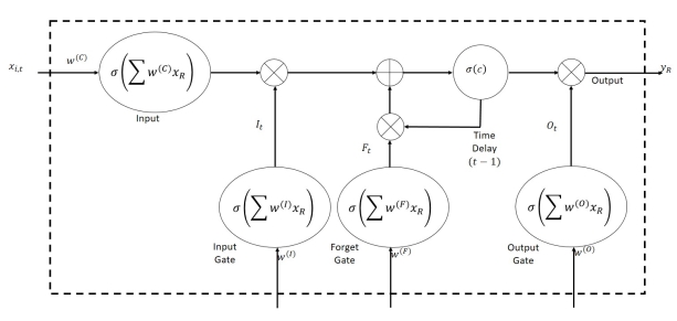
LSTM units are variants of RNNs that consist of one input layer, one output layer, and a series of memory blocks. Each block is composed of one or more self-recurrent memory cells and three multiplicative units, i.e. input, output and forget gates, that provide continuous analogues of read, write and reset operations for the blocks. An LSTM memory block with a single cell is illustrated in Figure 4.
The input gate enables incoming information to modify the state of the nodes, while the output gate permits or impedes the cell state from affecting other neurons. Furthermore, the forget gates were designed to learn and reset memory cells once their status is out of date, thereby preventing the cell status from growing without bounds and causing saturation of the transfer functions. The forward training process of an LSTM unit can be formulated as described in Eqs. (5)-(9):
| Ft=σw(F)∑i=1Nht-1∙xi,t+b(F) | (5) |
| It=σw(I)∑i=1Nht-1∙xi,t+b(I) | (6) | |
| ct=Ft∙ct-1+It∙ σw(C)∑i=1Nht-1∙xi,t+b(C) | (7) | |
| Ot=σw(O)∑i=1Nht-1∙xi,t+b(O) | (8) | |
| ht=Ot∙σct | (9) |
where
It
,
Ot
, and
Ft
are the outputs of the input, output and forget gates at time
t
, respectively,
ct
and
ht
represent the activation vector for each cell and memory block, respectively,
σ
denotes the transfer function, and
w
and
b
are the weighting and bias constants.
Figure 4. Network structure of an LSTM NN memory block with a single cell
3. Results and Discussion
This work aims to validate the performance of a deep RNN, called the LSTM model, in predicting hourly NO2, PM2.5 and PM10 pollution levels from 12 to 36 hours in advance. All computations were carried out using MATLAB R2018a software.
3.1 Model performance evaluation
To assess the performance of the models, the following statistical descriptors were employed: a) Root Mean Squared Error (RMSE), serving as the loss function during the network training, b) Coefficient of determination (r2), describing the association between the model predicted and actual values, and, c) Fractional Bias (FB), measuring the tendency of the model to over- or under-predict, given by Eq. (11), (12) and (13), respectively:
| RMSE=1NS ∑t=1Nsŷt-yt2 | (11) | |
| r2=1NS-1∑t=1NSŷt-μ̂σ̂yt-μσ2 | (12) | |
| FB=2μ-μ̂μ+μ̂, | (13) |
where
ŷt
and
yt
denote the t-th predicted and actual pollutant concentration values, respectively,
NS
is the number of samples, and
μ̂
,
μ
,
σ̂
and
σ
are the overall mean and standard deviation of the predicted and the actual pollutant concentration values, respectively.
3.2 Final parameter selection
3.2.1 Number of training epochs
The actual number of samples provided for training and testing was based on the prediction horizon, e.g. 12 to 36 hours in advance forecasts. Hence, the farther out the prediction, the fewer samples were available because of the time shifting required. The total amount of samples available for training and testing could be calculated as total samples, i.e. (8760 – h), where h is the prediction horizon. The number of training epochs was limited after reviewing training error values up to 250 training epochs for all prediction horizons, as seen in Figure 5. The optimum values of epochs were used for later model runs as they minimise the training error without overfitting. For the 12-hr prediction horizon task, optimum epoch values of 160, 240, 250 and 160 yielded the least average testing error on the prediction of NO2, O3, PM2.5, and PM10concentrations repeated three times, respectively. Furthermore, 160 epochs provided the least testing errors for the 24-hr ahead prediction of NO2 and PM10, while 250 and 190 epochs for O3 and PM2.5 pollutants, respectively. Lastly, 130, 240, 190 and 170 epochs resulted the least testing error for the 36-hr ahead prediction of NO2, O3, PM2.5, and PM10, respectively.
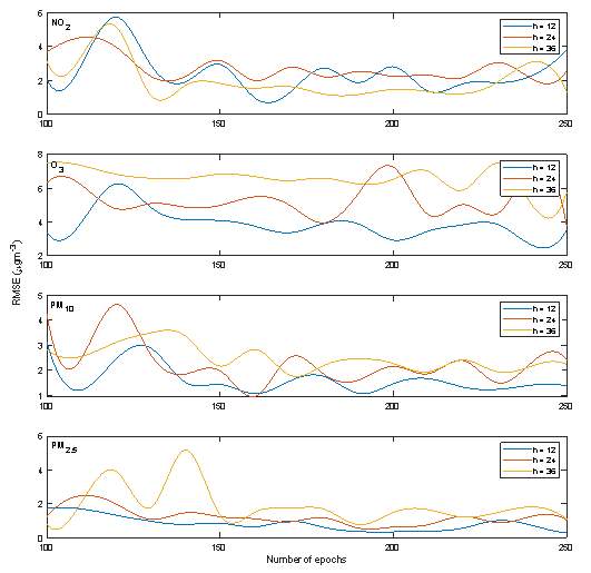
Figure 5. Number of epochs vs. the RMSE for test data sets for prediction horizons
3.2.2 Number of hidden units
A general method for finding the number of hidden layer and nodes in each layer remains unknown. Too many or too few hidden layers often lead to network overfitting or underperformance, respectively [42]. Consequently, the overall testing error of the models at various prediction horizons were tested against a varying number of LSTM hidden units in a single hidden layer. The results are shown in Figure 6. It can be observed that the networks employing 115, 250 and 160 hidden nodes yielded the least testing errors for 12-, 36-, and 24-hr NO2 prediction horizons, respectively. Additionally, 170, 190 and 130 hidden nodes resulted in the least testing errors for 12-, 36-, and 24-hr O3 prediction horizons, respectively, while 215, 120 and 180 hidden nodes provided the minimum testing errors for 12-, 36-, and 24-hr PM2.5 prediction horizons. Finally, 145, 125 and 210 hidden nodes provided the least testing errors for 12-, 36-, and 24-hr PM10 prediction horizons, respectively. These network configurations were utilised for later model runs.
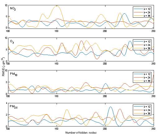
Figure 6.Number of hidden nodes vs. the RMSE for test data sets for different prediction horizons
3.3 Network performance with the optimal parameter configurations
Using the optimal values of the network parameters, the LSTM model was evaluated using the performance metrics that were described in Section 3.1. The performance evaluation results of all models are summarised in Table 3, where the labels “(1)” and “(0)” indicate the ideal values for r2 and FB, respectively.
Table 3. Performance evaluation results of the LSTM models
3.3.1 NO2 prediction
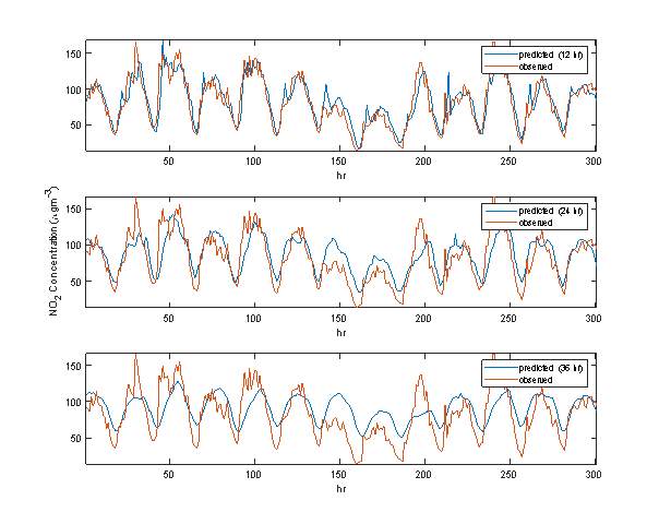
The models employed for the NO2 prediction tasks are labelled as M1, M2 and M3. Table 3 reveals that the model with the shortest prediction horizon, i.e. M1, provided the best forecasts of NO2 levels. In details, M1 provided the least testing error values (RMSE = 18.9688), while the one with the longest prediction horizon, i.e. M3, yielded the largest error (RMSE = 29.9918). Consequently, M1 can take into account approximately 88% of the variance of the observed NO2 values, achieving the best performance. The FB values also suggest that M1 has the least tendency (FB = 0.0096) to overestimate or underestimate NO2 predictions. The trends of the predicted values of NO2 using the LSTM model are shown in Figure 7.
Figure 7. Predicted vs. actual hourly values of NO2 for 300 hourly test training samples
3.3.2 O3 prediction
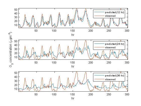
The models employed for the O3 prediction tasks are labelled as M4, M5 and M6. Table 3 shows that M4 provided the most accurate forecasts of O3 levels. M4 yielded the least error index (RMSE = 5.5431), outperforming models M5 (RMSE = 9.2886) and M6 (RMSE = 9.9933). Consequently, the same model was able to account approximately 85% of the variance of the observed O3 values, achieving the best performance. However, M6 provided the worst performance in terms of the r2 metrics by accounting only 35% of the variability of the observed O3 measurements. The results also reveal sudden drop in the r2 scores between M4 and M5, i.e. from 85% to 50%, as the prediction horizon increases from 12 h to 24 h. In terms of the FB metric, results suggest that model M4 provided the best PM2.5 predictions (FB = – 0.0343), while M6 the worst (FB = – 0.0416). Figure 8 illustrates the trends of the observed and predicted values of O3 using neural networks.
Figure 8. Predicted vs. actual hourly values of O3 for 300 hourly test training samples
3.3.3 PM2.5 prediction
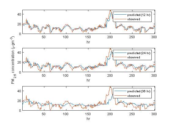
The models employed for the PM2.5 prediction tasks are labelled as M7, M8 and M9. M7 yielded the least error index (RMSE = 4.3742), outperforming all other models under the PM2.5 prediction task, i.e. M8 and M9, with RMSE scores of 5.0709 and 6.5990, respectively. Consequently, the same model can take into account approximately 82% of the variance of the observed PM2.5 values, achieving the best performance, while M9 is the worst (r2 = 49%). In terms of the FB metric, results suggest that M8 provided the best PM2.5 predictions (FB = – 0.0105). Figure 9 shows the trends of the observed and predicted values of PM2.5 the LSTM models.
Figure 9. Predicted vs. actual hourly values of PM2.5 for 300 hourly test training samples
3.3.4 PM10 prediction
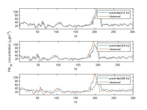
The models employed for the PM10 prediction tasks are labelled as M10, M11 and M12. The error indices indicate that M10 provided the most accurate forecasts of PM10 (RMSE = 7.3277), while M9 yielded the least accurate ones (RMSE = 11.9398). The results also show M10 can account for approximately 86% of the observed PM10 measurements, M11 approximately 77% and M12 only 56%. The FB results also indicate that M11 outperformed the rest of the models under PM10 prediction (FB = 0.0208). Figure 10 shows the trends of the observed and predicted values of PM10 using neural networks.
Figure 10. Predicted vs. actual hourly values of PM10 for 300 hourly test training samples
3.4 Comparison of the models
The performances of the LSTM models are compared with those of the benchmark feedforward MLP models. The MLP models were trained and tested using the same training and test sets and network hyperparameters, i.e. number of epochs, hidden layer and hidden units, applied for the LSTM models. Important results that are worth further discussion are shown in Table 4.
| LSTM | MLP | |||||||
| Code | RMSE | r2 (1) | FB (0) | Code | RMSE | r2 (1) | FB (0) | |
| NO2(t+12) | M1 | 18.9688 | 0.8752 | 0.0096 | M13 | 25.0426 | 0.7709 | 0.0244 |
| NO2(t+24) | M2 | 25.2094 | 0.7749 | 0.0389 | M14 | 30.5875 | 0.6364 | 0.0400 |
| NO2(t+36) | M3 | 29.9918 | 0.6774 | 0.0529 | M15 | 34.3202 | 0.5064 | 0.0511 |
| O3(t+12) | M4 | 5.5431 | 0.8529 | -0.0343 | M16 | 6.3867 | 0.7989 | -0.0379 |
| O3(t+24) | M5 | 9.2886 | 0.4952 | -0.0471 | M17 | 8.1246 | 0.6497 | -0.0535 |
| O3(t+36) | M6 | 9.9933 | 0.3530 | -0.0416 | M18 | 9.0256 | 0.5425 | -0.0666 |
| PM2.5(t+12) | M7 | 4.3742 | 0.8212 | 0.0305 | M19 | 4.4308 | 0.8145 | 0.0091 |
| PM2.5 (t+24) | M8 | 5.0709 | 0.7494 | -0.0105 | M20 | 5.2141 | 0.7342 | 0.0059 |
| PM2.5 (t+36) | M9 | 6.5990 | 0.4922 | 0.0213 | M21 | 5.6871 | 0.6609 | 0.0010 |
| PM10 (t+12) | M10 | 7.3277 | 0.8610 | 0.0223 | M22 | 8.6528 | 0.8246 | 0.0183 |
| PM10 (t+24) | M11 | 9.1576 | 0.7712 | 0.0208 | M23 | 9.6376 | 0.7612 | 0.0364 |
| PM10 (t+36) | M12 | 11.9398 | 0.5566 | 0.0450 | M24 | 9.9745 | 0.7267 | 0.0587 |
Table 4. Comparison of the performances between the LSTM and MLP models
3.4.1 NO2 prediction
The MLP models that were employed to predict NO2 levels across various prediction horizons are labelled as M13, M14 and M15. Table 4 shows that the LSTM models for NO2 forecasting performed better than the feedforward MLP models across all prediction horizons. For instance, M1 yielded better performance indices (RMSE = 18.9866, r2 = 0.8752 and FB = 0.0096, respectively) than those M13 (RMSE = 25.0426, r2 = 0.7709 and FB = 0.0244, respectively).
3.4.2 O3 prediction
The MLP models that were employed to predict O3 levels across various prediction horizons are labelled as M16, M17 and M18. It can be observed in Table 4 that the LSTM models only outperformed the MLP models in the 12 h – prediction of O3. For instance, M4 provided better performance indices (RMSE = 5.5431, r2 = 0.8529 and FB = – 0.0343) than M16 (RMSE = 6.3867, r2 = 0.7989 and FB = 0.0379). However, the LSTM models for both 24 – and 36 – hr prediction horizons, i.e. M5 and M6, respectively, underperformed in terms of RMSE and r2 metrics when compared with M17 and M18, see Table 4. The MLP models appear to be less affected by the sudden increase of prediction horizon, i.e. from 12 h (r2 = 0.7989) to 24 h (r2 = 0.6497), as compared with those of the LSTM models for O3 predictions.
3.4.3 PM2.5 prediction
The MLP models that were employed to predict PM2.5 levels across various prediction horizons are labelled as M19, M20 and M21. As revealed in Table 4, the LSTM models performed better than the MLP models in 12 – and 24 – hr prediction of PM2.5. For instance, M8 yielded better performance indices (RMSE = 5.0709, r2=0.7494 and FB = – 0.0105) than those of M20 (RMSE = 5.2141, r2 = 0.7342 and FB = 0.0059). However, M21 provided better forecasts of PM2.5 (RMSE = 5.6871, r2 = 0.6609 and FB = 0.0010) than M9 (RMSE = 6.5990, r2 = 0.4922 and FB = 0.0213).
3.4.4 PM10 prediction
The MLP models that were employed to predict PM10 levels across various prediction horizons are labelled as M22, M23 and M24. As compared with the results of the PM2.5 predictions, LSTM models outperformed the MLP models only for the 12 – and 24 – hr predictions of PM2.5. For instance, M11 provided better results (RMSE = 9.1576, r2 =0.7712 and FB = 0.0208) than M23 (RMSE = 9.6376, r2 = 0.7612 and FB = 0.0364). However, M24 provided more accurate predictions of PM10 (RMSE = 9.9745, r2 = 0.0.7267 and FB = 0.0587) than those of M12 (RMSE = 11.9398, r2 = 0.5566 and FB = 0.0450).
3.5 Deeper LSTM models
The ability of the deeper LSTM models was also examined in this study by considering an additional hidden layer to the existing models that have already been developed and described in Section 3.3, i.e. M1 through M12. The optimal hyperparameter configurations of M1 through M12 were also utilised in the training of the deeper LSTM models. The numerical results of the experiments are shown in Table 5, where labels M25 through M36 denote the deeper LSTM models across various prediction horizons per air pollutant.
Table 5 shows that the deeper LSTM models for NO2 predictions, i.e. M25, M26, M27, provided better results than their shallow counterparts, i.e. M1, M2 and M3. For instance, the performance indices of M5 (RMSE = 18.8347, r2 = 0.8788 and FB = 0.0219) are better than those of M1 (RMSE = 18.9688, r2 = 0.8752 and FB = 0.0096). However, the use of an additional number of hidden layers did not consistently improve the performance measures of the LSTM models. For instance, the deeper LSTM models for O3 predictions, i.e. M29 and M30, significantly outperformed M5 and M6, in terms of all performance indices except FB, while M28 failed to provide better results than M4, see Table 5. Furthermore, the deeper LSTM models for the PM2.5 and PM10 predictions, i.e. M31 to M36, failed to provide more accurate results.
| LSTM | Deeper LSTM | |||||||
| Code | RMSE | r2 (1) | FB (0) | Code | RMSE | r2 (1) | FB (0) | |
| NO2(t+12) | M1 | 18.9688 | 0.8752 | 0.0096 | M25 | 18.8347 | 0.8788 | 0.0219 |
| NO2(t+24) | M2 | 25.2094 | 0.7749 | 0.0389 | M26 | 20.4159 | 0.7851 | 0.0742 |
| NO2(t+36) | M3 | 29.9918 | 0.6774 | 0.0529 | M27 | 27.1383 | 0.7486 | 0.0659 |
| O3(t+12) | M4 | 5.5431 | 0.8529 | -0.0343 | M28 | 5.6180 | 0.8482 | -0.0248 |
| O3(t+24) | M5 | 9.2886 | 0.4952 | -0.0471 | M29 | 8.2725 | 0.6408 | -0.1085 |
| O3(t+36) | M6 | 9.9933 | 0.3530 | -0.0416 | M30 | 9.2161 | 0.5044 | -0.0624 |
| PM2.5(t+12) | M7 | 4.3742 | 0.8212 | 0.0305 | M31 | 4.3605 | 0.8206 | 0.0166 |
| PM2.5 (t+24) | M8 | 5.0709 | 0.7494 | -0.0105 | M32 | 6.3494 | 0.5632 | 0.0268 |
| PM2.5 (t+36) | M9 | 6.5990 | 0.4922 | 0.0213 | M33 | 7.1483 | 0.3582 | 0.0565 |
| PM10 (t+12) | M10 | 7.3277 | 0.8610 | 0.0223 | M34 | 7.5163 | 0.8609 | 0.0627 |
| PM10 (t+24) | M11 | 9.1576 | 0.7712 | 0.0208 | M35 | 11.9553 | 0.5638 | 0.0542 |
| PM10 (t+36) | M12 | 11.9398 | 0.5566 | 0.0450 | M36 | 12.8963 | 0.4481 | 0.0517 |
Table 5. Performance evaluation results of the LSTM models with two hidden layers
4. Conclusion
This paper examines the ability of an LSTM model to predict air pollutant concentrations based on historical air pollutant and time stamp data. LSTM models are RNNs with the ability to capture the long-time dependencies of time series data, making them the appropriate tools in short- and long-term air pollution applications. To evaluate the performance of the model, hourly concentration levels of NO2, O3, PM2.5 and PM10 from January to December 2015 were collected from the London Marylebone monitoring station in Central London. Twelve different models, i.e. three prediction horizons for each air pollutant, were trained and compared using the same dataset. The experimental results exhibited that the LSTM model outperformed the benchmark feedforward MLP models as indicated by the RMSE, FB and r2 performance indices provided that their architecture and training parameters are fine-tuned and optimised before the testing scheme. Consistent with the results of previous case studies and almost all forms of forecasting, the performance of LSTM models appears to degrade as the prediction horizon becomes farther. This is more significant especially in the models employed to forecast O3 and PM2.5. Furthermore, the graphs of the observed and predicted measurements of the air pollutants under study illustrate that the forecasted values are generally consistent with the actual data in most cases. However, slight to major deviations can be observed when extreme or peak values occur. These observations highlight the limitations even of deep neural network models in simulating peak pollution levels . The comparison of the LSTM models with the MLP models exhibits that neural network models with deep recursive architectures have better performances than the feedforward structures in most simulations. This finding is consistent with those of previous works including [30]. Finally, the results show that the deeper LSTM models failed to significantly improve the prediction power of the LSTM models, with the exception of forecasting NO2 levels. They indicate that the utilisation of extra hidden units may not be necessary and could have contributed to the complexity of the models leading to overfitting issues [41].
References:
[1] J. Colls, Air Pollution 2nd Edition. 29 West 35th Street, New York, NY 10001: Spon Press, 2001.
[2] Y. Zhang, M. Bocquet, V. Mallet, C. Seigneur, and A. Baklanov, “Real-time air quality forecasting, Part II: State of the science, current research needs, and future prospects,” Atmos. Environ., vol. 60, pp. 656–676, 2012.
[3] World Health Organization, “WHO | Ambient air pollution,” WHO, 2018. [Online]. Available: http://www.who.int/airpollution/ambient/en/. [Accessed: 10-Sep-2018].
[4] World Health Organization, “Review of evidence on health aspects of air pollution – REVIHAAP Project,” World Heal. Organ., p. 309, 2013.
[5] Organisation for Economic Co-operation and Development, “Policy Highlights – The economic consequences of outdoor air pollution,” 2016.
[6] European Commission, “New Air Quality Directive – Environment – European Commission.” [Online]. Available: http://ec.europa.eu/environment/air/quality/legislation/directive.htm. [Accessed: 10-Sep-2017].
[7] A. Baklanov et al., “Integrated systems for forecasting urban meteorology, air pollution and population exposure,” Atmos. Chem. Phys. Atmos. Chem. Phys., vol. 7, pp. 855–874, 2007.
[8] K. P. Moustris, I. C. Ziomas, and A. G. Paliatsos, “3-day-ahead forecasting of regional pollution index for the pollutants NO2, CO, SO2, and O3 using artificial neural networks in athens, Greece,” Water. Air. Soil Pollut., vol. 209, no. 1–4, pp. 29–43, 2010.
[9] Z. Jacobson, “Development and Application of a New Air Pollution Modeling System – II. Aerosol Module Structure and Design,” Atmos. Environ., vol. 31, no. 2, pp. 131–144, 1997.
[10] M. E. Chang and C. Cardelino, “Application of the Urban Airshed Model to forecasting next-day peak ozone concentrations in Atlanta, Georgia.,” J. Air Waste Manag. Assoc., vol. 50, no. 11, pp. 2010–2024, 2000.
[11] M. T. Chuang, Y. Zhang, and D. Kang, “Application of WRF/Chem-MADRID for real-time air quality forecasting over the Southeastern United States,” Atmos. Environ., vol. 45, no. 34, pp. 6241–6250, 2011.
[12] S. F. Mueller and J. W. Mallard, “Contributions of natural emissions to ozone and PM2.5 as simulated by the community multiscale air quality (CMAQ) model,” Environ. Sci. Technol., vol. 45, no. 11, pp. 4817–4823, 2011.
[13] M. A. Elangasinghe, N. Singhal, K. N. Dirks, and J. A. Salmond, “Development of an ANN–based air pollution forecasting system with explicit knowledge through sensitivity analysis,” Atmos. Pollut. Res., vol. 5, no. 4, pp. 696–708, 2014.
[14] A. K. Paschalidou, S. Karakitsios, S. Kleanthous, and P. A. Kassomenos, “Forecasting hourly PM10 concentration in Cyprus through artificial neural networks and multiple regression models: Implications to local environmental management,” Environ. Sci. Pollut. Res., vol. 18, no. 2, pp. 316–327, 2011.
[15] K. Y. Ng and N. Awang, “Multiple linear regression and regression with time series error models in forecasting PM 10 concentrations in Peninsular,” Environ. Monit. Assess., 2018.
[16] A. Russo, P. G. Lind, F. Raischel, R. Trigo, and M. Mendes, “Neural network forecast of daily pollution concentration using optimal meteorological data at synoptic and local scales,” Atmos. Pollut. Res., vol. 6, no. 3, pp. 540–549, 2015.
[17] B.-C. Liu, A. Binaykia, P.-C. Chang, M. Tiwari, and C.-C. Tsao, “Urban air quality forecasting based on multi- dimensional collaborative Support Vector Regression (SVR): A case study of Beijing- Tianjin-Shijiazhuang,” PLoS One, vol. 12, no. 7, pp. 1–17, 2017.
[18] N. Güler Dincer and Ö. Akkuş, “A new fuzzy time series model based on robust clustering for forecasting of air pollution,” Ecol. Inform., vol. 43, no. October 2017, pp. 157–164, 2018.
[19] Y. Bai, Y. Li, X. Wang, J. Xie, and C. Li, “Air pollutants concentrations forecasting using back propagation neural network based on wavelet decomposition with meteorological conditions,” Atmos. Pollut. Res., vol. 7, no. 3, pp. 557–566, 2016.
[20] M. Catalano and F. Galatioto, “Enhanced transport-related air pollution prediction through a novel metamodel approach,” Transp. Res. Part D Transp. Environ., vol. 55, pp. 262–276, 2017.
[21] H. T. Shahraiyni and S. Sodoudi, “Statistical modeling approaches for pm10 prediction in urban areas; A review of 21st-century studies,” Atmosphere (Basel)., vol. 7, no. 2, pp. 10–13, 2016.
[22] G. Grivas and A. Ã. Chaloulakou, “Artificial neural network models for prediction of PM 10 hourly concentrations , in the Greater Area of Athens , Greece,” Atmos. Environ., vol. 40, pp. 1216–1229, 2006.
[23] A. Rahimi, “Short-term prediction of NO2 and NO x concentrations using multilayer perceptron neural network: a case study of Tabriz, Iran,” Ecol. Process., vol. 6, no. 1, p. 4, 2017.
[24] P. Jiang, Q. Dong, and P. Li, “A novel hybrid strategy for PM2.5 concentration analysis and prediction,” J. Environ. Manage., vol. 196, pp. 443–457, 2017.
[25] M. . Gardner and S. . Dorling, “Artificial neural networks (the multilayer perceptron)—a review of applications in the atmospheric sciences,” Atmos. Environ., vol. 32, no. 14–15, pp. 2627–2636, 1998.
[26] C. Capilla, “Multilayer perceptron and regression modelling to forecast hourly nitrogen dioxide concentrations,” WIT Trans. Ecol. Environ., vol. 183, pp. 39–48, 2014.
[27] M. Catalano, F. Galatioto, M. Bell, A. Namdeo, and A. S. Bergantino, “Improving the prediction of air pollution peak episodes generated by urban transport networks,” Environ. Sci. Policy, vol. 60, pp. 69–83, 2016.
[28] J. Fan, Q. Li, J. Hou, X. Feng, H. Karimian, and S. Lin, “A Spatiotemporal Prediction Framework for Air Pollution Based on Deep RNN,” vol. IV, pp. 7–9, 2017.
[29] T. Li, H. Shen, Q. Yuan, X. Zhang, and L. Zhang, “Estimating Ground-Level PM2.5 by Fusing Satellite and Station Observations: A Geo-Intelligent Deep Learning Approach,” Geophys. Res. Lett., vol. 44, no. 23, p. 11,985-11,993, 2017.
[30] X. Li, L. Peng, Y. Hu, J. Shao, and T. Chi, “Deep learning architecture for air quality predictions,” Environ. Sci. Pollut. Res., vol. 23, no. 22, pp. 22408–22417, 2016.
[31] Z. Qi et al., “Deep Air Learning: Interpolation, Prediction, and Feature Analysis of Fine-grained Air Quality,” no. 38, 2017.
[32] F. Biancofiore et al., “Recursive neural network model for analysis and forecast of PM10 and PM2.5,” Atmos. Pollut. Res., vol. 8, no. 4, pp. 652–659, 2017.
[33] S. Hochreiter and J. Schmidhuber, “Long Short-Term Memory,” Neural Comput., vol. 9, no. 8, pp. 1735–1780, 1997.
[34] B. S. Freeman, G. Taylor, B. Gharabaghi, and J. Thé, “Forecasting air quality time series using deep learning,” J. Air Waste Manage. Assoc., vol. 68, no. 8, pp. 866–886, Aug. 2018.
[35] X. Li et al., “Long short-term memory neural network for air pollutant concentration predictions: Method development and evaluation,” Environ. Pollut., vol. 231, pp. 997–1004, 2017.
[36] BBC News, “London hits annual air quality limit in one month – BBC News,” 2018. [Online]. Available: https://www.bbc.co.uk/news/uk-england-london-42877789. [Accessed: 11-Jun-2018].
[37] Department for Environment Food and Rural Affairs, “Defra, UK.” [Online]. Available: https://uk-air.defra.gov.uk/. [Accessed: 23-Apr-2017].
[38] P. J. Santos, A. G. Martins, and A. J. Pires, “Designing the input vector to ANN-based models for short-term load forecast in electricity distribution systems,” Electr. Power Energy Syst., vol. 29, pp. 338–347, 2007.
[39] K. H. Li, N. H. U. D. Le, L. I. Sun, and J. V Zidek, “SPATIAL ± TEMPORAL MODELS FOR AMBIENT HOURLY PM 10 IN VANCOUVER Spatia-Temporal Models for Ambient Hourly PM10 in Vancouver,” Environmetrics, vol. 338, no. March, 1999.
[40] H. Junninen, H. Niska, K. Tuppurainen, and J. Ruuskanen, “Methods for imputation of missing values in air quality data sets,” vol. 38, pp. 2895–2907, 2004.
[41] S. Samarasinghe, Neural Networks for Applied Sciences and Engineering. Taylor & Francis, 2006.
[42] M. T. Hagan, H. B. Demuth, and M. H. Beale, “Neural Network Design,” Bost. Massachusetts PWS, vol. 2, p. 734, 1995.
[43] C. M. Bishop, Pattern Recognition and Machine Learning, vol. 53, no. 9. 2013.
[44] C. M. Bishop, Neural Networks for Pattern Recognition. New York, NY, USA: Oxford University Press, Inc., 1995.
Cite This Work
To export a reference to this article please select a referencing stye below:
Related Services
View allRelated Content
All TagsContent relating to: "Environmental Studies"
Environmental studies is a broad field of study that combines scientific principles, economics, humanities and social science in the study of human interactions with the environment with the aim of addressing complex environmental issues.
Related Articles
DMCA / Removal Request
If you are the original writer of this dissertation and no longer wish to have your work published on the UKDiss.com website then please:


