Deterioration of Soil Strength Due to Dynamic Pore Water Pressure
Info: 16614 words (66 pages) Dissertation
Published: 13th Dec 2019
Tagged: Environmental ScienceEcology
AN INVESTIGATION INTO THE DETERIORATION OF SOIL STRENGTH DUE TO DYNAMIC PORE WATER PRESSURE VARIATIONS ON FINSBURY PARK STATION EARTHWORKS
1 Introduction
Transportation infrastructure provides an important service to the modern world and has done for centuries. Transport links allow regions to develop economically by allowing the ease of movement of people and goods and they also have huge significance on a political and social level.
Due to the importance of transportation infrastructure, it is important that all structural components are regularly assessed and repaired in accordance with the outcome of the assessments because, in the event of failure of transportation infrastructure, huge economical costs and social disruption can be expected.
A key structural component of transportation infrastructure are earthworks. These are employed to improve the efficiency at which people and vehicles can travel from destination to destination by providing more even gradients and improving ride quality. Therefore, it is evident that the failure of this structural component has the potential to bring transportation infrastructure to a standstill. It is important to investigate how the likelihood of these failure mechanisms occurring can be decreased so that the designed lifetime capacity of earthworks can be utilised entirely. It is for this reason that this research dissertation has been undertaken with the collaboration of Network Rail, Transport for London and the Author.
This dissertation research project will focus on the interaction of transportation infrastructure earthworks with the environment, looking particularly at the effect of dynamic pore water pressure variations and the subsequent effects that this can have on strength of soil. The research will also extend wider by looking at the other possible environmental interactions that could be considered and their relative influence on soil property variations.
1.1 Aims and Objectives
The aim of this research project is to investigate the effect of cyclical pore water pressure loading variations on samples of London Clay using a triaxial test under CU conditions.
The following objectives have been set by the author in order to meet the aim, which are:
- To investigate and undertake a literature review of the history of earthworks and the environmental factors that could affect soil strength, looking particularly at dynamic pore water pressure variations and reviewing existing theory on the assessment of soil strength.
- Collect field data and specimens through industrial collaboration and benefit from representative samples.
- Undertake a wet sieve test and hydrometer test to assess the particle size distribution of the samples and confirm soil classification.
- Design and undertake a laboratory experiment using representative samples using a triaxial test under CU conditions to assess the control failure strength.
- Undertake laboratory experiments using reconstituted samples to analyse the relationship between pore water pressure variations and subsequent soil failure strength.
1.2 Research Methodology
The author will initially undertake a review of the current literature to collect primary source data in relation to the interaction of the environment with soil properties. This will subsequently extend into looking principally at the effect of dynamic pore water pressure variations and undertaking simultaneous exploration on similar thesis’ that have looked specifically at this aspect of soil mechanics.
Proceeding the literature review, preparation will be undertaken to set up a laboratory experiment. Partially-disturbed samples will be collected from Finsbury Park Railway Station, London, United Kingdom and up to 9 samples will be tested using the triaxial test under CU conditions. Due to the time constraints involved in the project, it is only possible to undertake a laboratory experiment under CU conditions because a consolidated drained test would take considerably longer.
Continuing the laboratory experiments, the results will be presented both graphically and quantitatively in the succeeding section. It will then be determined, in a discussion, whether a relationship can be seen between dynamic pore water pressure loadings and soil specimen failure strength through the analysis of the results section.
2 Literature Review
2.X History of Transportation Infrastructure Earthworks
Nowak and Gilbert (2015) explained that the first instance of transportation earthwork construction occurred around 2000 years ago in the Roman era with the construction of Roman roads, in which the roads were constructed using a compacted engineered fill or stone with gravel and pebbles placed on top, which exploits the classic soil mechanics theory and applications that are used today. However, up until the industrial revolution, there was limited earthworks construction in the UK. Manolopoulou (2009) stated that the changes in the organization of the UK manufacturing industry transitioned the UK from a rural to an urban economy and so a transportation revolution resulted.
Nowak and Gilbert (2015) produced the adopted table shown in Figure 1 which denotes a timeline of earthwork construction progression for transportation earthworks during the industrial revolution for railways, highways and canals and this shows each transportation group being developed for the passage of commercial goods.
Development of these transportation networks carried on through the end of the 19th century to the end of the 20th century. Perry et al (2003) stated that peak construction of canals, railways and highways earthworks were in the 1800’s, 1850’s and 1970’s respectively and this had an influence on the method of construction and material that was used.
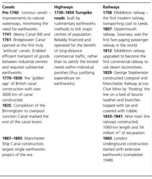
Figure X: A timeline of earthwork construction during the Industrial Revolution (Nowak and Gilbert, 2010)
2.X Earthworks Method of Construction
Earthwork construction methodology has vastly changed from the start of the industrial revolution until the present day which can be attributed to factors such as an improved knowledge of classic soil mechanics theory, lessons learned and the development of materials/plant available. With different types of transportation infrastructure earthworks being constructed during different time periods, it can be assumed that the construction methodology between railways, highways and canals would be significantly different as well as their properties and behaviours equally.
For example, Briggs et al (2016) elaborate on the comparison between railways and highway embankments by describing the process used during railway embankment construction as being built empirically and without geotechnical design experience. O’Brien et al (2007) explains that embankments constructed using the excavated materials from railways cuttings results in the earthworks being made up of a clod matrix clay fill, as shown in Figure X. This is in comparison to highway embankments which were constructed a significant period after railway embankments and used the experience from the construction of railway embankments to improve the construction methodology. AASHTO (2008) explains the common method of construction includes the removal of topsoil and incremental layering of 250mm layers. Additionally, a report by Mott MacDonald (2011) supports how road embankments are constructed in compacted layers with sufficient drainage whereas Skempton (1996) describes how railway embankments were constructed using a methodology called end-tipping which inhibits the consolidation of soil through compaction of lower layers.
Skempton (1996) elaborates further by reciting that during the time periods considered during peak railway construction, navvies sourced the embankment fill from cuttings that had been excavated using a pick and shovel. This fill was then used to create an embankment by end-tipping off the end of the limit of the cutting, as shown in Figure X. In the 1840s, Skempton (1996) explains that John MacNeill had identified that, for clay, it would be reasonable to compact the embankment in 4ft layers to allow consolidation of the excavated material. However, this was deemed to be too slow a process, so end tipping continued to be performed as common practise.
The practice of differing methods of construction has an effect on the temporal behaviour of an earthwork, which in many cases is detrimental. The failure of an earthwork element can have a huge social and economic impact because transportation infrastructure earthworks are crucial infrastructure assets and the populace’s daily endeavours depend upon them. The difference in construction methodology is represented in the number of relative geotechnical failures in railways compared to highways, where Perry (2003) describes how the cost of earthwork maintenance and renewals is the equivalent of £18,000/km in railways and £5700/km in highways. Slope stability analyses can take the properties of an earthwork asset including the material composition and soil strength values to create a series of failure mechanisms that are analysed independently to determine the proximity of the critical failure mechanism to the factor of safety specified.
2.X Slope Stability
Slope stability analyses utilise the ultimate shear strength of a soil to assess the condition of a slope under certain conditions. The ultimate shear strength of a soil can be determined through laboratory testing in the form of; the direct shear test, the triaxial compression test, the unconfined compression test or the vane shear test.
The parameters that are used in a slope stability analysis depends on the soil that is being investigated, in addition to whether the analysis is being carried out under short term or long terms conditions and the in-situ conditions, such as total stresses and pore pressures, that it is subject to. A change these parameters has a direct influence on the strength capacity of a large soil mass, such as embankments. These values are normally consistent over short time periods but interactions with the environment can cause them to change. For example, heavy and intense precipitation can increase the pore water pressures in the soil which results in a decrease in effective stresses in a short term drained analysis. This results in shear strength of a soil being decreased which is an unfavourable scenario. There can also be environmental considerations that look at the microstructure of a soil mass such as chemical interactions.
It is important to understand the drivers and influences on earthwork slope stability, especially in railways. These influences can have both a beneficial and detrimental effect on the soil properties and influences how close these embankments are to the critical failure mechanism, which may vary on both a spatial and temporal scale as the extent of proximity to the critical failure mechanism is dynamic.
2.X Soil-Environment Interfaces
Gens (2010) explains, in concurrence with the subsequent authors of literature in this section, how modern geotechnical engineering complexity arises from the interaction of soil with the environment and gives an example of how soil environment conditions such as low temperatures fluctuating above and below zero degrees can cause cyclic freezing of the ground which can affect soil characteristics.
It is evident in the in the literature that environmental drivers can have a considerable effect on soil properties when looking at both the embankment as a whole, such as pore water pressure variations and vegetation ingress. It is also possible that environmental drivers can affect the microstructure of a soil mass, such as chemical contamination ingress and the effect of cyclical loading. It is important that the distinction between complete soil mass and a soils local microstructure are understood and the subsequent environmental drivers will be explained in the following sections with this in mind.
2.X.X Pore Water Pressure
It is possible for environmental parameters to vary on a temporal scale as well as vary in terms of magnitude. For example, a soil’s organic composition may not change dramatically with time compared to pore water pressures, which can vary over shorter periods of time and affect the whole mass of soil.
2.X.X.X The Relationship Between Pore Water Pressure and Soil
Pore water pressures have a direct contribution to stresses “felt” by the soil, these are known as effective stresses. These effective stresses are directly associated with the shear strength of soils, τ , as will be explained in greater detail in section 2.X (Terzaghi, 1925). Mitchell (1960) explains how pore water pressures in a soil mass are made up of four components:
- Elevation pressure
- Hydrostatic forces
- Clay particles suction pressure
- Added osmotic pressure
Where elevation pressure is normally the most influential type of pore water pressure within a soil mass because its pressure depends on the volume of water that is above a specific locus. Mitchell (1960) explains how the remaining types of pore water pressure are normally assumed to be negligible in geotechnical analysis in comparison the elevation pressure, but only under static conditions.
2.X.X.X Cohesive and Non-Cohesive Soils
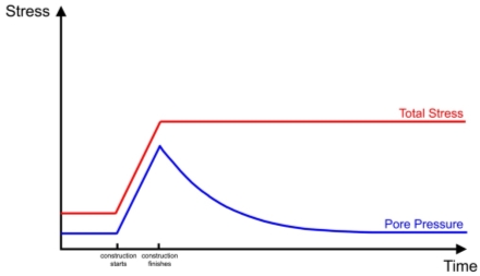
The responses to the influence of pore water pressure changes within cohesive and non-cohesive soils are different, and this can have a dramatic effect on the shear strength of soils during different phases. In the case of a surcharge load, it is possible for cohesive soils, such as clay, to see an instantaneous and short term increase in pore pressure as the internal water within pores of cohesive soils are unable to dissipate. This leads to the increase in internal pore water pressures, otherwise known as excess pore water pressures (Skempton, 1954). These pore pressures are hydrostatic forces, as indicated in section X.X, which results due to the soil skeleton wanting to change in volume but is prevented by the equal and opposite force from the hydrostatic forces (Bobet, 2003). These pore pressures then dissipate with time back to their equilibrium pore water pressures as time increases, this is shown in Figure X.
On the other hand, non-cohesive soils are able to dissipate internal water pressures instantaneously when subject to an external surcharge load, resulting in no excess pore water pressures being induced within the soil mass in the short term or long term and therefore, pore water pressures are constant.
Figure 1: A graph representing the change in total and pore water pressures post construction. Note: It has been assumed no pore water dissipation occurs during the construction phase.
Barnes (2010) explains how these two conditions exhibited during the short term between cohesive and non-cohesive soils impacts the method of analysis undertaken. Therefore, to assess the effect of pore water pressures in the short term for cohesive soils, an undrained analysis is undertaken and for a non-cohesive soil, a drained analysis is almost always undertaken. This will be explained further in section X.X
2.X.X.X Embankment Loading and Cutting Unloading
Figure X above represents a scenario of loading on a soil mass to induce excess pore water pressures that subsequently dissipate. This would be possible in the construction of an embankment. However, it is also possible that pore water pressures can be locked in t
2.X.X.X Pore Water Pressure Distribution within an Embankment
There is a larger likelihood for pore water pressures in a railway embankment to vary more dramatically due to various parameters. Firstly, due to the absence of horizontal pressures from adjacent soil on the sides of an embankment, there is a difference in drainage path length (Terzaghi, 1943). This means that pore water pressures can alleviate themselves by dissipating water into atmospheric conditions horizontally and do not have to specifically move vertically. It is unlikely for a railway embankment to display a distinct ground water table because it is elevated from ground level, where you are unlikely to have a ground water table above. However, it is possible for pools of water to move into a railway embankment, which is typical to their clod-matrix characteristics from construction methods, as explained in section X.X. Rushton and Ghataora (2012) explain how the ballast on railway tracks had a high permeability ratio and is designed to that drainage from the surface is rapid into the subgrade beneath. Track maintenance and renewal incorporates a graded surface into the ballast and subgrade materials so that drainage can exit either side and down the sides of the embankment. However, during the construction phase and the subsequent years of use, ballast was laid down flat which would have causes pooling of water beneath the railway tracks and would have subsequently infiltrated the embankment.
Additionally, due to the location of the embankment in question, it would also be possible that flooding of the surrounding area could occur, which would increase pore water pressures within the embankment by incorporating a ‘new’ ground water table into the analysis. Greater London Authority (2011) identified Finsbury Park as a place of significant flood risk, especially around the station because the location is the lowest point in the borough and has a poor drainage system.
2.X.X.X Effect of Vegetation on Pore Water Pressure
The effect of vegetation on the slopes is described by Ishak et al (2013) as being split into two categories, mechanical and hydrological. They explain how roots and vegetation can affect the strength of a soil mass through a mechanical reinforcement mechanism, where the roots bind the soil together. As deformation occurs, tensile stresses will be induced in the root which will subsequently reduce the stresses felt by the soil. In relation to the influence on pore water pressures, Charlatfi (2014) explains that roots can also induce suction pressure in a slope and it was found that moderately small suction changes from 18kPa to 39kPa can increase the safety factor against failure of the slope but also affect the presence of water within the embankment by converting water mass from the embankment to water vapour from its leaves using the process of evapotranspiration. However, this environmental factor has a predominantly beneficial effect to the stability of a slope and therefore I will not be pursuing this further within my research.
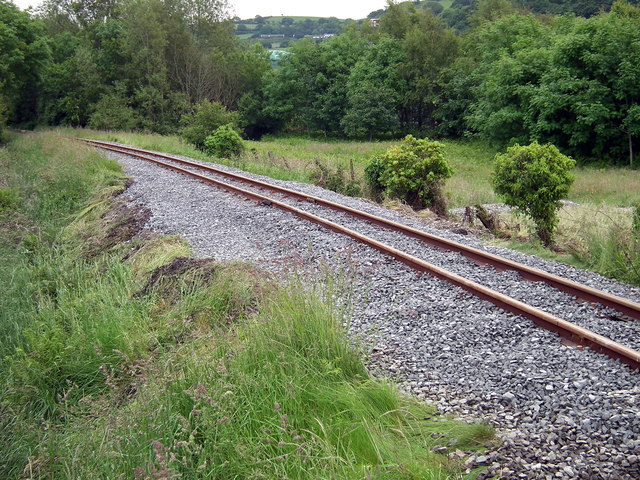
Figure 2: Vegetation Growth on a railway embankment in Wales (Lucas, 2012)
Endo (1980) expands on Charlatfi’s theory by detailing two further vegetation mechanisms that can affect soil strength. He explains how the vegetation can perform as an additional load on an embankment, in particular trees, where the critical location would be at the crest of an embankment compared to the toe of the embankment. This would provide additional driving forces that would affect the strength of a soil mass. An additional factor, detailed by Endo (1980) is the effect of wind on vegetation, as it can induce shear forces and moments locally to the embankment. However, this factor only provides an isolated effect to the embankment strength and will not be pursued further in this investigation.
2.X.X.X Temporal Variations
Events such as flooding, heavy rainfall and changes in the ground water table induce dynamic pore water pressures variations with an embankment mass which has an effect on the embankment as a whole. These variations cause a cycling of the effective stresses within the embankment and produce cycles of shrinking and swelling for a clay sample as the cohesive soil responds to the change in effective stress. Lee and Focht (1975) explains how clay soils can develop progressive strains due to pulsating stresses, where soil failure strength is reduced in comparison to static conditions (Lee and Focht, 1975). Therefore, the author is proposing that the effect of a cyclical nature of pore water pressures variations could potentially result in a decrease in ultimate failure strength.
Many studies have been undertaken to assess the dynamic pore water pressure conditions during short term loading (ie. earthquakes) on cohesive soils (Seed, 1966; Biondi, 2007; Bobet, 2003; Lamri and Hidjeb, 2008). This short-term loading symbolises that the experimental approach prohibited the drainage of pore water pressures therefore the author is proposing to undertake an experiment that would look at the effect of the cyclical pore water pressure variations under drained conditions and assessing the impact on failure strength of the soil.
In summary of the soil-environment interface literature, it is evident that the effect of chemical and cyclical loading are local effects in comparison to the scope of an entire embankment earthwork. Therefore, the author is proposing they will not be pursued further within this investigation. On the other hand, pore water pressures present alterations to the entirety of an earthwork asset.
This paper will therefore focus on the effect of pore water variations within railway embankments, looking particularly at the effect of cyclical variations on soil parameters. These soil parameters and their existing theories will be explained in the subsequent sections.
2.X.X Additional Considerations – Cyclical Loading and Chemical Ingress
Looking particularly at transportation infrastructure earthworks, it is logical to assess the effect of loadings. All transportation earthworks have been commissioned to carry transportation vehicles, therefore a load is applied at the top of the bank. For example, on railway infrastructure, loading is cyclical is large, dynamic surcharges are applied and removed, as shown in Figure X.
Figure X: Dynamic Surcharge Load on Crest of Earthwork (DBM, 2010)
Mott Macdonald (2011) explained that train axle loads apply an elastic strain to the embankment however there may also be irrecoverable plastic strains experienced by the embankment. The report details an investigation by Selig and Sluz (1978) and Yoo and Selig (1979) in which they conclude that irrecoverable plastic strains can accumulate over a large number of cycles. The plastic strains correspond to yielding within the clay samples and this can result in a change in the stiffness of the sample and swelling in early stages of deformations. This results in a modification of the inter-particle microstructure of the soil through work being done (Graham et al, 1983). Mott Macdonald (2011) explained in their report this aspect highlighted an evident gap in the literature in that only static loadings had been considered in previous research and that no research had been carried out on existing railway embankment fill specimens.
Table X, adopted from Esveld (2001) provides a summary of the train axle loading configurations that could be experienced on Britain’s railway transportation infrastructure.
| Rolling Stock | Number of Axles | Empty Weight/Axle (kN) | Loaded Weight/Axle (kN) |
| Light Rail | 4 | 80 | 100 |
| Passenger Train | 4 | 100 | 120 |
| Locomotive | 4 or 6 | 215 | – |
| Freight Wagon | 2 | 120 | 225 |
Table 1: A table showing train axle loadings on Britain’s railway infrastructure (Esveld, 2011)
This table presents the largest axle weight at 120kN which is transferred to the embankment via rails, sleepers and ballast (Mott Macdonald, 2011). This stress path permits the lowest pressure to be felt by the embankment for the force by dissipating the stress over a larger area.
The Boussinesq stress distribution theory, of a point load below the surface, describes how these stresses are dispersed across a wider area as depth increases (Boussinesq, 1885). Therefore, any effects of cyclical loading would be concentrated in the crest of the embankment and not the embankment mass entirely.
On another note, studies into the interaction of chemicals with soil structure has been undertaken by Ramiah et al (1970), where they established a relationship between chemical interactions and peak residual strength. Chemicals that interact with soils have the potential to perform as flocculants or dispersants which represent their ability to promote the clumping of particles and prevent the clumping of particles through dispersion, respectively. Their findings demonstrate how the interaction of a chemical that promotes flocculation will adjust a soil’s microstructure and result in a higher peak residual strength.
BBC News (2015) recently undertook an investigation that revealed that 10% of Britain’s railway infrastructure dispose their toilet waste directly onto the tracks along with the sterilization chemicals that are mixed before disposal. These chemicals have the likelihood of percolating through the ballast into the subgrade below and interacting with the soil in the means explained by Ramiah et al (1970).
2.X Soil Mechanics Theory
2.X.X Total and Effective Stresses
The total stress of a soil is the stress that is applied to a plane when assuming the soil to be a solid material where vertical stresses (σV) act on the horizontal plane of a soil element and where horizontal stresses (σH) act on the vertical plane of a soil element, however these horizontal and vertical stresses are not always in equilibrium (Barnes, 2010).
Vertical stresses can be found by taking the bulk unit weight (γb) of the soil above a soil element and multiplying by the depth (z) to obtain the total stress, as shown below:
[ 1 ]
σV= γb.z
However, pore water pressures within soil samples can convert these stresses into hydrostatic forces, thereby making the soil ‘feel’ an effective stress. The principle of the effect of pore water pressures in soil mechanics was first discovered by Terzaghi (1925), who realised that total stresses were made up of two components; intergranular stress, σg, and pore water pressure, u. This gives the effective stress equation shown in Equation X.
[ 2 ]
σ’= σ-u
In comparison, the vertical stresses, horizontal stresses cannot be obtained from bulk unit weights of adjacent soils because these stresses act normal to the direction of acceleration due to gravity (g). Instead, soils demonstrate coefficients of earth pressure, K0, which varies dependant on the soil type and looks particularly at a soil state when at rest (i.e. a soil in its natural undisturbed state). Brooker and Ireland (1965) explain how a normally consolidated clay has a K0 value which is calculated dependent on the friction angle (ϕ’), as shown in Equation X.
[ 3 ]
K0,NC=0.95-sin(ϕ’)
This earth pressure coefficient is then used to determine the horizontal stress acting on the vertical plane of a soil element using Equation 3.
[ 4 ]
σH’=K0,NC.σV’
However, in the case of embankments, equations X and X do not fully represent the horizontal and vertical stresses because of the influence of the shape of the embankment and the loss of soil mass either side of the embankment, which results in less horizontal constriction and therefore lower horizontal stresses.
2.X.X Mohr Coulomb Theory
Mohr-Coulomb theory demonstrates how an isotropic material will fail under major and minor principal stresses and works on the assumption that failure only depends on the principal stresses, the shape of the failure line, the location of the principal stresses and the shear acting on the failure plane (Labuz and Zang, 2012; Mohr 1900).
It was Coulomb who initially proposed that there was a relationship between these variables through Equation X, where τ is the shear stress, c’ is the cohesion intercept and σN is the stress perpendicular to the shear plane (Heyman 1972).
[ 5 ]
τ=c’+ σNtan(ϕ’)
This concept was then developed by Mohr through the use of simple trigonometry to produce the Mohr’s circle, which is able to graphically represent the normal stresses and corresponding shear stresses across each plane as you rotate through the sample cross section, as shown in Figure X.
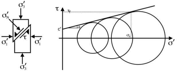
Figure 3: A graphical representation of the stresses on a sample and the representative Mohr’s Circle Diagram
However, in the case of clays that are loaded in the short term, pore water pressures are unable to immediately dissipate and therefore undrained conditions and a total stress analysis ensue. This also results in the friction angle being equal to zero which subsequently means that Mohr’s circles lie on a flat line friction line (Sivakugan, 2014).
3 Site Data
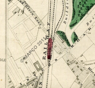
The site proposed for sampling has been chosen to be Finsbury Park Station (TQ 31332 86798) as borehole logs (Appendix 1) obtained from Network Rail records have indicated that it is likely that sampling from this site will provide samples of London Clay. Current works on the site include excavations and undercutting of the track to provide new disabled access to London Underground tube lines, therefore samples can be extracted from the core of the embankment therefore the site would be able to provide true representative samples from the core of the railway embankment, which have been remained in-situ since they were constructed around 170 years ago. It is also suitable that samples are collected from a main line into London because results from subsequent experiments will be attributable to the various main lines that travel into the capital, which is the main hub of transportation infrastructure and importance.
3.X Site History
Arkady (2013) explains that Finsbury Park Station was first constructed by navvies in the late 1840’s by the Great Northern Railway company. The site is situated in a low-lying area in comparison to the surrounding area and so the train line needed to be elevated between Holloway and Stroud Green to maintain sufficiently shallow track gradients. Therefore, an embankment was integrated into the construction design. The station was first introduced to connect the local populace and goods between Peterborough and Central London. Nowadays, Finsbury Park is used by over 28 million people annually and is a major transportation hub and interchange outside of Central London (Transport for London, 2015).
3.X Sample Collection and Storage
Soil specimens were excavated from Finsbury Park station on the 23rd December 2016 during routine excavation works that were being completed by the principal contractor, Spencer Group. It was previously arranged, through communication between the Author, Transport for London, Network Rail and Spencer Group, that ground personnel would dig out block samples from the core of the embankment, as the author was not permitted to undertake in-situ sample collection due to confined spaces permit restrictions. Post-collection measurements by the author rationalised that the block samples had been taken from approximately 3 metres below Moorgate Down Line rail level.
Soil specimens were taken as block samples; however, they were partially disturbed as they were not retained with their in-situ stresses in place. This resulted in the specimens being allowed to swell under atmospheric pressure conditions for for approximately six weeks. In addition, the author ensured the material was sealed in a polyurethane bag to ensure that the moisture content of the clay sample was relatively unchanged over this time period.
3.X Soil Classification Tests and Results
Succeeding soil collection, it is imperative that the soil is classified quantitatively to confirm its properties against the qualitative judgement that has been made. Soil classification was undertaken in accordance with BS 1377-2:1990, in which the plasticity index and material compositions were tested using Atterberg limits test, wet sieving and hydrometer test.
The Atterberg limits test was undertaken, using the cone penetrometer method (definitive method) for determination of the liquid limit. The liquid limit was determined, in accordance with BS 1377-2:1990, to be 58.3% and the plastic limit was determined to be 12.5%. These values result in a plasticity index of 46%.
Casagrande (1948), developed the plasticity chart, shown in Figure X, to determine the classification of the type of soil and the plasticity of the soil. The results show that this figure indicates that the soil is a high plasticity clay, which is representative of the classification given by Jones and Terrington (2011) who explain that London Clay formations become more plastic moving from West London to East London.
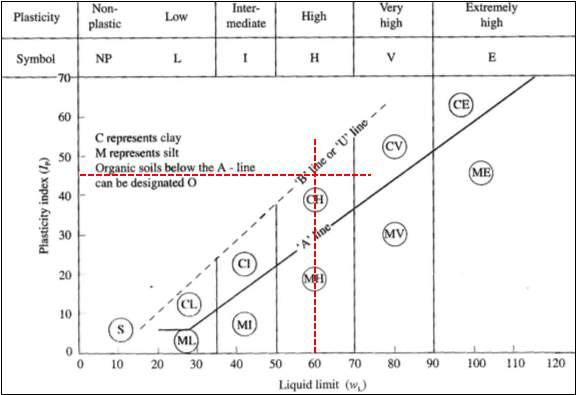
Figure 5: A graph using Liquid Limit and Plasticity to determine Soil Classification (Casagrande, 1948)
The author carried out a particle size distribution of a 500g sample to provide a representative indication of the material composition. Wet sieving was used to sort the soil sample into classes determined by particle size. These particle sizes were; 8.0mm, 4.0mm, 2.0mm, 1.0mm, 425µm, 250µm, 125µm and 63µm. A representative 50g sample of the material that passed through the 63µm was used to undertake a hydrometer test which determines, using Stokes Law, the relative densities of a liquid which changes as particles settle out of the suspension (Suryakanta, 2015). This in turn allows for the relative percentages of silts and clays within the sample to be determined.
The completion of a wet sieve and hydrometer test in accordance with BS 1377-2:1990 allows the formation of a particle size distribution graph, shown in Figure X.
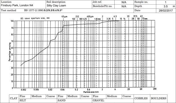
Figure 6: A graph to represent the Particle Size Distribution of sample collected from Finsbury Park Station
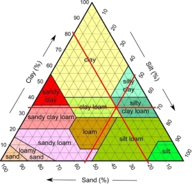
Figure X characterises the soil sample and shows that approximately 15% of the 500g sample consisted of sand and gravel particles, with the remaining 85% being made up of silts and clays. As shown in Figure X, this soil can be characterised dependent on the relative percentages of clay, sands and silts using the soil texture triangle, which ultimately classifies the soil as a silty clay loam/clay loam (USDA, 2017).
It is important that the soil, upon which the subsequent experiment will be based upon, is classified so that the results can be attributed to the properties of the London Clay Formation.
4 Methodology
After consideration of the research subject, literature review and sample specimens available, the author proceeded with an experimental approach to assess the effect of dynamic pore water pressure variations on samples of London Clay. For this, an experimental design will be needed.
4.X Triaxial Cell Test Overview
The triaxial cell test permits the control of confining pressures and internal pore water pressures on samples of soil. Additionally, the apparatus also allows for the control over whether tests are undertaken using drained or undrained conditions. The controls available using this test means that it will be able to facilitate the experiment that I will need to undertake although a few adjustments to the apparatus will need to be made.
The experiment will be split into five phases, which are:
- Reconstitution of the sample to provide homogenous specimens.
- Saturation of the sample to ensure that entrapped air is removed and pores are replaced with water.
- Consolidation of samples to 200kPa and dissipation of excess pore pressures.
- Cycling of pore pressures in the sample by ±50kPa
- Failure of samples to using deviatoric stress to assess ultimate failure strength.
However, there will be two sets of test specimens, where one specimen sample will go through Phases I to V whereas the other specimen sample will experience Phases I to III & V. This will allow a comparison to be made on whether the effect of cyclical pore water pressure have an effect on the ultimate failure strength of the clay soil.
4.X Experimental Procedure and Setup
4.X.X Specimen Reconstitution
It was foreseeable that the specimens that were collected from Finsbury Park would need to be reconstituted, as explain in section 3.X. This was due to the fact that there were sometimes large particles such as broken china and fragmented rocks that were in the sample that could have noticeably affected the ultimate failure strength of the specimen under triaxial conditions. A representation of their contribution to the overall sample composition can be seen in Figure X.
In order to reconstitute the sample in Phase I, a request was made to the Civil Engineering Mechanical Technician for a hydraulic setup with a 70mm bored steel tube that would allow a compressive force to be applied from the top to compress the sample down, shown in Figure X.
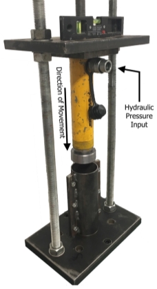
It is important that the soil is reconstituted in layers so that a consistent density of soil sample is formed within the mould. For a 140mm tall sample, it was decided to split this into 35mm increments which resulted in four layers of compaction. During the reconsolidation phase, the hydraulic jack input was set to the equivalent of 100kPa over three days which allowed the sample to consolidate and equilibrate pore pressures within the sample.
Another crucial step in the process was to ensure that once the specimen was removed from the reconsolidation apparatus, it was placed within the triaxial cell to prevent any swelling of the specimen, as it is exposed to atmospheric conditions, as this could result in the specimen reducing its degree of saturation as air is absorbed into the sample. This will subsequently prevent the moisture content of the sample being reduced.
4.X.X Triaxial Setup
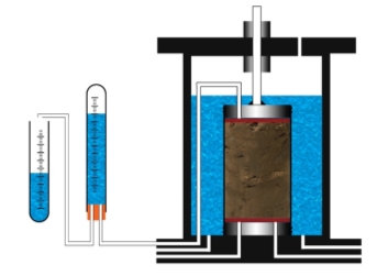
Following the undertaking of sample reconstitution in Phase I, the sample specimens were placed in the triaxial cell. However, as the sample needed to be saturated, the configuration of the apparatus needed to be changed as the pore pressure input for the cell was set up to be used with compressed air rather than compressed water, as laboratory experiments for undergraduates are undertaken using sand. This resulted in the addition of a secondary triaxial cell that was filled with water and connected to the primary triaxial cell through the pore water pressure input valve. Subsequently, this means that the pore pressure could be controlled in the primary triaxial cell through modification of the cell pressure in the secondary triaxial cell, as shown in Figure X.
Subsequently, the triaxial apparatus setup allows for Phase II to V to be undertaken. The features of the triaxial cell allow for the application of an isotropic confining stress (σ1), using cell pressures, and an anisotropic deviatoric stress (q), using a strain-controlled load frame, to produce a major principal stress (σ3), where:
[ 6 ]
q= σ3- σ1
The above applications of stress induce pressures on the outside of the sample’s membrane but it is also possible to control the pore pressures on the inside of the sample, which will subsequently alter the effective stress of the sample, as shown in Equation X.
Additional features of the triaxial cell are:
- Porous discs – These allow the drainage/even distribution of pore water pressures from the sample and also prevents the sample from blocking pressure lines coming from the top cap and bottom cap.
- Cell water – This is used to fill the cell on the outside of the membrane that that the majority of the void space becomes compressed water rather than compressed air. This is a safety precaution as water is less compressible than air.
- Vacuum line – This is to ensure that the sample is kept in place whilst the confining pressures within the triaxial cell are set up. The vacuum is also used, in this experimental setup, to allow excess pore pressures to drain from the sample. This will be explained in section X.X.
- Pressure gauges – These allow for transducers to be connected to the triaxial cell to measure the pressures within the cell and the sample.
- End caps – These permit the axial loading from the deviatoric load to be applied uniformly over the sample and ease the application of adding or withdraw pore pressures.
- O-rings – These affix the membrane to the end caps to prevent cell water from leaching into the sample.
- Force transducer – These measure the force applied by the deviatoric load piston in relation to its axial displacement.
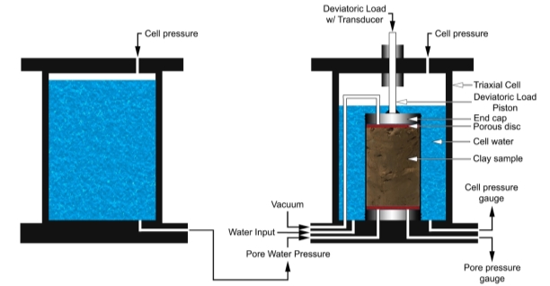
Figure 8: Diagram of Experimental Apparatus Setup
4.X.X Saturation
It is important to saturate the sample to ensure that any entrapped air is removed from the sample because the degree of saturation can influence the strength of a soil when placed in a triaxial cell. Yoshikawa et al (2015) explains that this is because air is highly compressible in comparison to water, which has a low compressibility and this subsequently affects the mechanical behaviour of the soil. Many tests have been undertaken to understand the behaviour of partially saturated soils but this is far less understood in comparison to the analysis of saturated soils.
Air has a density of 1.225 kg/m3 whereas water has a density of 1000kg/m3 therefore water is a lot denser than air and this understanding is important for the saturation procedure setup. During the interaction of air and water, their relative densities results in air wanting to rise and water wanting to sink. Therefore, during the saturation process, it is likely that when the entrapped air is removed from the sample, it is going to purge upwards towards the end cap. It is for this reason that the end cap will be open to atmospheric conditions to allow entrapped air to escape. This will be in addition to the pore water pressures that will purge through the sample from the bottom cap.
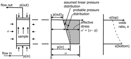
It was decided that the confining pressure of the specimen would be set to 100kPa as this is the pressure that the soil was subjected to in the reconstitution phase. However, 100kPa is larger than the pressure the soil was exposed when it was in-situ, as explained in section X.X.X. Therefore, any water purging from the sample through the vacuum outlet will be due to excess pore pressures as the top of the sample is consolidating, and also due to the differential pore water pressures throughout the sample, as shown in Figure X.
Figure 9: A diagram to represent the pore water pressure distribution within the sample and the associated effects on the effective stresses within the sample. Adopted from (Head, 2014)
4.X.X.X Skempton’s ‘B’ Pore Pressure Co-efficient
The calculation of Skempton’s ‘B’ co-efficient can determine the degree of saturation within a sample, where a sample can be regarded as ‘fully saturated’ when the degree of saturation is > 95% (Skempton, 1954). Barnes (2010) explains how Skempton’s coefficient is derived from the ratio of the average confining stress and the change in pore water pressure that is induced under undrained conditions, where:
B= 13(Δσ1+Δσ2+Δσ3)∆u
[ 7 ]
It is evident that in order to increase the average confining stress, the cell pressure of the triaxial cell will have to be increased and the subsequent change in pore water pressure measured. Consolidation of the specimens can be overlooked because this is occurring under undrained conditions as well as in the short term under isotropic conditions, therefore any pore water pressures will be hydrostatic as they will be unable to dissipate and shear is increased in all directions which will prevent the sample from failing in this mechanism.
Once the B coefficient has been calculated, this can be used to find the degree of saturation using Figure X, as shown below.
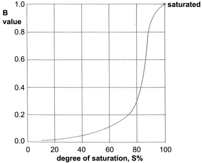
Figure 10: Relation between pore pressure coefficient, B and degree of saturation (%) (Barnes, 2010)
Full saturation of a sample is represented by a 95% degree of saturation, as explained above. Therefore, in relation to Figure X, a 95% degree of saturation is associated with a B coefficient of around 0.95. However, Rees (2013) states that the pore pressure coefficient is soil dependent, therefore full saturation may correspond to different B values given the type of soil. He also states that it may be possible for a stiff clay to exhibit full saturation at ~0.91.
4.X.X Consolidation
The consolidation stage of a clay soil is split into three phases, which are (Head and Epps, 2011):
- I: Initial compression
- This is due to the compression that is observed in pore spaces due to air and water and also the relaxing of the soil sample against the porous discs. This can also be attributed to instantaneous elastic strain induced in the sample.
- II: Primary consolidation
- This is due to the dissipation of excess pore pressures that have been induced from the increase in total stress. As these pore pressures dissipate, the effective stress of the soil is increased.
- Secondary consolidation
- Although excess pore water pressures have already dissipated, consolidation continues at a reduced rate as the movement of particles continues as the effective stress increases.
The experiment requires the consolidation of the soil specimens to similar pressures so that comparisons can be drawn between results. It was also decided to undertake an axis translations, which will be explained in section 4.X.X.X,because it is not known what conditions the London Clay samples have been subject to in the past, therefore the axis translation is used in order to ensure that all samples are translated into normally consolidated conditions. Consolidating the samples will also increase the density of the specimens which is advantageous as it ensures that the remoulded specimens are reconstituted well and will also provide a more obvious peak failure strength when this is tested after the consolidation phase. As part of the analysis of consolidation, the methodology will only assess the overall consolidation up to the end of the primary phase, as secondary consolidation analysis is beyond the scope of timescales available as part of this research dissertation.
4.X.X.X Axis Translation
An axis translation involves the increasing of confining pressures beyond what is initially needed and this allows the reduction of influences from soil suction properties in the soil. Figure X above denotes an axis translation where the Mohr’s circle on the right-hand side has higher confining stresses compared to the Mohr’s circle on the left-hand side; they have been translated along the X-axis.
Although saturation procedures will have been undertaken as part of the experimental procedure, it is unrealistic to guarantee that the samples become fully saturated due to the temporal limitations imposed. Vanapalli and Nicotera (2008) explain that partially-saturated samples result in a matric suction being induced in the sample because of the difference in pore air pressures and pore water pressures and axis translation helps to remove problems associated with cavitation within the soil specimen.
Furthermore, an axis translation will induce an increase in excess pore pressures within the sample and will constrict capillaries within the sample. This will result in pore liquids and pore gases being expelled from the soil samples and this will hopefully increase the saturation levels of the soil specimens. This is due to more air being drawn from the sample compared to water because air is less dense and will move out the sample more easily, especially as the pore pressures are released from the top of the soil specimen through the vacuum valve.
4.X.X.X Terzaghi’s 2D Consolidation Theory
Terzaghi (1943) explained the theory of consolidation as being “a decrease in water content of a saturated soil without replacement of the water by air is called consolidation”. For cohesive soils, the rate of consolidation for comparative settlement is slower because they exhibit a lower permeability in comparison to non-cohesive soils. For a soil specimen under vertically drained conditions, the rate of consolidation can be estimated through the following equation (Head, 2014):
Cv = 365TvH2t
[ 8 ]
Where:
- Cv = Coefficient of Compressibility (m2/year)
- Tv = Theoretical time factor
- H = Maximum drainage path length (metres)
- T = Consolidation time (days)
The theoretical time factor, Tv is calculated from its relationship with the degree of consolidation of the sample (%), where a Degree of Consolidation of 90% is represented as a dimensionless time factor of 0.848. The coefficient of consolidation can be calculated using the oedometer test, where load increments are loaded on a sample and its displacement is plotted against time. The gradient of this line is used to calculate the coefficient of consolidation, which can be used in the equation X.
Due to the time scales involved and availability of equipment, it was not possible for an oedometer test to be undertaken therefore an upper and lower limit have been taken from existing experiments, where London Clay has a lower limit coefficient of compressibility of 0.2m2/year and an upper limit of 2.0m2/year (Cripps and Taylor, 1986). These have been used to identify the upper and lower limits of the rate of consolidation for varying degrees of consolidation in Table X.
Table 2: A sensitivity table describing the minimum and maximum consolidation times for varying degrees of consolidation, Uv, for London Clay.
| Degree of consolidation, Uv (%) | Theoretical time factor, Tv | Drainage path length (m) | Minimum consolidation time, t (days) | Maximum consolidation time, t (days) |
| 10 | 0.0077 | 0.0700 | 0.00700 | 0.069 |
| 20 | 0.031 | 0.0700 | 0.0277 | 0.277 |
| 30 | 0.071 | 0.0700 | 0.0635 | 0.635 |
| 40 | 0.126 | 0.0700 | 0.113 | 1.13 |
| 50 | 0.196 | 0.0700 | 0.175 | 1.75 |
| 60 | 0.286 | 0.0700 | 0.256 | 2.56 |
| 70 | 0.403 | 0.0700 | 0.360 | 3.60 |
| 80 | 0.567 | 0.0700 | 0.507 | 5.07 |
| 90 | 0.848 | 0.0700 | 0.758 | 7.58 |
| 95 | 1.129 | 0.0700 | 1.01 | 10.1 |
| 100 | ∞ | 0.0700 | ∞ | ∞ |
For the experimental procedure, I will be using the upper limit of the 90% degree of consolidation, which is 7.58 days, to leave the sample to consolidate for after it has been saturated. After the consolidation phase has been completed, one specimens will subsequently go through phase IV and V whilst the other specimen will go straight to phase V for the ultimate failure strength test.
4.X.X Pore Pressure Cycles
The scope of this research dissertation looks at how the effect of dynamic pore water pressures affect the ultimate failure strength of the soil sample. The author has determined three different possible methods that can be used to cycle the pore water pressures within the sample.
The first method looks at increasing the cell pressure under undrained conditions which would result in the increase in hydrostatic pore water pressures within the specimen. This method is advantageous because is it quick and pore water pressures are induced from instantaneous excess pore pressures within the sample. However, these pore water pressures are induced due to the skeleton of the soil sample wanting to consolidate, so this principle is primarily conforming to Newton’s Third Law. Furthermore, the increase in confining stresses are proportionately matched by the increase in excess pore pressures, therefore the effective stresses of the sample are unchanged, as shown in the following equation:
[ 9 ]
σ’=σ+∆σ – [u+∆σ]
The second method looks at controlling pore water pressures from the end caps of the sample and regulating the change in pore pressure using a backup triaxial water chamber, as shown in Figure X above. However, changes in the pore pressures over the long term would subsequently affect the effective stresses within the sample, which will result in the specimen consolidating or swelling, dependent on whether the applied pore water pressures are positive or negative of their equilibrium value. Therefore, in order to prevent the change in mechanical behaviour occurring due to consolidation, as the pore water pressures are increased, the confining stresses can also be increased to ensure that the effective stresses within the sample are unchanged.
The third method looks at releasing some of the cell pressure under drained conditions which results in the decrease in internal pore water pressures in the short term which results in suction effects as the sample wants to draw water back in to reacquire equilibrium. Once this stage has been completed, the sample will be reconsolidated causing an increase in pore water pressure which will dissipate with time. By reducing the cell pressure of the sample and going reconsolidating to its previous state, this will prevent the sample from being in an over consolidated state in comparison to Specimen A.
The second method has the potential to be the best at understanding whether dynamic pore water pressures have an effect on the ultimate failure strength as the sample will be unable to consolidate as effective stresses are controlled and any changes in mechanical behaviour can be attributed to changes in internal pore pressure. However, the timescales that will be required to undertake this methodology are beyond the scope of this this research project. It would also prove a difficult methodology to manage because cell and pore pressures would have to be increased incrementally every hour for innumerable days as it would be important not to induce excess pore pressures that would ultimately change the effective stress if the pore pressure control is also being increased incrementally.
Therefore, the dynamic pore water pressures will be controlled using the third method and the loading path of this method can be seen in Figure X.
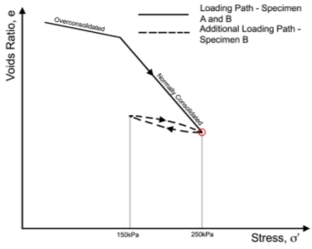
Figure 11: A graph to represent the loading paths of specimen’s A and B. Adopted from (Figure X.X; Barnes, 2010)
4.X.X Consolidated-Drained (CU) Triaxial Compression Test
Following phase I to III for Specimen A and phase I to IV for Specimen B, the ultimate failure strength of each specimen needs to be tested using the triaxial cell. As shown in Figure X, the deviatoric load piston is attached to a strain rate loading frame, which subsequently applies a deviatoric stress, q, to the sample. The test will occur under CU (Consolidated-Undrained) conditions; therefore, the drainage valves will be closed and pore pressures will be unable to dissipate. It is not possible to undertake a CD (Consolidated-Drained) due to the time limitation of the research project and the strain loading frame has a pre-set of one value of strain rate which cannot be altered. It would still be possible to undertake but would require constant supervision to incrementally fail the samples.
During the experiment, the following parameters will be recorded (British Standards, 1990; McAfee, 2007):
- Time – This is required so that all following parameters can be attributed to the same period in time for comparison.
- Cell Pressure – Will be kept constant from compressed air inlet but changes within the triaxial cell as the sample deforms could cause fluctuations in the cell pressure.
- Pore pressure – this will allow us to determine the excess pore pressures that are building up within the sample as the soil skeleton wants to decrease in volume.
- Load – this is recorded through a transducer in the deviatoric load piston and allows a relationship between load and strain to be made.
- Displacement – this will allow the strain of the sample to be calculated and determine the relationship with the load (mm).
These parameters will then be used to produce a graphical analysis of the failure criterions, as shown in the next section.
5 Results
All results and data applicable to reconstitution, moisture content, saturation, consolidation and triaxial compression tests have been incorporated into the USB drive submitted as part of this research dissertation. (Note: this drive can be found on the back cover of this research dissertation).
5.X Saturation
After the reconsolidation of Specimen A and Specimen B under a pressure of 100kPa in the reconsolidation rig, a quantitative estimation of saturation was interpreted using Skempton’s Pore Water Pressure Coefficient, as explained in section X.X. The results of these are tabulated in Table X below.
Table 3: A table showing the data attributed to Skempton’s Saturation B-Check for Specimen A and Specimen B
|
Specimen |
InitialPore Pressure (kPa) |
Final Pore Pressure (kPa) |
Pore Pressure Difference (kPa) |
Initial Cell Pressure (kPa) |
Final Cell Pressure (kPa) |
Cell Pressure Difference |
B-Value |
Saturation (%) |
| A | 100.3 | 139.0 | 38.7 | 101.7 | 151.0 | 49.3 | 0.80 | 87 |
| B | 99.9 | 139.6 | 39.7 | 103.1 | 151.8 | 48.7 | 0.82 | 89 |
Ultimately, both specimens exhibited similar degrees of saturation but both were notably below the 95% level upon which a sample can be considered as being fully saturated. Therefore, it can be said that although both specimens were near to full saturation, they were in fact partially-saturated samples.
5.X Consolidated-Drained (CU) Triaxial Compression Test
5.X.X Graphs
In accordance with BS1377-8 and McAfee (2007), values for parameters described in section 4.X.X were recorded during the triaxial test and logged into an ancillary excel spreadsheet. These values allow a graphical representation to be made to determine the failure strength of the soil as well as the soil’s previous condition from the behaviour the sample expresses during the compression test. A comparative graphical representation of Specimen A and Specimen B can be seen in Figure X, Figure X and Figure X below.
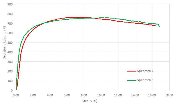
Figure 12: A graph to show the comparison between the relationship of deviatoric load (q) and strain (%) for Specimen A and Specimen B
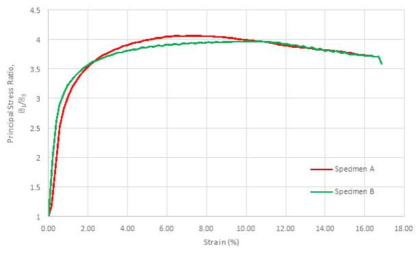
Figure 13: A graph to show the comparison between the relationship of Principal Stress Ratio ( 1/ 3) and Strain (%) for Specimen A and Specimen B
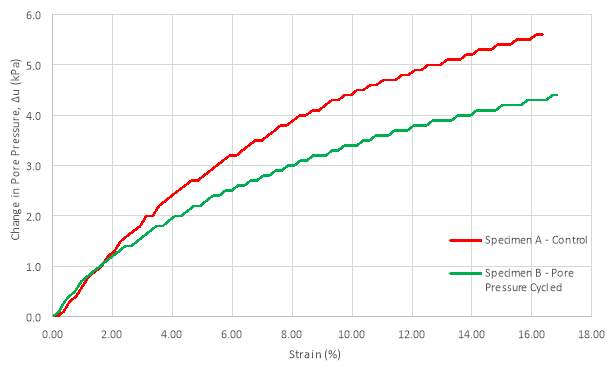
Figure 14: A graph to show the comparison between the relationship of Change in Pore Pressure (∆u) and Strain (%) for Specimen A and B
5.X.X Mohr’s Circle Theorem
Mohr-Coulomb theorem, as described in Section X.X has been used to generate the Mohr’s circle for Specimen A and Specimen B, as shown in Figure X and Figure X. These represent the major and minor principal stresses as well as the maximum shear forces and failure mechanism.
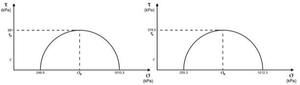
Figure 15: Two Mohr’s Circle Diagrams for Specimen A (left) and Specimen B (right)
5.X.X Post Test Pictures
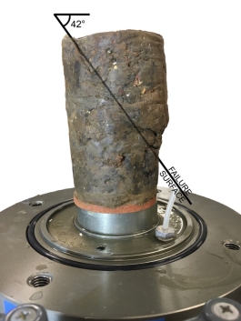
Figure X shows Specimen A after the compression test has taken place whilst Figure X shows Specimen B after the compression test has taken place. Both figures clearly exhibit a failure surface, as depicted in the picture with the lines of intersection.
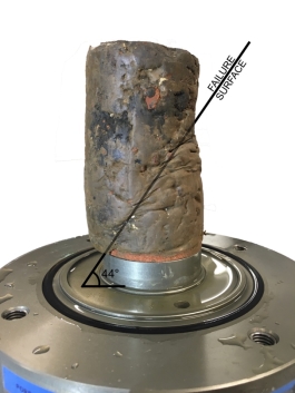

Figure 16: A picture of Specimen A Post-Triaxial Compression Test. Shear failure plane can be clearly seen.
Figure 17: A picture of Specimen B Post-Triaxial Compression Test. Shear failure plane can be clearly seen.
6 Discussion
The purpose of this research dissertation was to design and develop an experimental procedure to investigate the effect of cyclical pore water pressure variations on the deterioration of soil strength of Finsbury Park Station earthworks. This experimental procedure was then used to test two reconstituted London Clay samples from the core of the railway embankment to help evaluate the experimental procedure and determine, from test results, whether an effect on soil strength could be seen due to the cyclical nature of pore water pressures on the samples.
It is important to note that due to the constraints posed by the temporal limitations of the research dissertation and the complexity of the experimental procedure, it was not possible to test the number of samples that would be required to draw a conclusive evaluation of the effect of pore pressure cycles on the failure strength of the samples.
6.X Visual Analysis
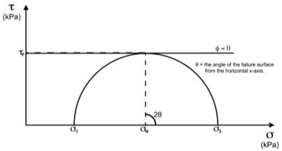
Figure X and Figure X present the failure surfaces of Specimen A and Specimen B, respectively, after the samples had been subject to the triaxial compression test. Using a clinometer, the failure angle of both specimens was shown to be around 45˚. Specimen A had a failure angle of 44˚, whilst Specimen B had a failure angle of 42 degrees. The close proximity to a 45˚ failure plane proves that the triaxial test was undertaken under undrained conditions because a 45˚failure angle (θ) denotes a phi (ϕ) angle equal to zero, as shown in Figure X below.
Figure 18:A representation of the angle of the failure surface in relationship to the Mohr’s Circle and associated phi angle. Adopted from (Helwany, 2007)
The line dotted line drawn from the normal failure stress on the x-axis that intersects the maximum shear force at the edge of the circle is perpendicular to the line that denotes the angle of friction, where, in this case:
[ 10 ]
θ= 90- ϕ2=90-02=45°
The fact that both angles of failure are slightly lower than 45 degrees would mean that a slightly lower shear stress and normal stress would have resulted in the failure plane. Subsequent analyses will consider the total stress conditions to be undrained with a phi angle equal to zero, representing a homogenous failure plane angle of 45 degrees across Specimen A and Specimen B.
6.X Graphical Analysis
6.X.X Peak Failure Strength,
τFThe relationship between the deviatoric load and the strain of each sample can be seen in Figure X. These relationships show a region of linear elastic deformation for the first 1% of strain for both specimens. As the soil is mobilised beyond this 1% strain, as shown in Figure X, the increase in strain is no longer proportional to the increase in stress. The gradient of the line decreases until the material exhibits a peak failure strength at the point where, generally:
[ 10 ]
dqdε→ 0 or dqdε=0
The results show that where the above Equation X holds, Specimen A exhibits a peak deviatoric strength of 762kN/m2 whilst Specimen B exhibits a peak deviatoric strength of 757kN/m2. Once Equation X has tended towards and surpassed zero, there is a subsequent plateauing of deviatoric load with increasing strain with a slight decrease in deviatoric stress as strain increases. This slight decrease could be representative of the density of the sample as the soil wants to shear but not all parts of the failure surface are able to shear at the same time and the soil particles need to move upwards as well as laterally to overcome the friction between soil particles (Heath, 2014).
A significant peak on this figure would represent the behaviour of an over consolidated clay, as shown in Figure X, but the small significance of the peak shown in Figure XX leads the author to believe that the clay has been normally consolidated and therefore was recognised to have an Over-Consolidation Ratio (OCR) of 1.0 prior to testing but post-consolidation phase. There are two further checks that can be used to determine that the clay samples were normally consolidated, which are:
- Sample Collection
- The samples taken from Finsbury Park Station were taken from an approximate depth below the railway track of 3.00m which would represent a compressive vertical force of 60kPa. However, this soil would have been originally taken from a cutting but no cuttings in the surrounding vicinity of Finsbury Park station exhibit cuttings that are more than 8m deep. Therefore, the consolidation of the specimens to 250kPa can be deemed more than adequate the ensure that the OCR of the specimens is 1.00, where:
[ 11 ]
OCR= Maximum Stress in HistoryCurrent Effective Stress
- Pore Pressure Behaviour
- An indication of the previous stress history of a soil sample can be made by analysing the behaviour of the pore pressure gauge as a soil sample is failed in the triaxial compression test. These behaviours can be seen in Figure X below.
The normally consolidated sample illustrates a logarithmic curve of increasing pore pressure as the volume of the sample wants to change by dissipating excess pore pressures to allow the consolidation of the sample through compression of the soil skeleton. This behaviour is reflected in the Figure X for both samples. This is in comparison to over consolidated behaviour where suction pressures are induced in the sample because, as the sample is sheared, the sample expands to overcome the frictional forces of the soil particles on either side of the failure plane.
- An indication of the previous stress history of a soil sample can be made by analysing the behaviour of the pore pressure gauge as a soil sample is failed in the triaxial compression test. These behaviours can be seen in Figure X below.
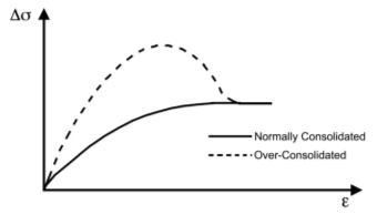
Figure 18: A diagram to represent the behaviours of normally consolidated and over-consolidated soils on the relationship between deviatoric stress and strain. Adopted from Barnes (2010)
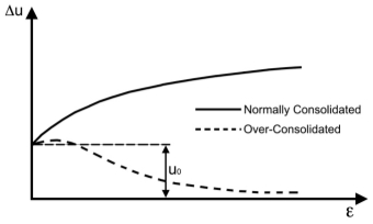
Figure 19: A diagram to represent the change in pore pressure with increasing strain for normally consolidated and over consolidated samples.
These checks have given a good indication that both samples have been normally consolidated which confirms the homogenous behaviour of the two samples. This subsequently endorses the validity of further comparisons.
6.X.X Modulus of Elasticity
Another indication of the effects of cyclical pore water pressure variations on the mechanical composition of the clay soil samples would be the change in stiffness of the materials. It has been noted that the stiffness of a soil sample cannot simply be attributed to gradient of the linear relationship of the stress-strain curve as it is for standard materials. It is in fact much more complex in soil geotechnics (Briaud, 2001) .
The complexity lies in the fact that the Poisson’s ratio (υ) of the soil is unknown and the soil is under confining stresses when in the triaxial set up. It is useful to note that the stiffness can be an indicator of the effect of dynamic pore water pressures, however, due to it its complexities and deviation from the scope of this investigation, it will not be discussed further.
6.X Experimental Procedure Analysis and Evaluation
This section will focus particularly on the evaluation of the design of the laboratory experiment in acquiring the data displayed in section X.X. It will also look at ways in which the experimental process could be improved and how experimental techniques could be improved should the experiment be repeated.
6.X.X Phase X – Reconstitution
The reconstitution stage was very effective in producing two homogenous specimens, the construction of which was described in section X.X. It was important that the specimens were compacted in layers so that there would be a consistency of density throughout the length of the sample. Both specimens were compacted in 4 layers of around 40mm layer to get a total height of 160mm, where the excess would be trimmed off are the reconstitution phase to get two specimens both 140mm in height.
6.X.X Phase X – Saturation
The saturation phase of the experiment proved difficult to undertake due to various factors. The system setup looked at increasing the pore water pressure at the bottom cap of the triaxial sample whilst leaving the top cap open to atmospheric conditions. The idea of differential pressures at either end was decided to induce a pressure gradient across the sample, in order to coax water into flowing through the sample to remove the entrapped air, as described in section X.X and Figure X. However, in retrospect, this may not have been the best procedure to undertake as this differential pressure gradient resulted in the confining pressures across the specimen to cause differential consolidation of the sample due to the difference in effective stress. Although the effects of this would have been considerably reduced in the consolidation phase, this may have altered the mechanical behaviour within the sample. On the other hand, it was necessary to ensure that the top cap was open to atmospheric conditions so that air could escape from the sample and transition the specimen from a partially saturated to a fully saturated sample. Alterations to the setup could have been made to enable the escape of air whilst maintaining a back pressure on the top cap but due to the time constraints and equipment available, exploration of this possibility did not occur.
Furthermore, it was essential to maintain similar cell and back pore pressures, with the cell pressure being slightly higher (3kPa) than the pore pressure, to ensure that the pore pressure didn’t cause the sample membrane to swell into the triaxial void. The idea of similar pressures was used to ensure that capillaries within the sample did not close and prevent the movement of water through the sample.
Additionally, determination of the degree of saturation, as described in section X.X, was made using Skempton’s B-Check procedure. The initial success of this procedure was good during the saturation phase of the experiment however during the consolidation phase, the B-check calculation became irregular and no longer followed a pattern, therefore the degree of saturation of the specimen after consolidation could not be calculated. This could have been attributed to the fact that during the consolidation phase, both ends of the sample were subject to atmospheric conditions. Therefore, when the drainage valves are closed, as shown in Figure X, there is no back-pore pressure locked in the short length of pipe between the bottom cap and the drainage valve, therefore larger pressures would be needed to induce the change in pore pressure value needed in Equation X. This is the reason that additional pore pressure were applied at the end caps before the triaxial compression test but this will be discussed in section X.X
Time limitations to the experimental procedure resulted in the saturation phase having to be cut short of the full saturation percentage of 95%. Specimen A and Specimen B had respective values of 87% and 89% degrees of saturation which would means that some of the voids within the sample are occupied by air rather than water, which is preferable. The presence of a combination of air and water within voids has an effect on the shear strength in clays because air is more compressible than water and therefore the pore water pressures will increase at a faster rate in comparison to pore air pressures when a triaxial sample is subject to loading (Kamata et al, 2009).
Additional improvements to the saturation phase of the experiment would have been to incorporate a dual pipette method that would have enabled periodical measurements of air and water escaping from the top cap of the triaxial cell, as shown in Figure X below. A graph of these volume changes against time would have reinforced the results of Skempton’s B-Check by visualising the plateauing of cumulative air volume escaping from the specimen.
6.X.X Phase X – Consolidation and Unloading
The consolidation phase of the experiment was relatively straight forward and followed the loading path, as shown in Figure X, which denotes the change in voids ratio with increasing isotropic confining stress. Both specimens were subject to the same consolidation time, which was calculated using Terzaghi’s consolidation theorem, which is explained, in detail, in section X.X. The accuracy of the extent of consolidation could have been improved through the use of volume change units, which were unfortunately unavailable for use during the experimental period. The integration of volume change units would have made the degree of consolidation easier to visualise. Consolidation follows a curve which tends towards the finite end specimen height, at the time period of infinity. Therefore, the rate of consolidation will decrease with time as the same moves from primary to secondary compression. A graph representing change in volume (∆V) against time (t) would have allowed the consolidation phase to be stopped when the rate of change of volume was below a certain value. Another method that could have been employed would have been through having a pore pressure applied at both the top and bottom end cap. Once the pore water pressures had equalised to the readings taken previous to the consolidation procedure, consolidation could be deemed as complete because all the excess pore pressures have made their way out the sample.
Further to the consolidation phase was the unloading phase, which was only relevant to Specimen B as Specimen A was the control specimen. This involved reducing the confining stresses, as described in section X.X. This reduction in confining pressures would have resulted in the swelling of the clay sample which encompasses the expansion of the soil skeleton. This in turn induces a change in pore water void pressure which is below that exerted on the water by the skeleton which results in suction pressures within the voids and water is drawn back into the specimen. It was noted at the end of the consolidation phase that there was still air trapped within the vacuum tube, therefore some of this air would have unfortunately re-entered the sample and subsequently altered the degree of saturation. Nonetheless, it is likely that the air would have exited the sample when the confining stresses were reapplied to the specimen.
6.X.X Phase X – Triaxial Compression
It was through this phase of the experiment that the results due to the effect of changes in pore pressure on the strength of the soil would be obtained. Preceding the start of this phase, the author realised that the effect of consolidation under atmospheric pore pressure conditions had resulted in a delayed response to changes in pore pressure when additional confining stresses were added to the sample under undrained conditions. Therefore, the author decided to apply a back-pore pressure of 10kPa to either ends of the specimen in the hope that changes to pore pressure (∆u) could seen more clearly. It is important to note that this application of back-pore pressure was applied 5 minutes before the start of the compression phase therefore it should not have altered the internal pore pressures within the sample. The subsequent changes in pore pressure through application of deviatoric load can be seen in Figure X.
6.X Future Experimental Amendments
The majority of amendments that the author would make to the experimental procedure were due to the time constraints imposed by the project. With more time, the first step would have been to ensure that both specimens were saturated to at least 95%, which would have been possible if the specimens were saturated for one week longer.
Secondly, the addition of volume change units would have provided a graphical interpretation of the specimens transitioning from primary to secondary consolidation and the consolidation of both specimens could have been stopped when the strain rate reached a set value. This would have enabled homogenous consolidation exposure and settlement to each specimen and improved the validity of further comparison in the superseding phases of the experimental procedure.
Thirdly, it was noted that the use of tap water in the back-pore pressure saturation phase resulted in dissolved air being introduced to the specimen. This can subsequently lead to false reading on the pore water pressure gauge (Been and Jeffries, 1985). Therefore, the author is suggesting the addition of a de-aired water system which agitates the water and causes cavitation and nucleation to occur which subsequently expels any dissolved gases from the liquid (Been and Jeffries, 1985).
A penultimate consideration would be to extract block samples from the ground instead of cuttings which had to be reconstituted. Block samples or core samples would prevent the disturbance of the sample and provide a sample that is representative of the ground conditions and constitution that it was when in the ground.
Finally, the author should have previously considered the removal of air from the line between the bottom porous disc and the pore water pressure valve and the line between the top porous disc and the vacuum valve. Removal of this air would have made it easier for the water to move through the sample and it would have also improved the readings on the pore water pressure gauge that was attached to the bottom cap of the sample.
7 Conclusion
Ultimately, due to the time constraints of the research dissertation and the limit of equipment availability, this research dissertation will not be able to draw any conclusive evaluations on the effect of dynamic pore water pressure variations on the soil strength of the specimens. However, an evaluation of the design of the experimental procedure has been made as well as an analysis of the results so that a hypothetical conclusion can be made.
In terms of the aims and objectives of this research dissertation, as discussed in section X.X, this research dissertation was undertaken to investigate the effect of cyclical pore water pressure loading variations on samples of London Clay, using a triaxial test, under CU conditions. The five objectives set in section X.X were instigated in order to reach this aim. The success and usefulness of these objectives in relations to the overall aim were largely similar except from objective IV, where the objective looked at undertaking a CU test on a cut sample of London Clay so that a control failure strength could be determined. Through the course of the experiment, the relevance of this test diminished because the comparison between this control value and the subsequent failure strengths would not have been able to be made because of the differential preparation of the specimens. It was previously decided that this control sample would be cut from a block and be largely undisturbed in comparison to the other specimens. Subsequently, literature brought to light that the difference in behaviour between cut and reconstituted samples would vary greatly and so it would be impossible for comparisons to be made. Therefore, the it was decided that the control specimen and the specimens that was to be effected by the dynamic pore water pressure variations would be both made from reconstituted samples.
The design of the experimental procedure was suitable for the investigation of the dissertation aim and definite conclusions would have been made if more samples were tested. If the experiment was to continue, the author would have tested three control samples and a mean control failure strength would have been determined. This would have been followed by nine subsequent samples with three varying numbers of dynamic cycling. This would allow not only the effect of dynamic pore water pressures on the failure strength to be investigated but also the extent to which these dynamic cycles can affect the failure strength.
Having completed the experimental procedure, the author determined a number of key considerations and improvements that could be made to the experiment. These included the improvement of the saturation procedure through the addition of the saturation of cables attached to the sample before the saturation procedure commenced, as well as ensuring that the specimens were saturated to at least 95% using de-aired water. Additional major considerations would have been the addition of volume change units to the triaxial cell as these would have supported the quantitative progression through the consolidation and unloading phase. And lastly, the sampling technique of using block or core samples so that samples are not disturbed and the reconstitution phase of the experiment is not needed.
8 References
American Association of State Highway and Transportation Officials (AASHTO), 2008. Guide Specifications for Highway Construction. Washington, DC.
Arkady, 2013. The Past and Future of Finsbury Park – London Reconnections [Online]. Available from: http://www.londonreconnections.com/2013/the-past-and-future-of-finsbury-park/ [Accessed 21 February 2017].
Barnes, G., 2010. Soil Mechanics: Principles and Practice. 3rd ed. New York, NY, USA: Palgrave Macmillan.
BBC News, 2015. Toilet Waste Horrors on UK Train Tracks [Online]. Available from: http://www.bbc.co.uk/news/uk-england-30541015 [Accessed 2 January 2017].
Been, K. and Jefferies, M.G., 1985. A state parameter for sands. Géotechnique, 35(2), pp.99–112.
Biondi, G., Di Filippo, G., and Maugeri, M., 2007. Effect of Earthquake Induced Pore-Water Pressure in Clay Slopes. In: 4th International Conference on Earthquake Geotechnical Engineering. Thessaloniki, Greece: 4ICEGE, pp.1–12.
Bobet, A., 2003. Effect of pore water pressure on tunnel support during static and seismic loading. Tunnelling and Underground Space Technology, 18(4), pp.377–393.
Boussinesq, V.J., 1885. Application des potentiels a l’etude de l’equilibre et du movement des solides elastiques. Paris, France.
Briaud, J. L., 2001. Introduction to Soil Moduli. Texas, USA.
Briggs, K.M., Loveridge, F.A., and Glendinning, S., 2016. Failures in transport infrastructure embankments. Engineering Geology, 219(1), pp.1–11.
British Standards Institution, 1990. Soils for Civil Engineering Purposes – Part 8 (Effective Shear Tests). London, UK.
Brooker, E.W. and Ireland, H.O., 1965. Earth Pressures at Rest Related to Stress History. Canadian Geotechnical Journal, 2(1), pp.1–15.
Casagrande, A., 1948. Classification and Identification of Soils. Transaction of the American Society for Civil Engineers, 113(1), pp.901–930.
Charlafti, M., 2014. Slope Stability and Vegetation [Online]. Journal of Architectural Engineering Technology, 3(4), pp.4–11. Available from: http://www.omicsgroup.org/journals/architectural-engineering-technology-abstract.php?abstract_id=42556.
Cripps, J.C. and Taylor, R.K., 1986. Engineering Characteritics of British Overconsolidated Clays and Mudrocks. Engineering Geology, 22(1), pp.349–376.
Endo, T., 1980. Effect of Tree Roots upon the Shear Strength of soil. Forest and Forestry Products Research Institute, 14(2), pp.112–115.
Esveld, C., 2001. Modern Railway Track. 2nd ed. Zaitbommel, Netherlands. Available from: http://www.esveld.com/MRT_Selection.pdf.
Graham, J., Noonan, M.L., and Lew, K. V., 1983. Yield states and stress–strain relationships in a natural plastic clay [Online]. Canadian Geotechnical Journal, 20(3), pp.502–516. Available from: http://www.nrcresearchpress.com/doi/abs/10.1139/t83-058#.UrO1yBuVN6I%5Cnhttp://www.nrcresearchpress.com/doi/abs/10.1139/t84-064#.UrO1iBuVN6I.
Greater London Authority, 2011. Assessment Drain London London Borough of Islington. London, UK.
Head, K.H. and Epps, R.J., 2011. Manual of Soils Laboratory Testing. 3rd Editio. Whittles Publishing.
Head, K.H. and Epps, R.J., 2014. Manual of Soil Laboratory Testing – Volume III: Effective Stress Tests. 3rd Editio. London, UK: Whittles Publishing.
Heath, A., 2015. Soil Mechanics Shear Strength Lecture. , p.5.
Helwany, S., 2007. Shear Strength of Soil [Online]. Applied Soil Mechanics: with ABAQUS Applications, pp.162–208. Available from: http://onlinelibrary.wiley.com/doi/10.1002/9780470168097.ch5/summary.
Heyman, J., 1972. Coulomb’s memoir on statics: An essay in the histroy of civil engineering. Cambridge, UK: Cambridge University Press.
Ishak, M.F., Ali, N., and Kassim, a., 2013. The Influence of Tree Induced Suction on Soil Suction Profiles. International Journal of Research in Engineering and Technology, 2(9), pp.187–193.
Jones, L.D.D. and Terrington, R., 2011. Modelling Volume Change Potential in the London Clay [Online]. Quarterly Journal of Engineering Geology and Hydrogeology, 44(1), pp.109–122. Available from: http://qjegh.lyellcollection.org/cgi/doi/10.1144/1470-9236/08-112%5Cnhttp://qjegh.geoscienceworld.org/content/vol44/issue1/.
Kamata, T., Tsukamoto, Y., and Ishihara, K., 2009. Undrained Shear Strength of Partially Saturated Sand in Triaxial Tests B =. Bulletin of the New Zealand Society for Earthquake Engineering, 42(1), pp.57–62.
Labuz, J.F. and Zang, A., 2012. Mohr-Coulomb Failure Criterion. Rock Mechanics and Rock Engineering, 45(6), pp.975–979.
Lamri, I. and Hidjeb, M., 2008. Pore Pressure and Strength Behaviour of Clay Under Cyclic Loading . Proceedings of the 4th WSEAS International Conference on applied and theoretical mechanics (Mechanics 2008), pp.44–51.
Lee, K. and Focht, J.A., 1975. Strength of Clay subjected to cyclic loading. Marine Geotechnology, 1(3).
Lucas, J., 2012. Damaged Vale of Rheidol Railway Embankment [Online]. Available from: http://www.geograph.org.uk/photo/2991261.
Manolopoulou, A., 2009. The Industrial Revolution and the changing face of Britain [Online]. Available from: http://www.britishmuseum.org/research/publications/online_research_catalogues/paper_money/paper_money_of_england__wales/the_industrial_revolution.aspx [Accessed 24 April 2017].
McAffee, R.P., 2007. Laboratory Tests to Determine Shear Strength of Soils. Geotechnical Engineering II.
Mitchell, J.K., 1960. Components of Pore Water Pressure and Their Engineering Significance. Clays and Clay Minerals, 9(1), pp.162–184.
Mohr, O., 1900. Welche Umstånde bedingen die Elastizitåtsgrenze und den Bruch eines Materials? Zeit des Ver Deut, 44, pp.1524–1530.
Mott MacDonald, 2011. The Effects of Railway Traffic Loading on Embankment Stability.
Norwest Holst, 2007. Finsbury Park Station Ground Investigation. London, UK.
Nowak, P. and Gilbert, P., 2015. Earthworks : a Guide. London, UK: Institution of Civil Engineers.
O’Brien, A.S., Briggs, K.M., Smethurst, J. a., and Powrie, W., 2013. Wet winter pore pressures in railway embankments [Online]. Proceedings of the ICE – Geotechnical Engineering, 166(5), pp.451–465. Available from: http://www.icevirtuallibrary.com/content/article/10.1680/geng.11.00106.
Perry, J., 2003. Infrastructure cuttings condition appraisal and. , pp.174–180.
Perry, J., Pedley, M., and Reid, M., 2001. Infrastructure embankments: Condition Appraisal and Remedial Treatment. CIRIA Report C550, pp.174–180.
Ramiah, B.K., Dayalu, N.K., and Purushothamaraj, P., 1970. Influence of Chemicals on Residual Strength of Silty Clay. University College of Engineering, Bangalore, India.
Rees, S., 2013. Introduction to Triaxial Testing [Online]. Available from: http://www.gdsinstruments.com/__assets__/pagepdf/000037/part 1 of 3_.pdf.
Rushton, K.R. and Ghataora, G., 2012. Design for efficient drainage of railway track foundations. Proceedings of the ICE – Transport, 167, pp.1–12.
Seed, H.B. and Martin, G.R., 1966. The Seismic Coefficient in Earth Dam Design [Online]. American Society of Civil Engineers, 92(SM3), pp.25–58. Available from: https://trid.trb.org/view.aspx?id=38521.
Selig, E.T. and Sluz, A., 1978. Ballast and Subgrade Response to Train Loads.
Sivakugan, S., 2014. Drained vs Undrained Loadings in Geotechnical Engineering [Online]. Available from: https://www.linkedin.com/pulse/20140618014822-6961529-drained-vs-undrained-loadings-in-geotechnical-engineering.
Skempton, A.W., 1996. Embankments and Cuttings on the early Railways. Construction History, Vol. 11, pp.33–49.
Skempton, A.W., 1954. The Pore-Pressure Co-efficients A and B. Imperial College, London.
Stanford, E., 1872. Stanfords Library Map of London and Suburbs [Online]. Available from: http://london1872.com/stanford21.htm.
Suryakanta, 2015. Hydrometer Analysis of Soil – What, Why and How? [Online]. Available from: http://civilblog.org/2015/11/18/hydrometer-analysis-of-soil-what-why-how/#.
Terzaghi, K., 1925. Erdbaumechanik auf bodenphysikalischer grundlage. University of California.
Terzaghi, K. von, 1943. No Title. In: Theoretical Soil Mechanics. Hoboken, NJ, USA: John Wiley and Sons Inc. Available from: http://onlinelibrary.wiley.com/doi/10.1002/9780470172766.ch13/summary.
Tranport for London, 2015. Multi-year station entry and exit figures. , p.1.
USDA, 2017. Soil Texture Calculator [Online]. Available from: https://www.nrcs.usda.gov/wps/portal/nrcs/detail/soils/survey/?cid=nrcs142p2_054167.
Vanapalli, S.K. and Nicotera, M.V., 2008. Axis Translation and Negative Water olumn Techniques for Suction Control. Geotech Geol Eng, 26(1), pp.645–660.
Yoo, T.S. and Selig, E.T., 1979. Field Observations of Ballast and Subgrade Deformations in Track.
Yoshikawa, T., Noda, T., and Kodaka, T., 2015. Effects of air coupling on triaxial shearing behavior of unsaturated silty specimens under constant confining pressure and various drained and exhausted conditions [Online]. Soils and Foundations, 55(6), pp.1372–1387. Available from: http://dx.doi.org/10.1016/j.sandf.2015.10.004.
9 Appendix A – Borehole Log Information – Finsbury Park Station P8 (Norwest, 2007)
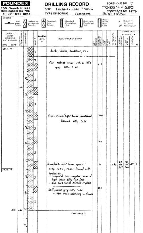
Cite This Work
To export a reference to this article please select a referencing stye below:
Related Services
View all


Related Content
All TagsContent relating to: "Ecology"
Ecology is a field of biology that concentrates on the study of the relationships and interactions between living organisms (including humans) and their environments.
Related Articles

DMCA / Removal Request
If you are the original writer of this dissertation and no longer wish to have your work published on the UKDiss.com website then please: