Abstract

In present scenario weight reduction is the main focus of an automobile manufacturer. Leaf spring is an  important component for any automobile. Generally leaf spring is used for suspension purpose in heavy vehicles. These springs are mainly made of steel material which having more weight. In order to  reduce weight, here composite leaf spring is used instead of steel leaf spring.

This dissertation describes design and static analysis of steel leaf spring and laminated composite leaf spring. The dimensions of an existing conventional steel leaf spring of a mini truck are taken and are verified by design calculations. Static structural analysis of a 3-D model of conventional leaf spring is  performed using ANSYS. Same dimensions are used in composite multi leaf spring using carbon/Epoxy and Graphite/Epoxy unidirectional laminates. The load carrying capacity, and weight of composite leaf spring are compared with that of steel leaf spring. The fatigue life is also calculated using analytically as well as using ANSYS for steel leaf spring. The frequency and mode shapes are determined using modal analysis. The size optimization is carried out for further mass reduction of composite leaf spring. The thickness of each leaf is reduced as a result of size optimization. The mass reduction has been Gained nearly 88.97 % using composite mono leaf spring. Residual stress generated in each leaf is  also calculated analytically.

Nomenclature

L = Length of spring

n = No. of leaves

b = Width of spring

t = Thickness of spring

δ= Deflection of spring

σ = Bending stress

E = Modulus of elasticity

σmax  = Max.  tensile stress

σf = Fatigue strength co-efficent

b = Fatigue strength exponent

c = Fatigue ductility exponent

sf = Fatigue ductility co-efficent

sa  = Strain Amlitute

viii

Contents

Introduction 1

Design of Multi  Leaf Spring 20

Static Analysis in  Leaf Spring 23

Fatigue Analysis and Modal Analysis in  Leaf Spring 30

Size Optimization 42

Residual Stress Calculation 46

Conclusion  51

References 52

Introduction

Preliminary Remark

A leaf spring  is a simple form of spring commonly used for the suspension in wheeled vehicles. Originally called a laminated or carriage spring, and sometimes referred to as a semi-elliptical spring or cart spring.

A leaf spring takes the form of a slender arc-shaped and rectangular cross section. The center of the arc provides location for the axle, while tie holes are provided at either end for attaching to the vehicle body. For very heavy vehicles, a leaf spring can be made from several leaves stacked on top of each other in several layers, often with progressively shorter leaves. Leaf springs can serve locating and to some ex- tent damping as well as springing functions. While  the interleaf friction provides a damping action, it is not well controlled and results in stiction in the motion of the suspension. For this reason manufacturers have experimented with mono-leaf springs.

Objective

The objective of this report is as follows:

• Replace Composite leaf spring instead of steel leaf spring.
• Size optimization  of composite leaf spring.
• Frequency calculation for different mode  shape.
• Life cycle calculation of leaf spring.
• Residual stress calculation of  different leaves of leaf spring.

Lay Up of the report

The lay-up of this report is as follows:

• Second chapter covers literature review  in that give  a brief idea about the various research has been done in the composite leaf spring.
• Third chapter includes static analysis in steel and composite leaf spring and compare results in FEA and analytically.
• Fourth chapter contains size optimization leaf spring.
• Fifth chapter consists  of  fatigue  analysis in leaf spring compare with FEA and Analytically. and frequency calculation for different mode shape.
• Sixth chapter contains  Residual stress in leaf spring on different leaves.

Leaf Spring

Single plate fixed at one end and loaded at the other end as shown in fig.1.1. This plate may be used as a flat spring.

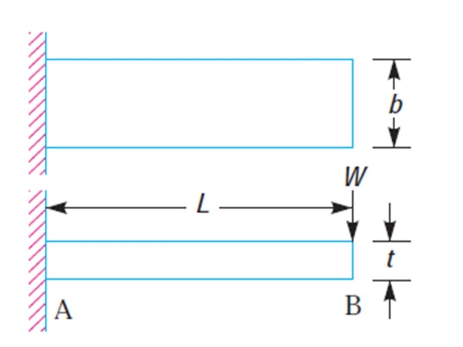
Figure 1.1: Flat spring cantilever type

The bending stress and deflection of this flat plate is calculated using following equation.

Bending stress in  spring:

Deflection of spring:–

6WL

σ =  Bt2

4WL3

δ =  EBt3

(1.1)

(1.2)

In the bending moment, top fiber will be in tension and bottom fibers in compres- sion, but the shear stress is zero at the extreme fibers and maximum at the center. Bending stress zero at the centre where shear stress maximum at the center as shown in fig 1.2.

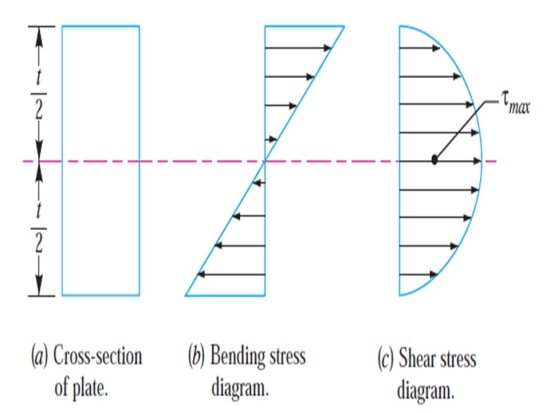
Figure 1.2: (a) Cross-section of plate (b) Bending stress (c)Shear stress diagram

If we consider the spring as simply supported beam the length is 2L and load 2W as shown in fig 1.3.The bending stress and deflection of this flat plate is calculated using following equation.

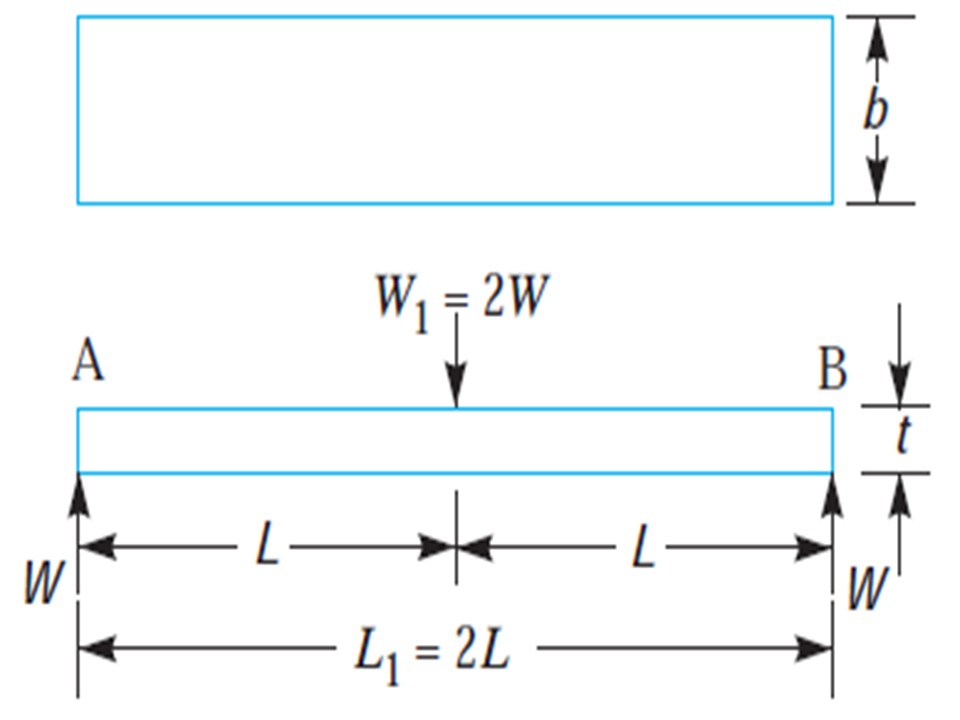
Figure 1.3: Flat spring simply supported beam type

The bending stress and deflection of this flat plate is calculated using following equation.

Bending stress in  spring:

6WL

σ =  Bt2

(1.3)

Deflection of spring:

WL3

δ =

3EI

(1.4)

If we consider n-strips cantilever beam having width b and thickness t then we can use equation 1.5 and 1.6. and n-strips cantilever beam is shown in fig 1.4.The bending stress and deflection of this flat plate is calculated using following equation.

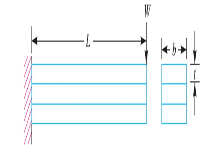
Figure 1.4: Flat spring simply supported beam type

Bending stress in  spring:

6WL

σ = nBt2

(1.5)

Deflection of spring:

4WL3

δ  = nEBt3

(1.6)

The above relations give the stress and deflection of a spring of  uniform cross section. The stress at such a spring is maximum at the support. If we  consider triangular plate is used as shown in fig.1.5 the stress will be uniform throughout. If this triangle plate is cut into strips of width and Fitted one below the other as shown fig 1.5 to form a graduated or laminated leaf spring, then The bending stress and deflection of this flat plate is calculated using following equation.

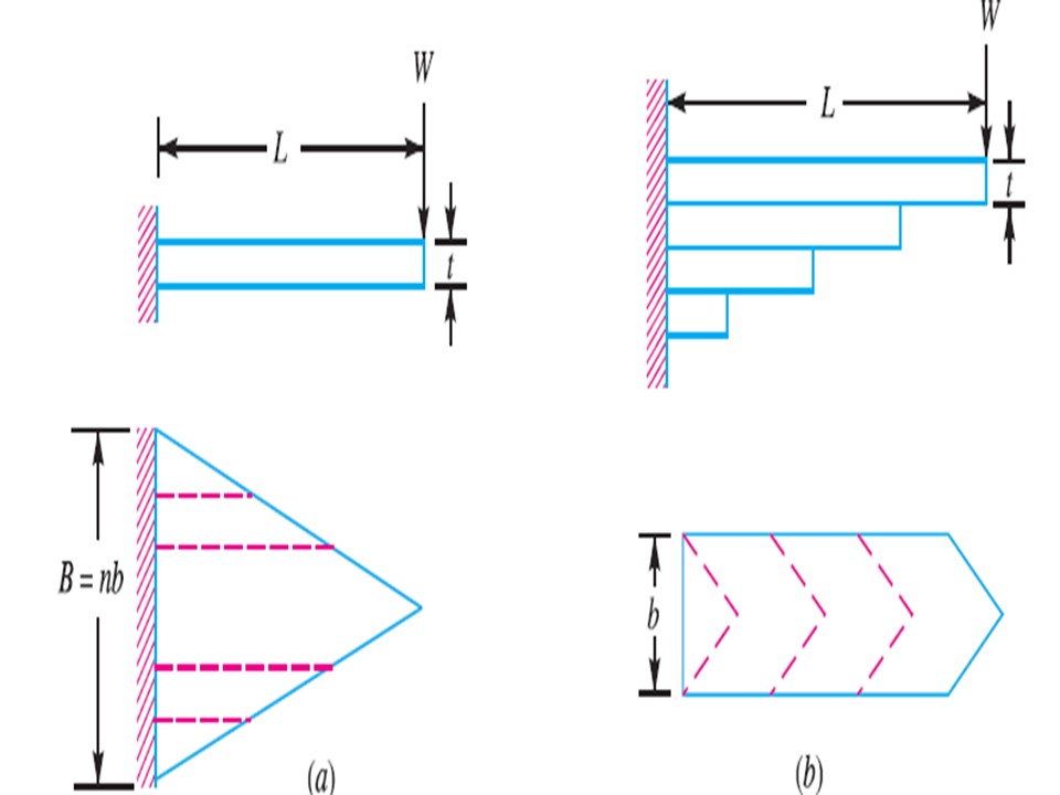
Figure 1.5: Laminated leaf spring

Bending stress of leaf spring;

6WL

σ = nBt2

(1.7)

Deflection of spring:

6WL3

δ  = nEBt3

(1.8)

Construction of Leaf Spring

A Leaf spring is generally used in automobiles is of semi elliptical form shown in fig.1.6. It is built up of a number of plates. The leaves are usually given an initial curvature or cambered so that they will  tend to straighten under the load .The leaves are held together by means of a band shrunk around them at the center or by a bolt passing through the center. Since the band  exerts a stiffening and strengthening effect, therefore  the effective length of the spring for  bending will be the overall length of the spring  minus width of band.  In case of a  center bolt, two-third distance between center of bolt should be subtracted  from the overall length of the spring in order to find effective length. The spring is clamped to the axle housing by means of U-bolts. The longer leaf known as main leaf or master leaf has its ends formed in the formed in the shape of an eye through which the bolts are passed to secure the spring to its supports. Usually the eyes, through which the spring is attached to the hanger or shackle, are provided with the bushing of some  antifriction materials such as bronze or rubber. The other leaves of the spring are known graduated leaves. In order to prevent digging in the adjacent leaves, the ends of graduated leaves are trimmed in various forms as shown in fig.1.6. Since the master leaf has to with stand vertical bending loads as well as loads due to sideways of the vehicle and twisting, therefore due to presence of stresses caused by these loads, it is usual to provide two full length leaves and the rest graduated as shown in fig.1.6.

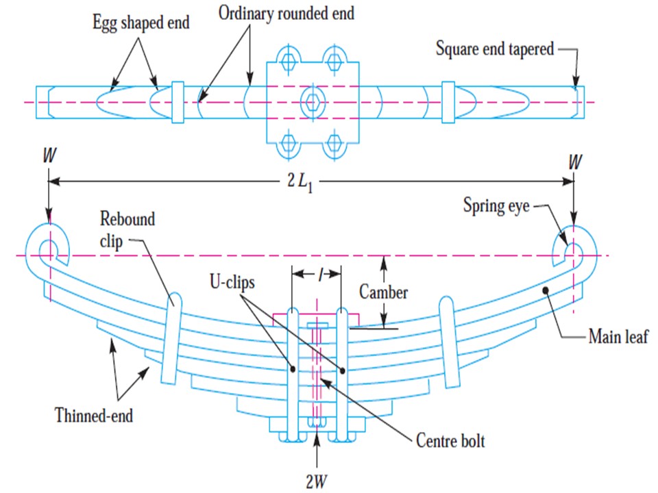
Figure 1.6: Semi elliptical leaf spring

Table 1.1: Dimension for center bolt

Width of leaves mm	Dia. Of center bolt (mm)	Dia. Of head bolt (mm)	Length of bolt head (mm)
Up to and including 65	8 or 10	12 to 15	10 or 11
Above 65	12 or16	17 or 20	11

Table 1.2: Dimension for clip, rivet , bolt

Spring width mm	Clip section (b * t) mm*mm	Dia. Of rivet (d1) mm	Dia. Of bolt(d2) mm
Under 50	20*4	6	6
50, 55 and 60	25*5	8	8
65,70,75 and 80	25*6	10	8
90,100 and 125	32*6	10	10

1.6 Standard Sizes of Suspension Leaf Spring

Standard nominal widths are: 32,40,45,55,60,65,70,75,80,90,100 and 125 mm.

Standard nominal thickness are:  3.2,4.5,5,6,6.5,7,7.5,8,9,10,11,12,14 and 16 mm.

At the eye, the following bore diameter are recommended- 19,20,22,23,25,27,28, 30,32,35,38,50,55 mm.

Dimension for the centre bolts, if employed, shall be as given in the table 1.1.

Minimum clip sections and the corresponding sizes of rivets and bolts used with the clips shall be as given in the table 1.2.

Design of Multi LeafSpring

Properties for Steel and Composite Material

Consider loaded mini truck leaf spring load carrying 80000 N, length 1025 mm , Width 60 mm, thickness 16 mm, Camber distance 90.8 mm. and number of the leaves are 10.The material properties for steel and composite materials are as shown in table 3.1 and 3.2

Table 3.1: Material properties of Steel materials

parameter	values
Material Selected	Steel(Sup9)
Young’s Modulus, E	2.1*10ˆ5 N/mm2
Possion’s Ratio	.266
BHN	400-425
Tensile  strength Ultimate	1272 Mpa
Tensile strength Yield	1158 Mpa
Density	7850 Kg/m3

20

Table 3.2: Properties for composite material

parameter	values
Exx	206.85 Mpa
Eyy	517.12 Mpa
Ezz	517.13 Mpa
Mx	.26
My	.26
Mz	.26
Gxy	258.6 Mpa
Gyz	258.6 Mpa
Gxz	258.6 Mpa
Density	1602 kg/m3

Design Calculation

In design of leaf spring these condition must be satisfy,

σa“σ δmax“δ

Bending  Stress Calculation

If σa“σthen Design is safe.

Allowable Stress:

σmax

σa = FactorofSafety = 508.8MPa (3.1)

Bending Stress:

6WL

σ =  nbt2

= 187.7 MPa (3.2)

Here σa“σso design is safe.

Deflection Calculation

If δmax“δthen Design is safe.

Max. Deflection:

σL2

δmax = 6tE  = 16.35mm (3.3)

Deflection of spring

6PL3

δ =

(3nf + 2ng )Ebt3

= 6.69mm (3.4)

Here δmax“δso design is safe.

Spring Rate Calculation

p

K= = 1347.3053N/mm (3.5)

δ

Radius of Curvature

L2

R =

8δ0

= 1446.34mm (3.6)

Static Analysis in LeafSpring

A stress-deflection analysis is performed using finite element analysis (FEA). The complete Steps of analysis has been done using ANSYS. To conduct finite element analysis, the general process of FEA is divided into three main phases.

• Preprocessor
• Solution
• Postprocessor

Preprocessor

The preprocessor is a program that processes the input data to produce the output that is used as input to the subsequent phase (solution). Following are the input data that need to be given to the preprocessor

• Type of analysis
• Geometric modal
• Type of Element
• Material properties
• Meshing
• Loading Conditions
• Boundary Conditions

Solution

Solution phase is completely automatic. The FEA software generates the element matrices, computes nodal values and derivatives, and stores the result data in files. These files are further used by the subsequent phase (postprocessor) to review and analyze the results through the graphic display and tabular listings.

Postprocessor

The output from the solution phase is in the numerical form and consists of nodal values of the field variable and its derivatives. material used for the leaf spring for analysis is structural steel, which has approximately similar isotropic behavior and properties as compared to SUP9.

Meshing

Meshing is the process in which your geometry is spatially discredited into elements and nodes. This mesh along with material properties is used to mathematically represent the stiffness and mass distribution of the structure. The mesh has been generated automatically. The default element size is determined based on a number

of factors including the overall model size, the proximity of other topologies, body curvature, and the complexity of the feature. If necessary, the fineness of the mesh is adjusted up to four times (eight times for an assembly) to achieve mesh. As shown in fig 4.1 Number of elements used are 56568 and and number of nodes used are 286796.

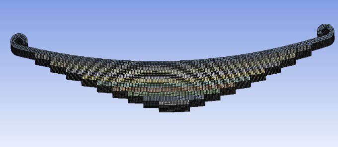
Figure 4.1: Meshing

Sizing Control

The sizing control sets the element size  for a selected body, face, edge. The number of divisions along an edge. The element size within a  user of influence that can include a selected body, face, edge, or vertex. This control is recommended for local mesh sizing. The control must also be attached to a coordinate system if it is to be scoped to anything other than a vertex.

Boundary Conditions

The boundary condition is the collection of different forces, pressure, velocity, sup- ports. Applying boundary condition is one of the most typical processes of analy- sis. A special care is required while assigning loads and constraints to the elements. Boundary condition of the spring involves the fixation of  one of the revolute joint and applying displacement support at the other end of leaf spring. Loading conditions involves applying a load upper side at the centre of the main leaf.

Result

Static analysis result in leaf spring using steel material

1. Make simplified 3D model leaf spring in SolidWorks.
2. Make and save above modal STEP format and importing in to ANSYS.
3. After importing modal provide material properties as table 3.1.
4. After providing material properties Make  mesh.
5. After providing mesh input boundary  condition one end fixed and other end X and Y axis displacement is given.Loading conditions involves applying a load upper side at the centre of the bottom leaf.
6. After Solving the model for static structural analysis and bending stress and deflection as shown in fig 4.2 to 4.3.

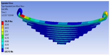
Figure 4.2: Von-Mises stress in steel material leaf spring

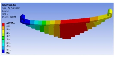
Figure 4.3: Deflection in steel material leaf spring

Static analysis result in leaf spring using composite materials

For composite material same Steps has been adopted as steel material except material properties. After solving the model for static structural analysis Von-Mises stress plot is as shown in fig. 4.4. The deflection plot for the same model is as shown in fig. 4.5.

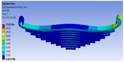
Figure 4.4: Von-Mises stress in composite material leaf spring

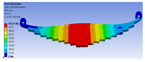
Figure 4.5: Deflection in composite material leaf spring

If we consider mono leaf spring and taken same dimension as multi leaf spring only thickness is varies by considering same deflection and same von-Mises stress. Mono composite leaf spring weight reduction is Gained 90.09%. Using HyperMesh, considering mono leaf spring as shown in fig.4.6 maximum Von-Misses stress Gained 190 MPa and maximum deflection is Gained as shown in fig. 4.7 is 7.11 mm. The thickness for mono leaf spring is derived 36 mm.

Figure 4.6: Von-Mises stress in composite material Mono leaf spring using HyperMesh

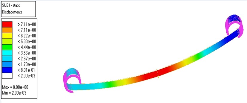
Figure 4.7: Displacement in composite material Mono leaf spring using HyperMesh

Results table

As shown in table 4.1 deflection value analytically 6.60 mm and FEA 6.34 mm so 5.56% difference and bending stress value analytically 187.68 MPa and 206.1 MPa so 9.064% difference.

Table 4.1: Static result analytical and FEA comparison

Parameter	Analytical	FEA	Difference
Deflection	6.69 mm	6.34 mm	5.56%
Bending Stress	187.7 Mpa	206.1 Mpa	9.06%

As shown in table 4.2 compression of  mass properties steel and composite material. Composite material mass reduction is 90.094% Gained.

Table 4.2: Static steel and composite result comparison

Parameter	Steel	Composite	Difference
Bending Stress	187.5 Mpa	135 Mpa	5.8%
Mass	44.494 kg	5.1 kg	90.09%

Fatigue Analysis and Modal Analysis in Leaf Spring

Fatigue Analysis

Introduction

Fatigue occurs when a material is subjected to repeated loading and unloading. If the loads are  above a certain threshold, microscopic cracks will begin to form at the stress concentration such as the surface and grain interfaces. Eventually a crack will reach a critical size, and the structure will suddenly fracture. The shape of the structure will significantly affect the fatigue life; square holes or sharp corners will lead to elevated local stresses where fatigue cracks can initiate. Round holes and smooth transitions or fillets are therefore important to increase the fatigue strength of the structure. 30

Characteristics of fatigue

• In metals and alloys, when there are no macroscopic or microscopic discon- tinuities, the process starts with dislocation movements, eventually forming persistent slip bands that nucleate short cracks.
• Macroscopic and microscopic discontinuities as well as component design fea- tures which cause stress concentration (keyways, sharp changes of direction etc.) are the preferred location for starting the fatigue process.
• Fatigue is a stochastic  process, often showing considerable scatter even in con- trolled environments.
• The greater the applied stress range, the shorter the life.
• Fatigue life scatter tends to increase for longer fatigue lives.
• Damage  is cumulative. Materials do not recover when rested.
• Fatigue life is influenced by a variety of factors, such as temperature, surface finish, microstructure, presence of oxidizing or inert chemicals, residual stresses, contact (fretting), etc.

Fatigue Analysis

Analysis of fatigue can be carried out by in three basic Method:

1. Strain Approach
2. Stress Approach
3. Crack  Propagation

Strain life Approach three is again classified into three methods as:

1. Morrow Approach
2. Mean Approach
3. SWT  (Smith-Watson-Topper)Approach

Strain controlled tests are always conducted in axial loading. Deflections are con- trolled and converted into strain. The resulting forces are measured to compute the applied stress. Metals undergo transient behavior when they are first cycled. In this

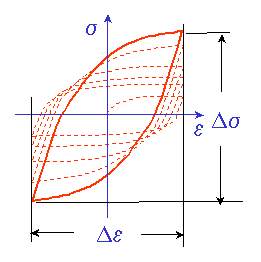
Figure 5.1: strain approach cycle

Before plotting the strain vs. fatigue life, the total strain that was controlled during the test is divided into the elastic and plastic part. The elastic strain is computed as the stress range divided by the elastic modulus. Plastic strain is obtained by sub- tracting the elastic strain from the total strain. The total strain is then obtained by adding the elastic and plastic  portions of the strain to obtain a relationship between the applied strain and the fatigue life.

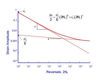
Figure 5.2: strain – reversals graph

The material deformation during a fatigue test  is measured in the form of a hysteresis loop.  After the initial transient behavior the material stabilizes and the same hysteresis loop is obtained for every loading cycle. Each strain range tested will have a corresponding stress range that is measured. The cyclic  stress strain curve is a plot of all of this data.

Fatigue Material Properties :

The fatigue material properties are described in table 5.1.

Table 5.1: Fatigue Material properties

Parameter	Values
Material Selected	Steel(Sup9)
Young’s Modulus, E	2.1*10ˆ5 N/mm2
Tensile  strength Ultimate	1272 Mpa
Tensile strength Yield	1158 Mpa
Fatigue Strength co-efficient	2063 Mpa
Fatigue  Strength exponent	-.08
Fatigue  ductility coefficient	9.56
Fatigue ductility exponent	-1.05

The Equation for strain life approaches are as follows.

Morrow Approach:

sa =

σf (2N∗)b

E

+ sf(2N σm

∗)c

(5.3)

Nf = N∗(1 −

) (5.4)

σf

Mean Approach:

sa =

σf − σm (2N )b

E f

+ sf(2Nf)c

(5.5)

SWT  (Smith-Watson-Topper)  Approach:

saσmax =

σf 2

(2Nf)2b

E

+ sfσf(2Nf)

b+c

(5.6)

Loading Information

Loading is major input for the finite element based fatigue analysis. Unlike static stress, which is analyzed with calculations for a single stress state, fatigue damage occurs when stress at a point  changes over time.

Here non-constant  amplitude, proportional loading has been considered within the ANSYS. Fatigue Module uses a“quick counting” technique to substantially reduce runtime and memory. In quick counting, alternating and mean stresses are sorted into bins before partial damage is calculated.

Fatigue Analysis using FEA

The Steps for fatigue analysis using FEA is explained as follows.

• Make simplified 3D model leaf spring in  SolidWorks.
• Make and save above modal STEP format and importing in to HyperMesh.
• After importing modal and provide material properties as table 3.1.
• After providing material properties Make mesh.
• After providing mesh input boundary condition one end fixed and other end X and Y axis displacement is given. Loading conditions involves applying a load upper side at the centre of the bottom leaf.
• After Solving the model for fatigue analysis and obtain life cycle as shown in fig 5.3 to 5.5.

As shown in fig 5.3, 5.4 and 5.5 are FEA result of strain based approach. Using three strain approach and calculated life cycle for leaf spring. Fig 5.4 is for Morrow approach, Fig. 5.5 is for Mean approach and Fig 5.6 for SWT approach to calculate fatigue life.

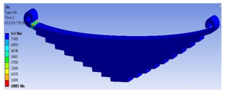
Figure 5.3: Fatigue life calculated using Morrow Approach for Leaf Spring

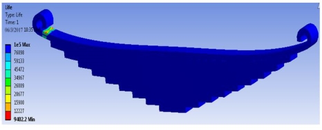
Figure 5.4: Fatigue life calculated using Mean Approach for Leaf Spring

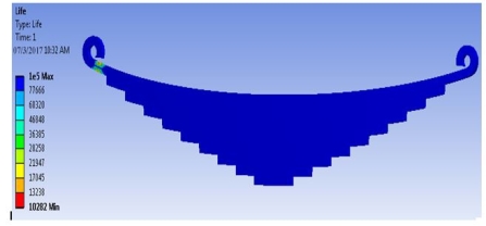
Figure 5.5: Fatigue life calculated using SWT Approach for Leaf Spring

Fatigue Analysis Result

Using strain based approach fatigue life has been calculated using analytically as well as FEA. The %difference is given in table 5.2.

Table 5.2: Predicted fatigue life using strain life approach

Approach	Analytical(life  cycle)	FEA (life cycle)	%Difference
Mean	8.9e4	9.40e4	5.31
Morrow	1.2e4	1.0081e4	16
SWT	1.15e4	1.02e4	11.13

Modal Analysis

Modal analysis is the field of measuring and analyzing the dynamic response of struc- tures and or fluids when excited by an input. The goal of modal analysis in structural mechanics is to determine the natural mode shapes and frequencies of an object or structure during free vibration. It is common to use the finite element method (FEM) to perform this analysis because, like other calculations using the FEM, the object being analyzed can have arbitrary shape and the results of the calculations are acceptable. The types of equations which arise from

modal analysis are those seen in eigen systems. The physical interpretation of the eigenvalues and eigenvectors  which come from solving the system are that they rep- resent the frequencies and corresponding  mode shapes. Sometimes, the only desired modes are the lowest  frequencies because they can be the most prominent modes at which the object will vibrate, dominating all the higher frequency modes..

FEA Eigen System

For the most basic problem involving a linear system  elastic material the obeys hook’s law the matrix equation takes the form of a dynamic three a dimensional spring mass system. The generalized equation of motion is given as:

[M]*[U¨ ] + [C]*[U˙ ] + [K]*[U] = [F]

where,

[M] is mass matrix

[U¨ ] Second  derivative Accerlation [U]  Displacement

[U˙ ] velocity

[C] Damping matrix [K] Stiffens matrix [F] Force vector.

The general with nonzero damping is a quadratic  eigenvalue problem. Howerver, for vibrational model analysis the damping is generally  ignored leaving only the 1stand 3rdterms on the hand side:

[M][U¨ ] + [K][U] = 0

This is the general from of the eigen system encountered in structure engineering

using the FEM vibration sollutoin of the structure  harmonic motion is assumed so that [U¨ ] is taken to equal λ[U],where λis an eigenvalue and the equation reduce to:

[M][U¨ ]λ+ [K][U] = 0

In construct , the equation for static problem is: [k] [U] = [F]

Which is expected when are terms having a time derivatives are set to zero.

FEA Steps for Modal Analysis

The Steps for model analysis using FEA is described as follows.

• Make simplified 3D model leaf spring in SolidWorks.
• Make and save above modal STEP format and importing in to HyperMesh.
• After importing modal provide material properties as table 3.1.
• After providing material properties Make  mesh.
• After providing mesh input boundary condition one end fixed and other end X and Y axis displacement.
• After Solving the model for modal analysis and obtain mode shape as shown in fig 5.7 to 5.10.

Different mode shape having different natural frequencies as shown in fig. 5.6 to 5.10. Here first five shapes has been found.

Figure 5.6: First mode shape natural frequency using hyperMesh

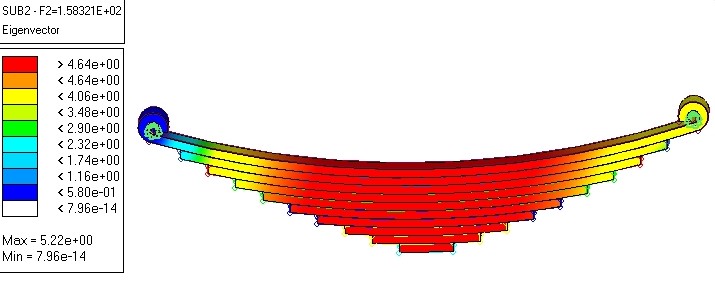
Figure 5.7: Second mode shape natural frequency using hyperMesh

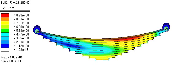
Figure 5.8: Third mode shape natural frequency using hyperMesh

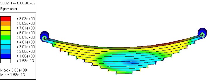
Figure 5.9: Fourth mode shape natural frequency using HyperMesh

Figure 5.10: Fifth mode shape natural frequency using HyperMesh

Size Optimization

Size optimization  is part  of the field of optimal control theory. The typical problem is to find the shape which is optimal in that it minimizes a certain cost functional while satisfying given constraints. In many cases, the functional being solved depends on the solution of a given partial differential equation defined on the variable domain. Shape optimization problems are usually solved numerically, by using iterative meth- ods. That is, one starts with an initial guess for a shape, and then gradually evolves it, until it morphs into the optimal shape.

In mathematics and computer science, an optimization problem is the problem of finding the best solution from all feasible solutions. Optimization problems can be divided into two categories  depending on whether the variables are continuous or dis- crete. An optimization problem with discrete variables is known as a combinatorial optimization problem. In a combinatorial optimization problem, we are looking for an object such as an integer, permutation or graph of a finite (or possibly countable infinite) set.

Continues optimization problem

The standard form of optimization problem is minimization f(x) subjected to

42

gi(x)≤0 i= 1……m

hi(x)≥0 i= 1……n

where f(x): Rn −→R is the objective function to be minimized over the variable , gi(x)≤0 are called inequality constraints, and

hi(x)≥0 are called equality  constraints.

By convention, the standard form defines a minimization problem. A maximization problem can be treated by negating the objective function.

Steps for Size Optimization

The Steps for optimization is described as follows.

• Make simplified 3D model leaf spring in SolidWorks.
• Make and save above model STEP format and importing in to HyperMesh.
• After importing model provide material properties as table 3.2.
• After providing material properties Make  mesh.
• After providing mesh input boundary condition one end fixed and other end X and Y axis displacement is given. Loading conditions involves applying a load upper side at the centre of the bottom leaf.
• After boundary condition Make in analysis page optimization.
• In optimization constraints considered is stress and objective function mini- mization mass.
• After solving the model for size optimization and obtain reduction thickness as shown in fig 6.3.

Before optimization

See the Fig. 6.1 and 6.2 are the result of before optimization. The weight of the spring is 5.18 kg and thickness is 36 mm.

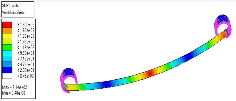
Figure 6.1: von misses stress in mono leaf spring using hyper mesh

Figure 6.2: Deflection in mono leaf spring using hyper mesh

After optimization

As shown in Fig. 6.3 is the result of After optimization. After five iteration weight in leaf spring reduced up to 5.01 kg and thickness 35 mm obtained. So 1 mm thickness reduction is Gained.

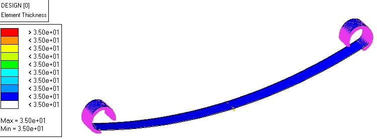
Figure 6.3: After Optimization mono leaf spring using hyper mesh

Residual Stress Calculation

Residual stress is defined as “the stress resident inside a component or structure after all applied forces have been removed”. Compressive  residual stress acts by pushing the material together, while tensile residual stress pulls the material apart.

Mathematically, compressive stress  is negative and tensile stress  is positive. Stresses can also be characterized as normal stresses that act perpendicular to the face of a material and shear stresses that act parallel to the face of a material. There is a total of 6 independent stresses at any point inside a material represented by σijwhere i is the direction that the stress is acting and j is the face the stress is acting on.

Residual stresses or locked-in stresses can be defined as those stresses existing within a body in the absence of external loading or thermal  gradients. In other words residual stresses in a structural material or component are those stresses which exist in the object without the application of any service or other external loads.

Residual stress is usually defined as the stress which remains in mechanical parts which are not subjected to any outside stresses. Residual  stress exists in practically all rigid parts, whether metallic or not (wood, polymer, glass,ceramic, etc). It is the result of the metallurgical and mechanical history of each point in the part and the part as a whole during its  manufacture. It exists at different levels, generally divided into three, depending on the scale on which the stress is observed.

46

Factors that cause residual stresses

Residual stresses can be present in any  mechanical structure because of many causes. Residual stresses may be due to the technological process used to make the compo- nent. Manufacturing processes are the most common causes of residual stress. Virtu- ally all manufacturing and fabricating processes such as casting, welding, machining, molding, heat treatment, plastic deformation during bending, rolling or forging intro- duce residual stresses into the manufactured object. Residual stress could be caused by localized yielding of the material, because of a sharp notch or from certain surface  treatments like shot peening or  surface hardening. Among the factors that are known to cause residual stresses are the development of deformation gradients in various sections of the piece by the development of thermal gradients, volumetric changes arising during solidification or from solid state transformations, and from  differences

in the coefficient of thermal expansion in pieces made from different materials. Thermal residual  stresses are primarily  due to differential  expansion when a metal is heated or cooled. The two factors that  control  this are thermal treatment (heating or cooling) and restraint. Both the thermal treatment and restraint of the component must be present to generate residual stresses.

When any object is formed through cold working, there is the possibility for the de- velopment of residual stresses.

A good  common example of mechanically applied residual stresses is a bicycle wheel. A bicycle wheel is a very light and strong because of the way in which the com- ponents are stressed. The wire spokes are radial aligned and tightening the spokes Makes tensile radial stresses. The spokes pull the rim inward, creating circumfer- ential compression stresses in the rim. Conversely, the spokes pull the tubular hub outward. If the thin spokes were not under a proper tensile preloaded the thin wire spokes could not  adequately support the load of the rider.

Residual stress Calculation in leaf spring

Residual stress calculation  in different leaves of leaf spring has been described below. As shown in fig 7.1 one leaves of  leaf spring and below calculation is done for single leaves spring.

For single leaf of spring, residual stress   calculation method  has been explained. Fig.7.1 is shows  single leaf of spring.

CG of the leaves y = 28.80 mm

I = Moment of inertia about y-Axis

db3

I =

12

= 2.04e6mm4 (7.1)

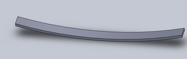
Figure 7.1: Single Leaf of the Spring

WL2

M =

8

= 2.162e6N∗mm (7.2)

σ = M ∗ Y

I

= 305.22MPa (7.3)

Max.ResidualStress= YieldStress−305.22 = 852.77Mpa (7.4)

Table 7.1 shows bending stress and residual stress for all 10 leaves of leaf spring.

Table 7.1: Residual stress calculation

Leaves no.	y   mm	L   mm	M   N.mm	Bending stress   (σ  (MPa))	Residual stress (σmax(MPa))	Residual stress (σmin(MPa))
1	46.78	1025	2.402e6	390.158	767.842	-767.842
2	28.80	922.5	2.042e6	305.22	852.77	-852.77
3	25.36	820	1.91e6	238.68	919.32	-919.32
4	20.25	717.5	1.68e6	166.76	991.24	-991.24
5	16.89	615	1.44e6	119.339	1038.661	-1038.66
6	14.17	512.5	1.20e6	83.43	1074.57	-1074.57
7	12.89	410	9.6e5	60.718	1097.282	-1097.28
8	11.10	307.5	7.2e5	39.214	1118.786	-1118.78
9	10.15	205	4.8e5	23.789	1134.211	-1134.21
10	9.05	102.5	2.4e5	10.647	1047.353	-1047.35

Conclusion and future  Scope

Conclusion

The design and static structural analysis of steel leaf spring and laminated composite leaf spring has been carried out. Comparison has been made between laminated composite leaf spring with steel leaf spring having same design and same load carrying capacity. From that 79.9 % mass reduction in composite material has been Gained for the same number of leaves. The fatigue  life has been calculated using analytically as well as using ANSYS for steel leaf spring. The size optimization has been carried out for further mass reduction of composite leaf spring. From that 90 % mass reduction has been Gained using mono composite leaf spring compared to steel multi leaf spring.