The Effect of External Debt in Economic Growth Case Study of Mauritania
Info: 15675 words (63 pages) Dissertation
Published: 13th Dec 2019
THE EFECT OF EXTERNAL DEBT IN ECONOMIC GROWTH
CASE STUDY of Mauritania: (VECM Analysis)
Abstract
The study attempts to investigate the impact of external debt flows on economic growth in Mauritania over a period of 34 years starting from 1980 to 2014 by using Vector Error Correction Model (VECM). The findings reveal that there is positive impact of external debt on economic growth in the long-run. However, the results indicate a negative relation between services of debt and economic growth both in short and long term. This could be explained by the fact that foreign capital flow is used to enhance the government ability to create a competitive business environment by expanding the national spending. On the other hand, the services of debt constitute a burden on national economy. The country has to spend a significance proportion of its GDP to pay off these services. Therefore, Mauritanian government should seek to improve its national resource and capability to finance its economy transformation and cut down the amount of external debt and ultimately reduce debt services.
Key words: Gross domestic product, External debt, Service debt, investment .VECM, Mauritania.
Contents
ACKNOWLEDGEMENTS………………………………….
Abstract……………………………………………..
1 INTRODUCTION………………………………………
1.1 Introduction………………………………………
1.2 Review of Conceptual and Definitions Issues……………………
1.2.1 Origin of Debt Crisis in LDC s:………………………..
1.2.2 Why Countries Borrow…………………………….
1.2.3 Origin of Mauritanian’s External Debt……………………
1.2.4 Mauritania External Debt Relief……………………….
1.3 HIPC debt in Sub-Saharan Africa………………………….
2 Literature Review………………………………………
2.1 Review of Conceptual and Definition Issues……………………
2.2 Review of Theoretical Issues…………………………….
2.2.1 The Dual-gap theory………………………………
2.2.2 External debt and Economic growth……………………..
2.2.3 The Dependency Theory……………………………
2.3 Theoretical of literature………………………………..
2.4 Empirical of Literature………………………………..
3 The methodology of this research…………………………….
3.1 specification of the model………………………………
3. 2 Techniques of Estimation………………………………
3.2.1 Unit Root Test………………………………….
3.2.2 Co-integration test……………………………….
3.2.3 Vector Error Correction Model………………………..
3.2.4 G ranger Causality test…………………………….
3.2.5 Impulse Response Analysis………………………….
3.3 The hypotheses to be tested in the course of this study include………….
4 Data analysis & interpretation………………………………
4.1 introduction……………………………………….
4.2 Data Source and Description of variables……………………..
4.3 Descriptive analysis………………………………….
4.4 Vector Error Correction Estimates test……………………….
4.4.1 log selection:…………………………………..
4.4.2-Test of co-integration……………………………..
4.4.3 G ranger Causality test…………………………….
4.5.4 VECTOR ERROR CORRECTION MODEL (VECM) Test result……
4.5 Impulse Response result analysis…………………………..
5 Conclusion and recommendation…………………………….
Reference…………………………………………….
Appendix…………………………………………….
Appendix A: vector error correction model test result…………………
Appendix B: Wald Test………………………………….
Appendix C: Co integration test result………………………….
1 INTRODUCTION
1.1 Introduction
1950’s and 1960’s are most often described as the “golden years” for developing countries in economic development literature because of the rate of economic growth which was not just high but also internally generated. In the above years these LDC increased their investment reliance on external resources however most of the growth in the 1970s was “debt led” and this led to persistent current account deficits with massive borrowings from the international money and capital market (ICM) to bridge payment gaps. External debt has increased steadily over the years in developing countries and as such an analysis of the role external debt plays in economic growth and development is paramount. Aside from being an ardent booster of growth external debt has also been known to cause a number of problems for developing countries. The increases in external debt over the years in developing countries has brought the issue of external debt out of hiding and has become a matter of concern both to the international and local community. The need to constantly borrow as a means of financing has brought about an increasing literature among various economists.
Mauritania, like most other less developed countries (LDC) has been classified by the World Bank among the severely indebted low income countries since 1992. The nation’s inability to meet all of its debt service payment constitutes one of the serious obstacles to the inflow of external resources into the economy. The accumulation of debt service arrears worsened by high interest payments has catapulted the external debt stock to extremely high levels and all efforts to substantially reduce the debt has been unsuccessful. This chapter therefore carries out an extensive literature review on the subject matter of external debt and economic growth by looking at conceptual and definitions issues, theoretical issues, empirical and methodological issues and summary.
1.2 Review of Conceptual and Definitions Issues
The act of borrowing creates debts and this debt may be domestic or external. The focus of this study is on external debt which refers to that part of a nation’s debt that is owed to creditors outside the nation. Ar none ET AL (2005) defines external debt as that portion of a country’s debt that is acquired from foreign sources such as foreign corporations, government or financial institutions. According to (Ogbeifin, 2007), external debt arises as a result of the gap between domestic savings and investment. As the gap widens, debt accumulates and this makes the country to continually borrow increasing amounts in order to stay afloat. He further defined Mauritania’s external debt as the debt owed by the public and private sectors of the Mauritanian economy to non-residents and citizens that is payable in foreign currency, goods and services.
Debt crisis occurs when a country has accumulated a huge amount of debt such that it can no longer effectively manage the debt which leads to several mishaps in the domestic political economy (Adejuwon ET AL). Mimiko (1997) defined debt crisis as a situation whereby a nation is severely indebted to external sources and is unable to repay the principal of the debt…
1.2.1 Origin of Debt Crisis in LDC s:
Prior to 1979 most countries, particularly the five major LDC s (Brazil, Mexico, Venezuela, Spain, Argentina), which together owed about half of total external debt in 1979 encountered no serious problems in meeting debt service requirement. However, by 1980 a number of LDC s, including Peru, Bolivia, Sudan, Turkey, Zaire, and Zambia, had experienced serious difficulties in coping with their debts. More ominously, there were indications even by the early 1980s that at least one of the large borrowers (Brazil) had reached or surpassed its capacity to service further debt, as a combination of doubling of import prices for oil, Obligations from past external borrowings
And rising protection in industrial countries left little foreign exchange to pay for imports.
By 1982 and 198 concern over an impending crisis in LDC debts was pervasive, both in capital-exporting and capital-importing nations. The total value of outstanding LDC debts to commercial banks had nearly tripled from $160 billion in 1979 to almost $460 billion in 1983.More and more countries each month experienced difficulties in servicing their debt .many oil-importing LDC s had initially in 1974 and 1975 and again in 1979 and 1981 to allow them to cope with the rise in oil prices from $3 per barrel to nearly $36 over that period. But with the onset of the deep world recession of the early eighties, and the rise of renewed protectionist policies in industrial countries, debt service capacity in those nations fell sharply with their exports. For all LDC s, the ratio of debt to exports had reached 131 percent and debt service (interest payments and repayments of principal) as a percent of exports was 19 percent. Oil exporters had only just begun to feel the pinch in 1982. Many, such as Indonesia and Nigeria, had World oil market softened gradually from 1982 through 1984, and then rapidly in 1985 and 1986, many such nations were beginning to face debt service difficulties as well.
A crisis atmosphere prevailed in 1982 and 1983; large debtor nation such as Argentina and Brazil appeared to be on the on the verge of default. The press was full of talk of an imminent collapse of several large American and European banks, not to mention the entire international monetary system. The so-called”crisis appeared to abate in 1982 and 1985, with the recovery of the world economy and far-reaching structural changes in international financial markets. These served fundamentally to alter the future lending behavior of commercial banks and to blur the distinctions between banks and other financial institutions. The first change was the greater readiness of the banks to accede to postponement of scheduled debt repayments from debtor LDC s. Indeed, there was little alternative but to so, since the only other option open to many LDC s was outright default on their loan obligation, as in fact many did during the Great Depression of the 1930s.By 1986,more than forty LDC, Including virtually every Latin American country, had been forced to postpone scheduled debt payments. No country had yet defaulted outright, in spite of the onerous debt service burdens facing many, rather, the debts were rescheduled through negotiations, sometimes of a delicate nature. Still the burden remains of servicing an LDC debt (both commercial debt and official debt) that is estimated at $1.01 trillion in 1986.half of which is owed to private lenders. And by mid-1986, the debt service capacities of several formerly “safe” LDC oil exporters, including Indonesia and Nigeria, had weakened substantially, as noted earlier.
LDC. By 1986, 1 powerful “scissors” effect of escalating debt service ratios and declining capital inflows from new loans had developed. The outflow of foreign exchange required to service debt diverted savings that otherwise would have been available for domestic investment and imports needed to support the recoveries of LDC economics. The outflow had become substantial by 1985: LDC debtor countries paid the equivalent of %50 billion in interest alone too overseas creditors in 1985; this was $22 billion more than the new loans they received in that year. The scissors effect was particularly damaging in Africa.Net external borrowing by Sub-Saharan African countries fell from $14 billion in 1982 to only $2 billion in 1985.While most media attention has focused on the debt problem of Latin American countries, money experts believe that the impact of debt crisis on people has been much more severe in Africa.
1.2.2 Why Countries Borrow
Generally the need for public borrowing arises from the recognized role of capital in the developmental process of any nation as capital accumulation improves productivity which in turn enhances economic growth. There is abundant proof in the existing body of literature to indicate that foreign borrowing aids the growth and development of a nation. Soludo (2003) was of the opinion that countries borrow for major reasons. The first is of macroeconomic intent that is to bring about increased investment and human capital development while the other is to reduce budget constraint by financing fiscal and balance of payment deficits. Furthermore (Ibadan and Uga, 2007) stressed the fact that countries especially the less developed countries borrow to raise capital formation and investment which has been previously hampered by low level of domestic savings. Ultimately the reasons why countries borrow boils down to two major reasons which are to bridge the “savings-investment” gap and the “foreign exchange gap”. Chenery (1966) pointed out that the main reason why countries borrow is to supplement the lack of savings and investment in that country. The dual-gap analysis justifies the need for external borrowing as an attempt in trying to bridge the savings-investment gap in a nation. For development to take place it requires a level of investment which is a function of domestic savings and the level of domestic savings is not sufficient enough to ensure that development take place (Oloyede, 2002). The second reason for borrowing from overseas is also to fill the foreign exchange (imports-exports) gap. For many developing countries like Mauritania the constant balance of payment deficit have not allowed for capital inflow which will bring about growth and development. Since the foreign exchange earnings required to finance this investment is insufficient external borrowing may be the only means of gaining access to the resources needed to achieve rapid economic growth.
1.2.3 Origin of Mauritanian’s External Debt
Generally the need for public borrowing arises from the recognized role of capital in the developmental process of any nation as capital accumulation improves productivity which in turn enhances economic growth. There is abundant proof in the existing body of literature to indicate that foreign borrowing aids the growth and development of a nation. Soludo (2003) was of the opinion that countries borrow for major reasons. The first is of macroeconomic intent that is to bring about increased investment and human capital development while the other is to reduce budget constraint by financing fiscal and balance of payment deficits. Furthermore (Obadan and Uga, 2007) stressed the fact that countries especially the less developed countries borrow to raise capital formation and investment which has been previously hampered by low level of domestic savings. Ultimately the reasons why countries borrow boils down to two major reasons which are to bridge the “savings-investment” gap and the “foreign exchange gap”. Chenery (1966) pointed out that the main reason why countries borrow is to supplement the lack of savings and investment in that country. The dual-gap analysis justifies the need for external borrowing as an attempt in trying to bridge the savings-investment gap in a nation. For development to take place it requires a level of investment which is a function of domestic savings and the level of domestic savings is not sufficient enough to ensure that development take place (Oloyede, 2002). The second reason for borrowing from overseas is also to fill the foreign exchange (imports-exports) gap. For many developing countries like Mauritania the constant balance of payment deficit have not allowed for capital inflow which will bring about growth and development. Since the foreign exchange earnings required to finance this investment is insufficient external borrowing may be the only means of gaining access to the resources needed Although this loan was used to finance various medium and long term infrastructural projects, the returns obtained from these projects were not enough to amortize the nation’s debts as many of the projects as included in the Fourth National Development Plans (1981-1985) involved mainly the use of imported materials. In 1979, there was a recovery in the oil market and oil was sold in Mauritania at US$39.00 per barrel which led to the belief that the economy was bouncing back. But due to the fact that there was excessive importation, it resulted in over-invoicing of imports and under-invoicing of exports and import 1982 when there was another collapse in world oil prices it caused severe strains and stresses on the economy. Foreign exchange was declining rapidly and there were large amount of deficits in government financing. In the face of drastic oil downturn and dwindling oil reserves, the rate of borrowings increased from the international capital market (ICM).
At this point the nation’s debt profile had begun rising astronomically due to the increasing external debt service payments. In 1980 external debt stood at US$8.5 billion . and by 1985 it nearly reached US$19 billion showing an increase of about 45.02%. The increasing in debt service payments interests resulted in mounting of trade debts arrears. By 1997 the nation’s debt stock stood at US$27.0878 billion; US$18.9804 billion Paris Club debt; US$4.3727 billion Multilateral debt; $1.6125 billion Promissory notes and US$0.7919 billion Non Paris Bilateral debt (Ministry of Finance, 1997). Due to the rise in external debt there was a corresponding increase in external debt servicing ratios; debt/GDP and debt/export earnings. As at December 31st 2001, the external debt stock stood at US$28.35 billion which was about 59.4% of GDP and 153.9% of export earnings.
1.2.4 Mauritania External Debt Relief
Faced with political independence and its pursuit of development, Mauritania faced a major problem, which was the weakness of domestic resources and its inability to make the necessary investments for this process. Instead of trying to mobilize domestic resources, Mauritania has resorted abroad to fill this deficit.
Available data indicate that external debt was much higher than GDP. Since 1980, there has been an increase of more than 100% of GDP.
This percentage continued to increase until it reached 220% in 1987. The rest of this ratio ranges from the increase and decrease until 2005 to reach its lowest level at 52% of GDP
The public external debt stock stood at the end of 2004 $3398.3 Million recording a slight increase of about 1% compared to its level at the end of 2013. This development reflects a positive net inflow of external transfers, As a result of the level of withdrawals on foreign loans.
In 2014, external debt repayment and interest costs amounted to 241.7 million, an increase of 5333% over the previous year. This increase is due to some of the loans that have become due. On the other hand, during the year And a measure of exports of goods and services, the service has moved from 5.4% in 2013 to 11,7% on 2014, in correlation with the decrease in the value of exports on the one hand and the increase in debt burdens on the other hand.
Mauritania’s debt Structure remains Broadly Sound.
Figure 1.1shows the trend of GDP and Ex-debt on Mauritania over period of the study.
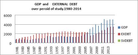
Source: the data collected from the World Bank.1980-2014.
Despite its high level, Mauritania’s debt structure remains Sold. Debt is contracted with bilateral and multilateral institutions, a stable creditor base, and mostly at concessional terms. Mauritania
And bilateral creditors account for 42 and 46 percent of total debt, respectively. Mauritania exposure to regional Arab lenders, with about 60 percent of the total portfolio, could make it vulnerable to a change in their lending policies. Its debt structure includes very limited guaranteed borrowing by SOEs and debt is contacted on fixed terms, with long maturities. Sources of risks in the debt structure relate to foreign currency exposure due to the size of the external debt ,as 95% of its debt stock is denominated in foreign currency (mainly US dollar, Kuwait Dinar, and SDR).Domestic debt remains small( about 5 percent of stock) and consists of treasury bills for budgetary and liquidity management purpose. It is, nevertheless, issued at short maturity (up to six months) with some limited rollover risks. The debt service profile remains stable and relatively benign, but a term of trade shock could hamper Mauritania’s ability to servicing its external debt.
Figure1.2: Creditor base on Mauritania, 2013
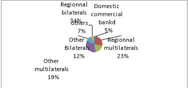
Source: Bank Central of Mauritania
1.3 HIPC debt in Sub-Saharan Africa
The main question in the 1990s was whether African counties would repay huge external debt, given the state of their economics and the macroeconomic problem that were plaguing them. Several initiatives have been developed since then. The external debt problem had major implication in Africa, the most important at the time being lack of fiscal space-reduced fiscal adjustment and a weaned ability to build capacity that could facilitate growth and external debt re-payments. For example, to support future payment ability, export supply capacity had to be improved. But this required a set of incentives, which could not be maintained in the presence of macro imbalances. Thus external debt overhand problem became a force and a major risk in Africa, preventing appropriate adjustment and reforms in the 1990. The emergence of unsustainable debt in the HIPC countries can be analyzed from both the demand and supply side. From the demand side, the group of countries which are now classified as HI-PCs needed external debt to meet their development and other needs. Most of these countries were poor with relatively lower economic growth and lower per capita income. Hence national rates of savings were also very low with domestic savings being insufficient to finance their developmental and national goals. Moreover, as most of these countries were dependent on the exports of primary commodities, their export earnings were not enough to finance import bills as they mostly imported capital intensive goods which were relatively more expensive. Hence, there arose the need for external borrowing Fortunately (or, unfortunately) due to the significant increase in the price of oil between 1973 and 1979, the foreign reserve of the oil exporting countries dramatically increased with deposited being mainly with the European banks. Thus there sprung a market for external debt or borrowing from overseas sources. During the 1970s most of the governments of the developing and poor countries heavily borrowed money primarily to finance their industrial and infrastructure development. There was a popular belief among many of the developing nations that the economic success depended on industrial development which needed protection from overseas competition during the initial stages of development. Thus industrial development was pursued with the aid of the import substitution industrialization strategy. Unfortunately, many of these countries, especially the sub-Saharan African countries failed to invest their borrowed funds in income generating activities and hence failed to enhance their ability to repay their accumulated debt. Based on the results reported in Siddique (1996), which analyses the external debt problem facing 32 sub-Saharan African nations over the period 1971 to 1990, the following three major interdependent factors were found to be contributing to the accumulation of external debt. The first is the trade policy. It is argued that governments seeking to address burgeoning external debt should pursue trade policies that would result in significantly large export earnings to meet additional debt obligations or to reduce the total stock of external debt in the long term. Otherwise, the trade policy is considered inappropriate. Siddique (1996) finds that approximately 21% of growth in the stock of external debt among the low-income countries in question was due to inappropriate trade policy for the period 1971 to 1979. The second is macroeconomic policy. Unsustainable expansionary monetary policy can result in a chronic current account deficit and fiscal imbalance leading to a build-up of external debt. Furthermore, Krueger (1987) identifies unrealistic macroeconomic policy as having the potential to induce capital flight, forcing countries to engage in further borrowing not just to meet existing debt obligations, but also to offset the impact of capital flight. Siddique (1996) identifies a number of countries during the period 1971 to 1979 for which poor macroeconomic policy was almost solely responsible for growth in net debt, but also identifies cases in which macroeconomic policy designed to achieve high economic growth enhanced the ability of debt-stricken low-income countries to meet their debt obligations. The third is external and global shocks. This accounts for the contribution to external debt from factors beyond the direct control of policymakers in low-income countries, such as real interest rates, the onset of anti-inflationary monetary policy resulting in recession, and other global economic co.nditions. Giersch (1985) identified the following three factors which contributed to the emergence of HI-PCs:
The 1973 oil price increase led to an increase in import bills of the indebted oil importing countries which led to balance of payment deficit, causing the need for adjustment of the production and consumption structures. • Interest rates remained relatively lower in the 1960s and the 1970s which prompted the developing countries to borrow more than they could afford once interest rates went up.
• The second oil shock in 1979 led to global recession in the early 1980s. Export incomes of the indebted nations shrank considerably resulting in an increase in the need for more borrowing for oil importing countries.
2 Literature Review
2.1 Review of Conceptual and Definition Issues
The act of borrowing creates debts and this debt may be domestic or external. The focus of this study is on external debt which refers to that part of a nation’s debt that is owed to creditors outside the nation. Arnone et al (2005) defines external debt as that portion of a country’s debt that is acquired from foreign sources such as l institutions. According to (Ogbeifin, 2007), external debt arises as a result of the gap between domestic savings and investment. As the gap widens, debt accumulates and this makes the country to continually borrow increasing amounts in order to stay afloat. He further defined Mauritania’s external debt as the debt owed by the public and private sectors of the Mauritanian economy to non-residents and citizens that is payable in foreign currency, goods and services.
Debt crisis occurs when a country has accumulated a huge amount of debt such that it can no longer effectively manage the debt which leads to several mishaps in the domestic political economy (Adejuwon et al). Mimiko (1997) defined debt crisis as a situation whereby a nation is severely indebted to external sources and is unable to repay the principal of the debt.
2.2 Review of Theoretical Issues
Several theoretical contributions have been made as regards the subject matter of external debt and economic growth. These theories are of relevance to this study as they serve as a building block to this research work and as such the following theories will be discussed; the dual-gap theory, debt overhang theory, crowding-out effect theory, dependency theory and the Slow-growth model
2.2.1 The Dual-gap theory
Omoruyi (2005) stated that most economies have experienced a shortfall in trying to bridge the gap between the level of savings and investment and have resorted to external borrowing in order to fill this gap. This gap provides the motive behind external debt as pointed out by (Chenery, 1966) which is to fulfill the lack of savings and investment in a nation as increases in savings and investment would vie-à-vis lead to a rise in economic growth (Hunt, 2007). The dual-gap analysis is provides a framework that shows that the development of any nation is a function of investment and that such investment requires domestic savings which is not sufficient to ensure that development take place (Oloyede, 2002). The dual-gap theory is coined from a national income accounting identity which connotes that excess investment expenditure (investment-savings gap) is equivalent to the surplus of imports over exports (foreign exchange gap).
2.2.2 External debt and Economic growth
The matter of external debt has become a major impediment to the growth and stability of developing countries. Economists have therefore chosen to explore the channels through which the effects of external debt burden are realized and have come up with two competing theories namely the debt overhang theory and the crowding-out effect theory.
Debt-overhang occurs when a nation’s debt is more than its debt repayment ability. Krugman (1982) explains debt overhang as one whereby the expected repayment amount of debt exceeds the actual amount at which it was contracted. Borensztein (1990) also defined debt overhang as one where the debtor nation benefits very little from the returns on additional investment due to huge debt service obligations. The “debt overhang effect” comes into play when accumulated debt stock discourages investors from investing in the private sector for fear of heavy tax placed on them by government. This is known as tax disincentive. The tax disincentive here implies that because of the high debt and as such huge debt service payments, it is assumed that any future income accrued to potential investors would be taxed heavily by government so as to reduce the amount of debt service and this scares off the investors thereby leading to disinvestment in the overall economy and as such a fall in the rate of growth (Ayadi and Ayadi, 2008). In addition, Clement et al (2003) stated that external debt accumulation can promote investment up to a certain point where debt overhang sets it and the willingness of investors to provide capital starts to deteriorate. Audu (2004) relates the concept of debt overhang to Nigeria’s debt situation. He stated that the debt service burden has prevented rapid growth and development and has worsened the social issues. Nigeria’s expected debt service is seen to be increasing function of her output and as such resources that are to be used for developing the economy are indirectly taxed away by foreign creditors in form of debt service payments (Ekperiware et al, 2005). This has further increased uncertainty in the Nigerian economy which discourages foreign investors and also reduces the level of private investment in the economy.
Cohen (1993) and Clement et al (2003) observe that aside from the effect of high debt stock on investment, external debt can also affect growth through accumulated debt service payments which are likely to “crowd out” investment (private or public) in the economy. The crowding-out effect refers to a situation whereby a nation’s revenue which is obtained from foreign exchange earnings is used to pay up debt service payments. This limits the resources available for use for the domestic economy as most of it is soaked up by external debt service burden which reduces the level of investment.
Tayo (1993) opined that the impact of debt servicing of growth is damaging as a result of debt-induced liquidity constraints which reduces government expenditure in the economy. These liquidity constraints arise as a result of debt service requirements which shift the focus from developing the domestic economy to repayments of the debt. Public expenditure on social infrastructure is reduced substantially and this affects the level of public investment in the economy.
Furthermore, some researchers have come up with other ways through which external debt may affect economic growth. According to (Borenstein, 1990) external debt affects growth through the credit rationing effect which is a condition faced by countries that are unable to contract new loans based on their previous inability to pay.
2.2.3 The Dependency Theory
The dependency theory seeks to outline the factors that have contributed to the development of the underdeveloped countries. This theory is based on the assumption that resources flow from a “periphery” of poor and underdeveloped states to a “core” of wealthy states thereby enriching the latter at the expense of the former. The phenomenon associated with the dependency theory is that poor states are impoverished while rich ones are enriched by the way poor states are integrated into the world system (Todaro, 2003; Amin, 1976).
Dependency theory states that the poverty of the countries in the periphery is not because they are not integrated or fully integrated into the world system as is often argued by free market economists, but because of how they are integrated into the system. From this standpoint a common school of thought is the bourgeoisie scholars. To them the state of underdevelopment and the constant dependence of less developed countries on developed countries are as a result of their domestic mishaps. They believe this issue can be explained by their lack of close integration, diffusion of capital, low level of technology, poor institutional framework, bad leadership, corruption, mismanagement, etc. (Momoh and Hundeyin, 1999). They see the under-development and dependency of the third world countries as being internally inflicted rather than externally afflicted. To this school of thought, a way out of the problem is for third world countries to seek foreign assistance in terms of aid, loan, investment, etc, and allow undisputed operations of the Multinational Corporations (MNCs). Due to the underdeveloped nature of most LDC’s, they are dependent on the developed nations for virtually everything ranging from technology, aid, technical assistance, to culture, etc. The dependent position of most underdeveloped countries has made them vulnerable to the products of the Western metropolitan countries and Breton Woods institutions (Ajayi, 2000). The dependency theory gives a detailed account of the factors responsible for the position of the developing countries and their constant and continuous reliance on external for their economic growth and development.
2.3 Theoretical of literature
The economic literature of recent times on open economies shows that reasonable levels of external borrowing by a developing country can its economic growth into capital accumulation and productivity growth. Countries at their early stages of development have small stocks of capital and are likely to have investment opportunities with higher rates of return. However, due to the low level of savings in developing countries, which reflects their low incomes, domestic savings should be supplemented by foreign resources. As long as these countries use the borrowed funds for productive investment and do not succumb to macroeconomic instability and policies that distort economic incentives, or sizable adverse economic shocks, growth should increase and allow for timely debt repayments (Pattillo, Poirson and Ricci, 2004).
Why do large levels of accumulated debt lead to lower growth? The best-known explanation comes from “debt overhang” theories, which show that, if there is some likelihood that, in the future, debt will be larger than the country’s repayment ability, expected debt-service costs will discourage further domestic and foreign investment and thus harm growth. Potential investors will fear that the more a country produces, the more it will be “taxed” by creditors to service the external debt, and thus they will be less willing to incur costs today for the sake of increased output in the future. Eduardo Borensztein (1990) also defined the debt overhang crisis as a situation in which the debtor country benefits very little from the return to any additional investment because of the debt service obligations.
The heavy debt-service payments have inevitably put great pressure on the budget, leading to rising fiscal deficits in the highly indebted countries. This leads to several problems. The first is that taxes need to be increased in order to raise the resources (in domestic currency) to service the debt. One of the consequences of the anticipated tax burden is to depress investment; second, it is necessary to transform the domestic resources in to foreign exchange, in which debt service External Debt must be paid. The desperate demand for foreign exchange to service debt often results in aid resources being routinely diverted to finance debt-service payments. Third, the stiff demand of high debt-service payments on the budget results in forced reductions in public investment and reduced spending on education and health. The diversion of resources from public investment to debt service is related to the crowding out hypothesis. Thus; growth is bound to be regarded as a result of the depressing effect on investment of heavy debt service payments and the reduction of growth supporting government’s expenditure
Debt overhang can also greatly slow down long‐run growth because it reduces government’s incentive to carry out structural and fiscal reforms, since these reforms could intensify pressures to repay foreign creditors. These disincentives for reforms are of special concern especially in low‐income countries, where an acceleration of structural reforms is needed to sustain higher growth a high level of external debt also depresses investment and growth by increasing uncertainty about actions and policies that the government will undertake in order to meet its debt servicing obligations. In particular, there may be expectations that debt service payments will be financed by deformation measures (the inflation tax, for example). In these circumstances, potential private investors will prefer instead to wait (Serven, 1997). In addition, the stock of external debt matters particularly in periods of crises. That is, when a crisis strikes, the ability of the government to intervene depends on the amount of debt that it has already accumulated as well as what its creditors perceive to be its capacity to raise tax revenues to serve and repay the debt. Public authorities may become constrained both in their attempt to engage in traditional counter-cyclical stabilization policies and in their role as lender of last resort during a financial crisis. Hence, high levels of public debt can limit essential government functions. In sum, the theoretical literature suggests that foreign borrowing has a positive impact on investment and growth up to a certain threshold level, beyond which its impact is adverse. That is, the relationship between the debt value and investment—and then growth — can be represented as a kind of “Lifer curve.
In Kurgan’s specification the external debt overhang affects economic growth through private investment, as both domestic and foreign investors are deterred from supplying further capital. Other channels may be total factor productivity, as proposed in Patillo et al. (2004), or increased uncertainty about future policy decisions, with a negative impact on investment and further on growth, as in Agénor and Montiel (1996) and in line with the literature of partly-irreversible decision making under uncertainty (Dixit and Pindyck 1994). The empirical evidence on the relationship between debt and growth is scarce and primarily focused on the role of external debt in developing countries. Among more recent studies, several find support for a non-linear impact of external debt on growth, with deleterious effects only after a certain debt-to-GDP ratio threshold. Pattillo et al (2002) use a large panel dataset of 93 developing countries over 1969-1998 and find that the impact of external debt on per-capita GDP growth is negative for net present value of debt levels above 35-40% of GDP.
There are numerous theoretical contributions have focused on the adverse impact of external debt on the economy and the circumstances under which such impact arises. In this line of research Krugman (1988) coins the term of “debt overhang” as a situation in which a country’s expected repayment ability on external debt falls below the contractual value of debt Cohen’s (1993) theoretical model posits a non-linear impact of foreign borrowing on investment (as suggested by Clements et al. (2003), this relationship can be arguably extended to growth). Thus, up to a certain threshold, foreign debt accumulation can promote investment, while beyond such a point the debt overhang will start adding negative tension on investors’ willingness to provide capital.
Cohen (1993) and Clements et al. (2003) corroborate the aforementioned impact of debt, as they observe that the negative effect of debt on growth works not only through its impact on the stock of debt, but also through the flow of service payments on debt, which are likely to ‘crowd out’ public investment. This is so because service payments and repayments on external debt soak up resources and reduce public investments. The damaging impact of debt servicing on growth is attributable to the reduction of government expenditure resulting from debt-induced liquidity constraints (Taylor, 1993). Liquidity constraint, implied by the debt-servicing requirements, may shift the budget away from the social sector or public investment. This is important for consideration because public expenditures are likely to be a major determinant of the economic activities in many functional sectors (Fosu, 2007). Accumulated debt stock reduces economic performance through ‘debt overhang’ effect (tax disincentive and macroeconomic instability). Tax disincentive means that a large debt stock discourages investments because potential investors assume that there would be taxes on future income in order to make debt repayments. The macroeconomic instability relates to increases in fiscal deficit, uncertainty due to exceptional financing, exchange rate depreciation, possible monetary expansion, and anticipated inflation (Claessens et. al. 1996). In the Ricardian view, government debt is considered equivalent to future taxes (Barrn,1974), and as noted in Sheikh, Faridi and Tariq (2010), the utility quality of the consumers, the discounted sum of future taxes is equivalent to the current deficit. So the shift between taxes and deficits does not produce aggregate wealth effects. The increase in government debt does not affect aggregate demand. The rational consumer facing current deficits saves for the future rise in tax and consequently total savings in the economy are not affected. This theory means that domestic debt has a neutral effect on the economy’s output. Sheikh, Faridi and Tariq (2010) further established that domestic debt has a positive impact on growth, inflation and saving from a well developed capital markets which enhance the volume and efficiency of private investment. They are of the view that moderate level of non inflationary domestic debt has a direct influence on economic growth enhancing private savings and strengthening financial Internationale. Inheritance and Rother (2010) empirically investigated the impact of high and growing government debt on economic growth of the Euro countries for a period which spanned between 1970 and 2009. They established that the channel through which government debt (domestic or external) influence economic growth are private savings, public investment, total factor productivity and real increase rate. The study revealed a nonlinear negative impact of government debt on economic growth Uzochukwu (2005) using per capital income approach investigated the impact of public debt and economic growth on poverty in Nigeria. The study revealed that domestic external and debt service payment have inverse impact on economic output and lead to backward reduction in poverty. Adofu and Abula (2010) investigate empirically the effect of domestic debt and economic growth in Nigeria using the Ordinary Least Square (OLS) regression technique and employing time series data from 1986 to 2005. The study revealed that domestic debt has negative effect on economic growth such that domestic debt decreases gross domestic product by 42.8 percent, and advocated that the Nigerian government should reduce domestic borrowing and improve on her Tax Structure. Bolaji, Olukayode and AddilMaliq (2010) used a disaggregated approach to determine the long-run effect of debt financing mix (that include Treasury Bill, Development stock, Treasury Certificate and Bond, Multilateral Debt Source and international lending clubs) on economic growth and development in Nigeria. The study posited that development stock and treasury certificate bond which are component of domestic debt are the best debt financing mix to propel the development of the Nigerian economy in providing gin infrastructure facilities and undertaking developmental projects that will enhance the standard of living of the citizen, as well as increase the national output and aid the achievement of other target macroeconomic objectives of the government.
2.4 Empirical of Literature
Several cross-country and country specific studies have been conducted on the relationship between external debt and economic growth using different methodologies. Some of the literature will be discussed below.
There are literature that analyze the impact of external debt on economic growth using linear regression model and arrived at positive and negative impacts of external debt on economic growth. Maureen Were (2001) for Kenya for the period 1970- 95 arrived at the negative impact of debt accumulation on economic growth and private investment but debt servicing does not appear to affect growth adversely but has some crowding-out effects on private investment. Similarly, Rifaqat Ali and Usman Mustafa (2013) for Pakistan for the period 1970-2010 found that external debt exerts significant negative impact on economic growth. This confirmed the existences of debt overhang problem for Kenya and Pakistan. On the other hand, the study on Nigeria by OKE Michael O. et al (2012) for the period 1980 to 2008 indicates that there exists a positive relationship between external debt, economic growth and investment. Similarly, Faraji Kasidi (2013) for the period of 1990-2010 for Tanzania and Hasan Shah. M ET AL (2012) for the case of Bangladesh during the period 1974 – 2010 concluded that there is a positive effect of total external debt stock on GDP growth while the debt service payment has a negative effect on growth.The empirical and analytic studies in 1990s were unanimous that the magnitude of external debt problem in Africa was shackling its growth and investment(see e.g Elbadawi,Ndulu,and Ndung’u 1997;Ndung;u 2003;Clements, Bhattachary, and Nguyen2003).The debt burden significantly threatened Africa’s hope of future economic growth recovery. Drastic action was needed to help these countries out of the conundrum.
The empirical evidence on the relationship between debt and growth is scarce and primarily focused on the role of external debt in developing countries. Among more recent studies, several find support for a non-linear impact of external debt on growth, with deleterious effects only after a certain debt-to-GDP ratio threshold.
On the empirical level, several studies are unanimous that debt overhang is a major reason for slowing economic growth in indebted countries. They posit that heavy debt burdens prevent countries from investing in their productive capacity, investment necessary to spur economic growth. Disincentives to investment also arise for reasons largely related to investor’s expectations about the economic policies required to service debts.
3 The methodology of this research
3.1 specification of the model
Following a debt-growth model adopted by Elbadawi (1996) for developing countries and used by were (2001) for Kenya and Frimpong .J.M et AL (2006) for Ghana a debt-growth equation for Ethiopia is estimated. It is well known that the expansion of investment facilitates economic growth, depending on the quality of investment. Consequently, it is important to evaluate the impact of external indebtedness on investment. However debt can also affect economic growth directly through its effects on the productivity of investment. External debt may still affect output growth even if investment levels remain unaffected. As the stock of debt and cost of external debt servicing rise, there is little left to finance public projects that leads to fiscal deficits that further aggravate external borrowing. As a result, the VECM model is used as the major variables are suspected to affect one another through different channels. Of course, there are a number of variables that affects GDP growth that have not been included in the specification, such as aid, labor force, export and import, CPI, rainfall etc., as the purpose of the study is not to look at determinants of real GDP. The vector of the VECM model, therefore, incorporates only four variables- Real GDP (Y), external debt (ED), debt service (DS) and investment (I).This study objective is to estimate the impact of the External Debt(ED) through GDP on Mauritania .Thus, ECM is as follows:
∆F=γ+∑i=1sδi∆Fi-1+∑j=1Fαj∆Zt-1+θECTt-1 +∂t
ECT(t-1) are the lagged stationary residuals from the co-integration equations, Ft is the dependent variable Z is a vector of independent variables,
γis the regression intercept,
αj and
δiI are the coefficients of variables and
θis the coefficient of the error correction term .
3. 2 Techniques of Estimation
The research applied the unit root, co-integration and error correction modeling .This is to discover the order of integration of the variables in the study to avoid spurious empiric
Cal results. Methodologically, the co-integration procedure demands that we control unit root test before co-integration and ECM estimation. We used the Dickey Fuller and the Augmented Dickey Fuller tests. The employment variable notes that a time series is non-stationary if the mean and variance of time series is depend over time. On the other way, a time series is expressed as stationary if the mean and variance is constant over time. Experimental, most economic time series are non-stationary and only achieved stationary at the first difference level or at a higher level.
Time series data covering a period of 34years will be estimated using Co-integration technique of analysis which is an improvement on the classical ordinary least square technique (OLS). This technique was chosen as it depicts long-run economic growth. The following techniques of estimation are employed in carrying out the co-integration analysis:
3.2.1 Unit Root Test
This is the pre Co-integration test. It is used to determine the order of integration of a variable that is how many times it has to be difference or not to become stationary. It is to check for the presence of a unit roots in the variable i.e. whether the variable is stationary or not. The null hypothesis is that there is no unit root. This test is carried out using the Augmented Dickey Fuller (ADF) technique of estimation. The rule is that if the ADF test statistic is greater than the 5 percent (critical value ) we accept the null hypothesis i.e. the variable is stationary but if the ADF test statistic is less than the 5 percent critical value i.e. the variable is non-stationary we reject the null hypothesis and go ahead to difference once. If the variable does not become stationary at first difference we difference twice. However it is expected that the variable becomes stationary at first difference. The test procedure is that the variable has a unit root or at bets is non-stationary when &=1.However,if the variable should become stationary after differencing, then it is integrated of order D, where D is the number of times it was adherence before becoming stationary.
3.2.2 Co-integration test
Co-integration is one of the key concepts of modern economics. Let’s start by giving an intuitive explanation and its properties. Two or more processes are said to be co-integration if they stay close to each other even if they “drift about” as individual processes. A colorful illustration is that of the drunken man and his dog: both stumble about aimlessly but never drift too far apart. Co-integration is an important concept both for economics and financial modeling. It implements the notion that there are feed-backs that keep variables mutually aligned.
Co-integrated processes are characterized by a short-term dynamics and a long-run equilibrium. Not that this latter property does not mean that co integrated processes tend to a long-term equilibrium. On the contrary, the relative behavior is stationary. Long-run equilibrium is the static regression function, that is, the relation between the processes after eliminating the short-term dynamics.
3.2.3 Vector Error Correction Model
The method developed by Johansen (1988) is undoubtedly the most widely used method in applied work. Models using this approach are known as vector error correction (VECM) or co-integration var (CIVAR) models. VECM can be seen as scaled down VAR model in which the structure coefficients are identified
The justification for the VECM approach is that identification and testing for the significance of the structural coefficients, underlying the theoretical relationships, is important. The simple VAR models do not identify structural coefficients nor do they take seriously the relevance of unit tests.
The Vector Error Correction Model (VECM) shows the speed of adjustment from short-run to long run equilibrium. The a prior expectation is that the VECM coefficient must be negative and significant for errors to be corrected in the long run.
Without giving the full details of the estimation can be summarized as follows. Virtually
3.2.4 G ranger Causality test
This is used to check for causality between two variables. In this case our aim is to test for a causal relationship between external debt and economic growth. The rule states that if the probability value is between 0 and 0.05 there is a causal relationship
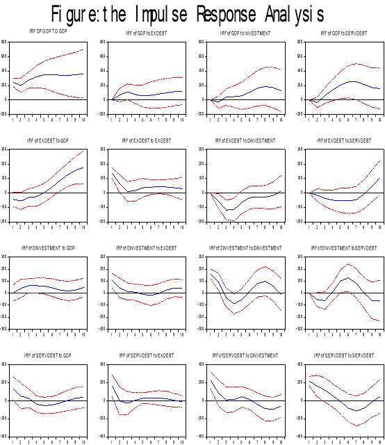
3.2.5 Impulse Response Analysis
The impulse response function is one of the most important useful outputs VECM from analysis.
The result of the analysis shows how the variables reaction to each other. The section we will focus on the response of GDP to one S.D shocks to the other variable on the model.
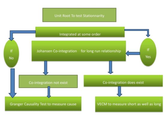
This figure below shows the important steps we should to do to run the Vector error correction model.
The figure show the important steps to rum off Vector error correction model

3.3 The hypotheses to be tested in the course of this study include
HYPOTHESIS 1
H0: There is no significant long run relationship between external debt and economic growth in Mauritania.
H1: There is a significant long run relationship between external debt and economic growth in Mauritanian.
HYPOTHESIS 2
H0: There is no causal relationship between external debt and economic growth in Mauritania.
H1: There is a causal relationship between external debt and economic growth in Mauritania.
For the first hypothesis, we have the null hypothesis which supposes that is no significant long-run relationship between external debt and economic growth in Mauritania. Beside the null hypothesis, we have the alternative hypothesis which supposes that there is a significant long run relationship between the external debt and economic growth in Mauritania. To test this hypothesis we use the result of the Vector error correction model and co-integration test.
The second hypothesis makes to test whether there is causality between the External debt and economic growth in Mauritania. The null hypothesis supposes that there is no causality between the two variables on the model. The alternative hypothesis supposes that there is causality between the two variables. To test this hypothesis we going to use G ranger Causality test using E views.
4 Data analysis & interpretation
4.1 introduction
This Thesis seeks to examine the impact of external debt on economic growth in Mauritania. This chapter therefore comprises of the data presentation, estimation and results of the empirical investigation carried out .it also addresses the relationship between external debt and economic growth in Mauritania in the long run. This chapter is further divided into trend analysis which shows the trend of time series data used from 1980-2014, descriptive analysis which contains the measures of central tendency which include mean, mode, median as well as measures of variation and other statistical characteristics of the variables and econometric analysis of co-integration Error correlation models, the G ranger Causality test and then the impulse response. This chapter distribute with the analysis of data and the interpretation of results. to avoid misleading results, econometric theory requires that variables are stationary before the application of standard econometric techniques. This is because, time series data are assumed to be non stationary and the results obtained from the OLS method may be spurious.
4.2 Data Source and Description of variables
This study uses time series data from 1980to 2014. Other periods were not covered in this study due to data problem for external debt and debt service variables. The data used in this study is from the Bank World and The Bureau National of Statistic of Mauritania . The variables entered the model are described as follows:
GDP: is the Gross domestic product of Mauritania
External Debt (EXDDEBT): is the total outstanding debt of the country. Theoretically, external debt is expected to be either positively or negatively related with economic growth depending on the usage of such external debt.
Debt Service (SERVDEBT): is payment against loan. It includes interest and principal payments. As debt servicing is a resource drain exercise it is expected to be negatively related with economic growth.
Investment : is the gross capital formation of a country.
4.3 Descriptive analysis
Table 4.1 Summary Statistics:
| Measures | GDP | EXDEBT | INVESTMENT | SERVDEBT |
| Mean | 1988.600 | 2153.343 | 171.3143 | 426.3744 |
| Median | 1402.000 | 2259.000 | 15.00000 | 297.1920 |
| Median | 1402.000 | 2259.000 | 15.00000 | 297.1920 |
| Median | 1402.000 | 2259.000 | 15.00000 | 297.1920 |
| Std. Deb. | 1457.722 | 627.5561 | 333.4034 | 415.6204 |
| Skewness | 1.166273 | 0.049993 | 2.377876 | 2.064828 |
| Kurtosis | 2.846915 | 3.263242 | 7.939602 | 6.081438 |
| Jarque-Bera | 7.968630 | 0.115636 | 68.56625 | 38.71775 |
| Probability | 0.018605 | 0.943822 | 0.000000 | 0.000000 |
| Sum | 69601.00 | 75367.00 | 5996.000 | 14923.10 |
| Sum Sq. Dev. | 72248406 | 13390108 | 3779366. | 5873170. |
| Observations | 35 | 35 | 35 | 35 |
Mean is the average Value of the series which is gotten by dividing the total value of series by the number of observations. From the above table we see the mean GDP(Gross Domestic Product), EXTDEBT(EXTERNAL DEBT), DINVEST(DIRECT INVESTMENT) AND SOD(SERVICES OF DEBT) are 3131.486,2153.343,171.3143 and 426.3744 respectively.
Median is the middle value of the series when the values are arranged in an ascending order. From the table the median for GDP, EXTDEBT, DINVESTMENT and SOD are 1402, 2259, 15 and 297. 1920 respectively.
Maximum and minimum are the maximum and minimum values of the series in the current sample. The maximum and minimum values for GDP, EXTDEBT, DINVESTMENT and SOD is 44031&683,839&627.5561,-3&333.4034 and 1703.520&119.7760 respectively.
Standard deviation is a measure of spread or dispersion in the series. From table the standard deviation for GDP, EXTDEBT, DINVESTMENT and SOD is 7255.683,627 .5561.333 and 4034,415 respectively.
Skewness is a measure of asymmetry of the distribution of the series around its mean. The Skewness of a normal distribution is zero .Positive Skewness implies that the distribution has a long right tail and negative means that the distribution has a long left tail.From the table above table. From the above table all the variables have long right tails.
4.4 Vector Error Correction Estimates test
4.4.1 log selection:
The researcher used a 4-varible VAR model to choose lag length. The optimum lag lengths of vector auto regressions(VARs)were tested using the Akaike Information Criteria (AIC), Hannan–Quinn information criterion (HQ), Schwarz information criterion (SIC), Final prediction error (FPE) and Sequential modified LR test statistic (LR).the five criterions select slag length 3 The Schwartz information Criterion selected lag and the LR method indicate lag 3.This indicates that there3 lag selected by the criteria..
Table4.3 below shows the result of VAR order selection Criteria. .
| Lag | LR | FPE | AIC | SC | HQ |
| 0 | NA | 1.73e+13 | 36.15568 | 36.24729 | 36.18604 |
| 1 | 58.15749 | 2.99e+12 | 34.40025 | 34.67507 | 34.49134 |
| 2 | 4.491617 | 3.26e+12 | 34.48389 | 34.94193 | 34.63572 |
| 3 | 19.3521* | 1.5e+12* | 33.9572* | 34.6098* | 34.228* |
*indicated log order selected by the criterion.
LR: Sequential modified LR test statistic (each test at 5% level).
AIC: Akaike information error. SC: Schwarz information criterion .
HQ: Hannan-Quin information Criterion. FPE: Final Prediction error.
4.4.2-Test of co-integration
The co-integration have a precondition that is variables must be non-stationary at level but when we convert all the variables into first difference they will become stationary ,that mean the variables should be integrated of some order. To find if the variables are non-stationary at the first difference we can use servile tests. We chose unit root to do it.
Unit Root test result
This test accomplish by using the Augmented Dickey Fuller (ADF) test, this test is relating on model with constant and trend. . The null hypothesis states that the variables has Unit Root (No stationary).as we know we reject the H0when the Statistic Value is great than Critical Value. From the table below at the first different we can see that the trace statistics is big then critical value therefore the variables is stationary at the first difference. From the table below we can see, at level the variables are non-stationary .but as the first difference; the all variables are stationary at 5% significance level. We can also know the all variables doesn’t stationary at level I (1)
Table 4.4Unit root test using Augmented Dicey-Fuller (Stationnarity Test Results).
| Variables | ADF Test statistics | ADF Critical Values* | Remarks |
| GDP | -6.603 | -2.95 | I(1) .S |
| External debt | -4.3013 | -2.95 | I(1).S |
| Investment | -5.94 | -2.95 | I(1)S |
| Service of debt | -7.13 | -2.96 | I(1).S |
| Note:* indicates critical values at 5% level of significant. | |||
Regarding the results of the unit root, the tests above confirm the non-stationery of the variables in the Var, we can then apply Johansen methodologies for co-integration.
To determine the number of co-integration vectors ,we analysis the result on the table below .for the first three null hypothesis we can see that Trace statistic is greater than the critical value so we can not accept the null hypothesis which are non,at most1,at most 2 co-integration ,rut-her we accept the alternative hypothesis.For the null hypothesis(At most 3 co-integration) , the trace statistic is less then the critical value so we can not reject the null hypothesis.Therefore the result shows that in our model there are 3 concentration at 5% level of confidence. Thereby confirming existence of long run equilibrium relationship between economic explanatory variables.
Table 4.5 the result of co-integration test is show on this table below
| Hypothesized | Eigenvalue | Trace Statistic | Critical Value 5% | Prob |
| None* | 0.636956 | 69.79 | 47.48 | 0.001 |
| At most1* | 0.4983 | 39.4 | 29.79 | 0.003 |
| At most2* | 0.4225 | 18.7 | 15.49 | 0.016 |
| At most 3* | 0.071 | 2.22 | 3.84 | 0.136 |
5 Conclusion and recommendation
The thrust of this Study has been to ascertain empirically the impact of External debt on gross domestic product (GDP) in Mauritania. The major finding obtained in the study is that external debt effect on gross domestic product is significant and positive in Mauritania. Moreover, the result indicates that a service of debt has significant and positive effect on GDP in Mauritania. However, the study concluded that growth in investment does not result in the growth of GDP. The VECM result shows that there are a long-run relationship between external debt, debt services and GDP in Mauritania. The Gander causality test demonstrates that there are uni-direction causality between External debt and Gross domestic product.
However this result seems to contradict to Mauritania’s economic situation, where External debt grew without any amelioration in the GDP. The more visible explanation of this is that Mauritania lacks sound infrastructures and suffers from poor institution yet having large stock of debt. Another possible reason is that because of management of the debt’s funds is not always channeled to the real productive sectors, mismatching of the funds and/or diversion of the funds to private hands.
This empirical analysis shows that External debt discourages investment.
It is also observed that External debt has a positive impact on economic growth in Mauritania, but this does not mean that the government should continue to increase foreign debt, because this would depend on external obligatory and, the owners of the debts may be subject to the economic policy of the convicted countries.
Debt service is a burden on the rate of the economy that may be because of the conditions under which the debts were taken .Therefore; the government must consider these conditions to re-structure them to serve the policy followed.
The external debt should be taken only for economic reasons and not for social or political reason. This can avoid the country the accumulation of External debt.
Reference
- Public Debt and the limits of fiscal to increase Economic Growth.Vladimir K. Tales .Caio Cesar Mussolini . 25 November 2013.
- Public debt and Growth : Heterogeneity and non-linearity. Mark’s Eberhardt, F.Presbitero . Journal of international Economics.2015
- External debt and economic growth in Tunisia. Nasfi Fkili Wahiba .Doctor of Economics Research unit “Enterprise Economy Environment” Higher institute of Management .Vol IV, 6 December 2014.
- The impact of External debt on Economic growth; Empirical Evidence from highly Indebted Poor Countries. By Abu Siddique, University of Western Australia .27march 2015.
- Effect of External Debt on Economic Growth and development of Nigeria. By AJAYI.LAWRENCE, BOBOYE.PH.D. vol3 No012 June 2012
- Government Debt and Economics growth in India. Anrudha, Barik.PH.D Jawaharlol Nehru University. New Delhi. Jel Code:E22,H63.040
- The impact of External debt on Economic Growth: A Comparative Study of Nigeria and South Africa.Folorinso S.Ayadi. University of Lagos.
- Assessing the Short and Long run Real Effect of Public External debt .The case of Tunisia. Ben Mimoun Mohamed. African Development Review .Vol25 No4.2013.587-606
- Debt sustainability Analysis on Mauritania .Approved by Alan Masarthur and Dhaneshwav Ghava (IMF). 26February 2012
- Nigeria’s External debt and Economic growth: An error correction Approach. Vincent N.Ezeabasili PhD. Department of Capital Market and studies .Anmba State university, Lgbriam Campus Nigeria .Vol6 No5 may 2011.
- Audu, Isa (2004). “The Impact of External Debt on Economic Growth and Public Investment: The Case of Nigeria”. African Institute for Economic Development and Planning (IDEP) Dakar Senegal. http://www.unidep.org.
- David UMORE ,”Employment and International Trade Flows in Nigeria: VECM Analysis” Department of Economics, Banking &Finance, Faculty of Social & Management Sciences ,Benson Idahosa University ,Benin City,Nigeria.Vol.8,2013.
- B.Bhaskara Rao.”Estimating Short and Long Relationships: A Guide to the Applied Economist. University of the South Pacific, Suva (Fiji).Methodological Issues May-2005.
- Muhammad Kazim Jafri. Impact of External Debt Service Payment on Investment of PAKISTAN. Pakistan Institute of Labor Education and Research ,Karachi.Proceedings of 2nd International Conference on Business Management(ISBN:(978-969-9368-06-6)
- Michael Hauser ”Vector error correction model, VECM Co integrated VAR. WS 16/17
- Genet Abera “An Empirical Analysis of External Debt and Economic Growth in Ethiopia :A Vector Auto Regressive(VAR) Approach, March 2016
- Talknice Saungweme and Shylet Mufangdaedza “An Empirical analysis of the Effects External debt on poverty in Zimbabwe:1980-2011”Great Zimbabwe University, Box 1235,Masingo,Zimbabwe
- Yan Rue Wu. “Local Government debt and Economic Growth in China”. Economics Business School. University of Western, Australia. China Economic Research Institute at the Stockholm School of Economics and National School of Development at Peking University Stockholm 28-29 August 2014
Appendix
Appendix A: vector error correction model test result
| Coefficient | Std. Error | t-Statistic | Prob. | |
| C(1) | -0.312549 | 0.157956 | -1.978708 | 0.0760 |
| C(2) | 0.150779 | 0.166969 | 0.903037 | 0.3877 |
| C(3) | 3.107560 | 1.391877 | 2.232640 | 0.0496 |
| C(4) | 0.261301 | 0.273433 | 0.955630 | 0.3618 |
| C(5) | 0.059746 | 0.239083 | 0.249895 | 0.8077 |
| C(6) | -0.021422 | 0.216494 | -0.098950 | 0.9231 |
| C(7) | 0.240823 | 0.171620 | 1.403239 | 0.1908 |
| C(8) | 0.242563 | 0.279083 | 0.869143 | 0.4051 |
| C(9) | -0.119960 | 0.247287 | -0.485103 | 0.6381 |
| C(10) | -0.290416 | 0.308812 | -0.940430 | 0.3692 |
| C(11) | 0.538166 | 0.294934 | 1.824697 | 0.0980 |
| C(12) | -2.851542 | 1.287856 | -2.214178 | 0.0512 |
| C(13) | -2.559054 | 1.055484 | -2.424532 | 0.0358 |
| C(14) | -2.087955 | 1.225151 | -1.704243 | 0.1192 |
| C(15) | -4.066994 | 1.624344 | -2.503777 | 0.0312 |
| C(16) | -0.073587 | 0.368140 | -0.199888 | 0.8456 |
| C(17) | -0.503316 | 0.384578 | -1.308748 | 0.2199 |
| C(18) | 0.268605 | 0.323007 | 0.831575 | 0.4251 |
| C(19) | 0.634767 | 0.346593 | 1.831450 | 0.0969 |
| C(20) | 326.4740 | 118.5268 | 2.754433 | 0.0203 |
| R-squared | 0.948598 | Mean dependent var | 144.4667 | |
| Adjusted R-squared | 0.850936 | S.D. dependent var | 295.6759 | |
| S.E. of regression | 114.1571 | Akaike info criterion | 12.54775 | |
| Sum squared reside. | 130318.4 | Schwarz criterion | 13.48188 | |
| Log likelihood | -168.2162 | Hannan-Quinn criter. | 12.84659 | |
| F-statistic | 9.712988 | Durbin-Watson stat | 2.865688 | |
| Prob(F-statistic) | 0.000400 | |||
Appendix B: Wald Test
| Null Hypothesis | Test Statistic | Value | Critical value 5% | Prob |
| C1 =C2=0 | F-Statistic | 0.47* | 2.1 | 0.6 |
| C3=C4=0 | F-Statistic | 3.02** | 2.1 | 0.09 |
| C5=C6=0 | F-Statistic | 6.84** | 2.1 | 0.001 |
Noted: c1, c2 is the coefficient of External debt on two lag. c3, c4 is the coefficient of Investment on two lag period .c5; c6is the coefficient of service debt. * noted accept the null hypothesis. ** noted as reject the null hypothesis.
Appendix C: Co integration test result
| Unrestricted Cointegration Rank Test (Trace) | ||||
| Hypothesized | Trace | 0.05 | ||
| No. of CE(s) | Eigenvalue | Statistic | Critical Value | Prob.** |
| None * | 0.636956 | 69.78906 | 47.85613 | 0.0001 |
| At most 1 * | 0.498335 | 39.39209 | 29.79707 | 0.0029 |
| At most 2 * | 0.422538 | 18.69739 | 15.49471 | 0.0159 |
| At most 3 | 0.071452 | 2.224002 | 3.841466 | 0.1359 |
| Trace test indicates 3 co integrating eon(s) at the 0.05 level | ||||
| * denotes rejection of the hypothesis at the 0.05 level | ||||
| **Mackinnon-Haug-Michelis (1999) p-values | ||||
| Unrestricted Cointegration Rank Test (Maximum Eigenvalue) | ||||
| Hypothesized | Max-Eigen | 0.05 | ||
| No. of CE(s) | Eigenvalue | Statistic | Critical Value | Prob.** |
| None * | 0.636956 | 30.39697 | 27.58434 | 0.0212 |
| At most 1 | 0.498335 | 20.69471 | 21.13162 | 0.0574 |
| At most 2 * | 0.422538 | 16.47338 | 14.26460 | 0.0220 |
| At most 3 | 0.071452 | 2.224002 | 3.841466 | 0.1359 |
Cite This Work
To export a reference to this article please select a referencing stye below:
Related Services
View all


Related Content
All TagsContent relating to: "International Studies"
International Studies relates to the studying of economics, politics, culture, and other aspects of life on an international scale. International Studies allows you to develop an understanding of international relations and gives you an insight into global issues.
Related Articles

DMCA / Removal Request
If you are the original writer of this dissertation and no longer wish to have your work published on the UKDiss.com website then please: