Slope Angle Influence in the Economic Value of an Open Pit Project
Info: 12727 words (51 pages) Dissertation
Published: 9th Dec 2019
Tagged: EconomicsEnvironmental Studies
ABSTRACT
“Knowledge has to be improved, challenged, and increased constantly, or it vanishes.”
– Peter F. Drucker
TABLE OF CONTENT
1.3.2 MINERAL RESOURCES DISTRIBUTION
2.2 MINERAL RESERVE EXTRACTION STRATEGY
2.2.1 PRELIMINARY PIT SEQUENCE ANALYSIS
2.3 MINING PRODUCTION RATE ANALYSIS
2.3.1 MINE CAPACITY AT 26Mt PER YEAR
2.3.2 MINE CAPACITY AT 30Mt PER YEAR
2.3.3 MINE CAPACITY AT 33Mt PER YEAR
2.4 MINING PRODUCTION SCHEDULE
2.5 FINAL PIT SELECCION – BASE CASE
3.2.1 MINE PRODUCTION STRATEGY
3.2.2 MINERAL RESERVE EXTRACTION STRATEGY
3.2.3 PRODUCTION SCHEDULE FOR SELECTED ALTERNATIVES
3.3 FINAL PIT SELECTION – STUDY CASE
4 MINING EQUIPMENT FLEET ESTIMATION
4.5 AUXILIARY AND SUPPORT EQUIPMENT
6 CONCLUSIONS AND RECOMMENDATIONS
APPENDIX A. Whittle® and Milawa Algorithm®
LIST OF FIGURES
Figure 1. Project Mineral Resource Distribution…………………………
Figure 2. Project Grade-Tonnage Curve
Figure 3. Project Cut-off Grade Equation and Calculation…………………..
Figure 4. Base Case Definition Flowsheet…………………………….
Figure 5. Pit by Pit Graph at 26Mt per year……………………………
Figure 6. Pit by Pit Graph at 30Mt per year……………………………
Figure 7. Pit by Pit Graph at 33Mt per year……………………………
Figure 8. Mine Production Schedule at 26Mt per year Mining Production Rate……..
Figure 9. Mine Production Schedule at 30Mt per year Mining Production Rate……..
Figure 10. Mine Production Schedule at 33Mt per year Mining Production Rate…….
Figure 11. Mine Production Schedule at 30Mt per year – Final Pit Selected……….
Figure 12. NPV Trend for Slope Angle Combinations……………………..
Figure 13. Pit by Pit Graph at 30Mt per year – Alternative A: W46-M48………….
Figure 14. Pit by Pit Graph at 30Mt per year – Alternative A: W46-M49………….
Figure 15. Mine Production Schedule – Alternative A: W46-M48………………
Figure 16. Mine Production Schedule – Alternative B: W46-M49………………
Figure 17. Mine Production Schedule – Study Case: W48-M49 – Final Pit Selected….
Figure 18. Shovels’ Distribution…………………………………..
Figure 19. Trucks’ Distribution……………………………………
Figure 20. Net Revenue Distribution per Case………………………….
Figure 21. Operating Expenses Distribution per Case…………………….
Figure 22. Cash Cost Distribution per Case……………………………
Figure 23. Cumulative Discounted Cash Flow Comparison…………………
Figure 24. FCF per Period and Cumulative DCF – Base Case……………….
Figure 25. FCF per Period and Cumulative DCF – Study Case……………….
Figure 26. Sensitivity Analysis – Base Case……………………………
Figure 27. Sensitivity Analysis – Study Case…………………………..
LIST OF TABLES
Table 1. Block Model Information
Table 2. Mineral Resources Distribution and Copper Grade
Table 3. Cu Grade – Descriptive Statistic Parameters
Table 4. Slope Angles Restrictions by Zone
Table 5. Project Economic Restrictions
Table 6. Nested Pit Sequence Selected
Table 7. Mining Production Rate and Selected Nested Pit Summary
Table 8. Final Pit Selection Options for Base Case
Table 9. Angle Combinations to Evaluation
Table 10. Selected Nested Pit for Alternatives
Table 11. Final Pit Selection Options for Study Case
Table 12. Result Analysis Comparison Base Case (W44-M48) – Study Case (W46-M49)
Table 13. Drilling Equipment Operational Parameters
Table 14. Loading Productivity Estimate
Table 15. Hauling Parameters by Case
Table 16. Hauling Distance Summary by Case
Table 17. Hauling Equipment Operational Parameters
Table 19. Cycle Time and Hauling Fleet Calculation Summary
Table 20. Auxiliary and Support Equipment Requirement
Table 21. Final Product Shipping Cost
Table 22. Net Revenues – Base Case
Table 23. Net Revenues – Study Case
Table 24. Net Revenue Comparison
Table 25. Operating Expenses Comparison
Table 26. Operating Expenses – Base Case
Table 27. Operating Expenses – Study Case
Table 28. Cash Cost Comparison
Table 29. Cash Cost – Base Case
Table 30. Cash Cost – Study Case
Table 31. Detail of General and Administration Costs
Table 33. Cash Flow per Period – Base Case
Table 34. Cash Flow per Period – Study Case
Table 35. Comparison of Economic Valuation Results
Table 36. Parameter Variation for Sensitivity Analysis
Table 37. Sensitivity Analysis Results – Base Case
1.1 PROJECT BACKGROUND
According to USGS[1], “As large emerging economies, such as China and India, increase their participation in the global economy, demand for critical mineral resources is increasing at a rapid rate (Cunningham, 2008)”, and it implies a challenge for regions dependable of the extraction of mineral materials as a main source of incomes.
Several countries rely on mining industry a large part of its GPD, investment, employment, and direct and indirect services, which at ends has supported the country development and inhabitants’ living standards. But mining industry, like virtually all industrial activity, aims to deliver an economic return to their shareholders by the risk they have taken. However, mining industry differs from any other industrial activities, highlighting its finite duration, static condition in geographical terms, intensive in capital and prolonged periods of investment and construction with high-risk levels, the latter mainly influenced by variations of market conditions and geological uncertainty of mineral deposits.
Also, every mining project is constituted by a series of stages, which in sequence, allow the business materialization: prospecting and exploration (delimitation of the deposit in terms of mineral and economic limits), development (technical-economic analysis of the mining method and construction), mining (extraction of interest mineral resources), processing (transformation of resources extracted into tradable goods) and finally, reclamation (restoring of ecosystems to their original conditions, prior to the start-up of the project).
One of the key processes for the success of a mining project is mining design and planning, where extractable reserves are defined and established, and technical parameters of construction that optimize extraction, production capacities and mine life are set.
In this context, the selection of the overall slope angle is a critical decision in an open pit design, which might have far-reaching effects on cash flow and overall profitability in a mining project. Given its importance, this Engineering Report is based on analyzing the influence of this design parameter on the execution of an open pit mine and its final economic impact on the business, seeking the maximization of the asset value.
The Company[2] is developing a copper Project2 placed in a porphyry copper zone in the Northern Chile2. The Project is underneath 50m a waste rock layer and owns an average copper grade of 0.07%.
Currently, the Project is considering a final pit design with 44 and 48 degrees slope angle for the waste rock zone (Z-1) and mineralized zone (Z-2), respectively. This Engineering Project is looking for the maximization of the Project value by varying these angles, limited for geotechnical restrictions, seeking the best combination of them and evaluating them from a technical and economic viewpoint.
The theory behind this approach is that the deepest is the operation or the highest is the slope angle in an open pit mine, the fastest is the extraction of reserves and the best is the economic result. However, the wall stability in the pit cannot be neglected, focus special attention in safety of personnel and equipment, and integrity of the pit to ensure a continuous operation during the life of the mine project (Contreras, 2005).
1.2 PROJECT OBJECTIVES
The main purpose of this study is determining the best combination of slope angles that maximize the profitability and feasibility of the Project.
To achieve this objective is required to conduct previous analyses, or define secondary objectives, as follow:
- Defining a Base Case: Using the initial conditions of design, is necessary find a suitable Project’s annual mining rate.
- Analyze the influence of the slope angle variation: Once reached the optimal annual mining rate for the Project, it will be needing to analyze whether a different slope angle may increase or not the economic outcomes and select the best Study Case analyzed.
- Compare Base Case and Study Case: in order to propose a better alternative for a functional operation, a technical-economical comparison will be conducted between the Base Case and the selected Study Case to state the viability of this study.
1.3 BASE INFORMATION
1.3.1 BLOCK MODEL VALIDATION
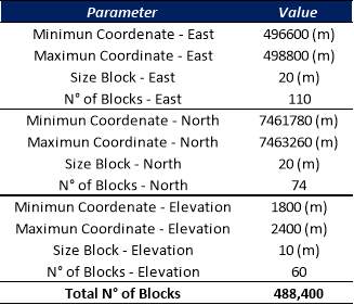
The Company has provided the basic information in a block model of the Project, updated as 2015, which hold the information shown in Table 1 (Company, 2015).
Table 1. Block Model Information
Source: Elaborated by the author, 2018
The block model contains information of block, such as Coordinate Centroid at X, Y, and Z; Resource Category (1: Measured, 2: Indicated, 3: Inferred); Copper Grade (%CuT); Mining Recovery (%); and, Density (Specific Gravity: t/m3).
To validate the model, and thus obtain certain result when processing the information, the inconsistent values of Resource Category, Copper Grade, Mining Recovery and Density (-1: no information or incoherent, like air blocks) need to be replaced by modified values (0 instead of -1).
1.3.2 MINERAL RESOURCES DISTRIBUTION
At Figure 1 and Table 2 is represented the distribution of Mineral Resources regarding its category, as Measured, Indicated and Inferred. This information was collected from the block model.
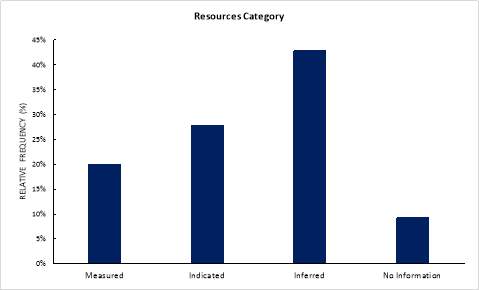
Figure 1. Project Mineral Resource Distribution
Source: Elaborated by the author, 2018
From the chart at Figure 1, is observed a great grade of confidence and certainty in Mineral Resources distribution for future analysis and more exhaustive studies due a 20% of them are Measured, 27.9% are Indicated and 42.9% are Inferred. The remaining 9.2% are blocks with no information.
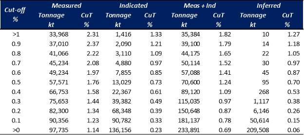
Table 2. Mineral Resources Distribution and Copper Grade
Source: Elaborated by the author, 2018
From Table 2 showing the distribution of copper grade and tonnage regarding a specific cut-off grade, is possible to visualize the average copper grade for each resource category, which fluctuates between 0.06% CuT for Inferred Resources to 1.14% CuT for Measured Resources.
1.3.3 COPPER GRADE STATISTIC
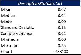
A descriptive statistic of the block model information of the Project has been made, showing the parameters of copper grade (%CuT) at Table 3, with a mean of 0.07%, a minimum grade of 0.00% and a maximum grade of 3.25%.
More information about this descriptive statistic presents a sample standard deviation and variance of 0.13% and 0.02%, respectively. These parameters indicate a uniformity in the values regarding the arithmetic mean.
Table 3. Cu Grade – Descriptive Statistic Parameters
Source: Elaborated by the author, 2018
1.3.4 GRADE-TONNAGE CURVE
At Figure 2 is presented the Project Grade-Tonnage curve, where is possible to observe that at a cut-off grade of 0.26%CuT, there are an approximately 230.6Mt of mineral resources (or 4.77% of the total tonnage of mineral resources) with an average grade of 0.76%CuT.
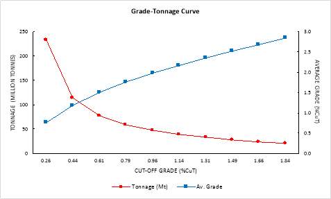
Figure 2. Project Grade-Tonnage Curve
Source: Elaborated by the author, 2018
1.3.5 CONSTRAINTS
As part of the limitations to perform this study and make the Project feasible to develop, the Company has informed the following restrictions based on previous studies:
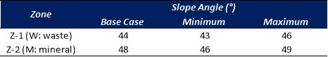
GEOTECHNICAL RESTRICTIONS
An internal report issued by the Company’s Geotechnical Studies Superintendence, limits the design parameters by establishing the minimum and maximum slope angles for Z-1 (waste rock material; above 2,280m elevation) and Z-2 (mineralized material; below 2,280m elevation) (SRK Consulting, 2015). These geotechnical restrictions, for each zone, are shown in Table 4.
Table 4. Slope Angles Restrictions by Zone
Source: Elaborated by the author, 2018
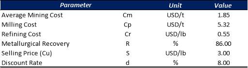
ECONOMIC PARAMETERS
The economic parameters that will be used to evaluate this Project were delivered by the Company and are based in long-term projections and benchmarking analysis, both for mining and processing operations. Table 5 shows these parameters as follow:
Table 5. Project Economic Restrictions
Source: Elaborated by the author, 2018
BREAKEVEN (MINING) COPPER CUT-OFF GRADE
For a mineral or metal to be economically mined (and therefore considered Mineral Reserve), is required calculate the Project copper cut-off grade. In this case, the economic parameters were used, and Figure 3 shows the calculation made, obtaining a cut-off grade of 0.154%CuT.

Figure 3. Project Cut-off Grade Equation and Calculation
Source: Elaborated by the author, 2018
1.4 CHAPTER SUMMARY
This chapter summarizes the base information due to perform this project, including the global context of the mining industry and the challenges it must face. The need to increase the value of the mining industry, and thus benefit all its stakeholders, encourages the solution-finding and mining design optimization, looking for better-operating alternatives, of an open pit project to upsurge the technical and economic outcomes.
However, and regarding the owner privacy, some safeguards need to be considered in the execution of this Engineering Project since the information belongs to a real project. Notwithstanding the foregoing, the Company has delivered all and the most significant information to conduct a mining design optimization and find the most relevant deposit parameters, such as Resources Distribution, and Copper Grade Statistic and Distribution.
In addition, the Company shared the operating and economic constraints that will allow the results of this Engineering Project to be considered and perhaps applied for them at the mining project.
This information will be the basis for the development of the study attended in the next pages and the support of the results that will be achieved.
2.1 INTRODUCTION
Based on the information previously reviewed, the Project is analysed under the original parameters, that is 44 and 48 slope angle degrees for Z-1 and Z-2. The result of this analysis will be denominated Project Base Case.
Nevertheless, prior the definition of the Project Base Case is necessary to state the most suitable mining production rate. The production rates to be evaluated correspond to (1) 75ktpd, (2) 85ktpd and (3) 95ktpd, or 26Mt, 30Mt and 33Mt per years approximately, respectively.
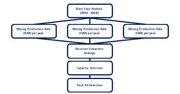
Figure 4. Base Case Definition Flowsheet
Source: Elaborated by the author, 2018
Later, and once the defined the production rate, there will be an analysis to find the correct Mineral Reserve extraction. This extraction strategy is made by selecting preliminary phases or nested pit sequence, where each of them must satisfy the processing plant feed capacity set at 10Mt per year during at least 2 periods. Also, based in the tonnage of each nested pit selected, the Project NPV should be maximized at an RF[3] equal to 1.
Finally, from the analyses previously made, the final pit shell generation is directed under some criteria such as Stripping Ratio or Life of Mine (LOM), even though the most important criteria is the NPV result. Hence, the Project can be executed in accordance with the Company parameters.
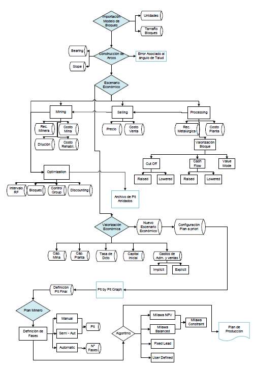
The above-mentioned is presented in a flowsheet at Figure 4 and this procedure will be completed over the use of the software Whittle® and its Milawa Algorithm®[4].
2.2 MINERAL RESERVE EXTRACTION STRATEGY
The strategy of extraction of reserves is dependable of the tonnage input to the processing plant (for this Project is 10Mt per year) and it seeks, at the same time, to obtain a high NPV value of the project by selecting at ends the right Project phases sequence.
2.2.1 PRELIMINARY PIT SEQUENCE ANALYSIS
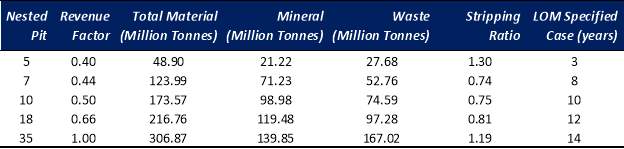
By using the software Whittle®, it can be determined the sequence that meets the feeding processing plant requirement, for at least two years. The result of this process is shown at Table 6 and it displays the sequences chosen for each production rate previously evaluated.
Table 6. Nested Pit Sequence Selected
Source: Elaborated by the author, 2018
2.3 MINING PRODUCTION RATE ANALYSIS
The goal of this section is deciding the best mining production rate for the Project, accommodated to feeding the processing plant which capacity cannot be changed. Table 7 shows the results’ summary and below more information on each analysis.
Table 7. Mining Production Rate and Selected Nested Pit Summary
Source: Elaborated by the author, 2018
2.3.1 MINE CAPACITY AT 26Mt PER YEAR
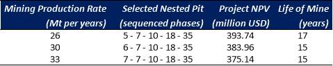
By restricting Whittle® at a mining production rate of 26Mt per year and utilizing the previous selected sequence at Chapter 2.2.1., the result for the Project NPV under these conditions is USD 393.74 million and a LOM of 17 years. The chart at Figure 5 shows the cumulated tonnage of material produced at 26Mt per year and the NPV of different cases (best, specific and worst-case scenario).
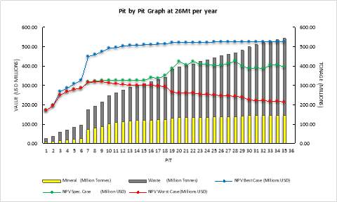
Figure 5. Pit by Pit Graph at 26Mt per year
Source: Elaborated by the author, 2018. Geovia, Whittle® (2014).
2.3.2 MINE CAPACITY AT 30Mt PER YEAR
By restricting Whittle® at a mining production rate of 30Mt per year and utilizing the previous selected sequence at Chapter 2.2.1., the result for the Project NPV under these conditions is USD 383.96 million and a LOM of 15 years. The chart at Figure 5 shows the cumulated tonnage of material produced at 30Mt per year and the NPV of different cases (best, specific and worst-case scenario).

Figure 6. Pit by Pit Graph at 30Mt per year
Source: Elaborated by the author, 2018. Geovia, Whittle® (2014).
2.3.3 MINE CAPACITY AT 33Mt PER YEAR
By restricting Whittle® at a mining production rate of 30Mt per year and utilizing the previous selected sequence at Chapter 2.2.1., the result for the Project NPV under these conditions is USD 375.14 million and a LOM of 15 years. The chart at Figure 7 shows the cumulated tonnage of material produced at 33Mt per year and the NPV of different cases (best, specific and worst-case scenario).
Figure 7. Pit by Pit Graph at 33Mt per year
Source: Elaborated by the author, 2018. Geovia, Whittle® (2014).
2.4 MINING PRODUCTION SCHEDULE
Despite the findings of the last section, where the highest NPV result is obtained at 26Mt per years, mining production schedule was developed to show the metal grades and ore, waste and total tonnes by year, throughout the life of the mine.
Based on the analysis made to determine the most appropriate production rate, the results of this analysis are presented at Figures 8 to 10 for each production rate; the fact that either at production rate of 26Mt per year and 30Mt per year are constant in mining production through the mine life, the input tonnage to processing plant is not.
In conclusion, the optimal mine capacity is recommended at 30Mt per year, which does not provide the highest Project NPV but has more coherence with the processing plant feeding, an important point to consider in development stage and Project 15-years LOM.
Regarding other mining production, at 26Mt per year is not feasible to satisfy the processing plant consistently during LOM although it presents the highest Project NPV. At 33Mt mining capacity, the Project NPV is the lowest and both mining and processing plant feeding rates are erratic.
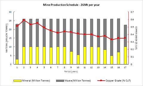
Figure 8. Mine Production Schedule at 26Mt per year Mining Production Rate
Source: Elaborated by the author, 2018. Geovia, Whittle® (2014).
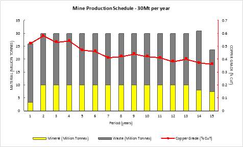
Figure 9. Mine Production Schedule at 30Mt per year Mining Production Rate
Source: Elaborated by the author, 2018. Geovia, Whittle® (2014).
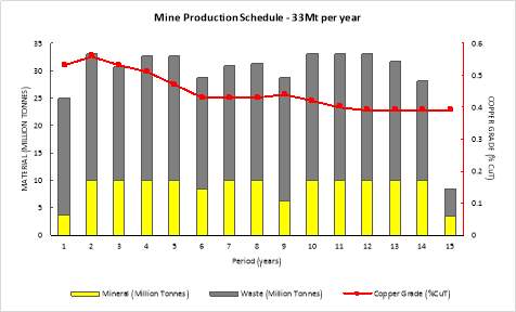
Figure 10. Mine Production Schedule at 33Mt per year Mining Production Rate
Source: Elaborated by the author, 2018. Geovia, Whittle® (2014).
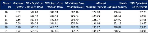
2.5 FINAL PIT SELECCION – BASE CASE
Founded on the information collected in preceding sections, it is required to define the final pit shell for the Project, which is obtainable from the 35 nested pits of the chart shown in Figure 6.
In building the most profitable Project for the Company, the analysis uses NPV as the main criteria for the final pit shell selection in this exercise (Appianing & Mireku-Gyimah, 2015). From the results (Table 8), pit 20 was selected based on Specific Case NPV value of USD 419.57 million.
Table 8. Final Pit Selection Options for Base Case
Source: Elaborated by the author, 2018.
Therefore, the final mining production plan for the selected final pit is shows at Figure 11.
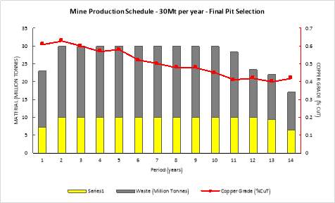
Figure 11. Mine Production Schedule at 30Mt per year – Final Pit Selected
Source: Elaborated by the author, 2018. Geovia, Whittle® (2014).
2.6 CHAPTER SUMMARY
Throughout the process of defining the Base Case to compare the angle influence in the Open Pit Project value against with, the Project was evaluated at different mining production rates.
In an initial stage, the mining production rate 26Mt per year provided the highest NPV. However, analyzing the production schedule, it was not able to meet the input processing plant feeding in a uniform manner.
The selected mining production rate was established at 30Mt per year, which has a maximum NPV of USD 419.57 million, over a LOM of 14 years. Total mineral production of 133.27 million tonnes with an average stripping ratio and copper grade of 1.95 and 0.51% CuT, respectively.
3.1 INTRODUCTION
Towards the analysis of the slope angle variation in an open pit project and set forth an option for the Company operation that well performs its Project, this project is considering the same applicable methodology shown in Figure 4 at Chapter 2.1.
Whereas the flowsheet presented in Chapter 2.1. enacts the analysis at different mining production rates, for the study proposed in this chapter the mining rate is set at 30Mt per year to compare apple-to-apple and avoid results distortions due the inclusion of more modifiable factors.
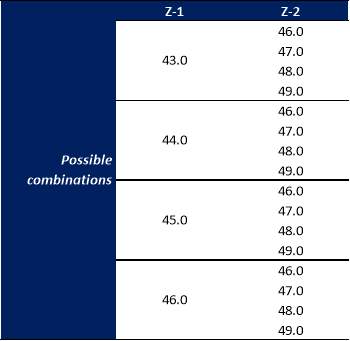
The geotechnical restrictions where presented in Table 4 and the possible combination created by the 4 angle options at Z-1 and Z-2 are shown in Table 9.
Table 9. Angle Combinations to Evaluation
Source: Elaborated by the author, 2018.
From these 16 iterations, the NPV value of each of them is shown in Figure 12.
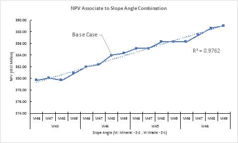
Figure 12. NPV Trend for Slope Angle Combinations
Source: Elaborated by the author, 2018.
As can be seen in the Figure above, there is a clear tendency towards an increase in the Project NPV value when the angles for mineralized and waste zones become steeper. This trend is explained due (1) the faster reach of mineralized zones and subsequently the prompt extraction of higher copper grades, and (2) the lower extraction and movement of waste material to strip the mineral (Contreras, 2005).
3.2 ALTERNATIVE ANALYSIS
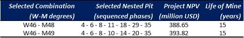
Such as occurred in the Base Case analysis, it is pertinent consider not only the option that sounds to be the best at first view. By that reason, the two highest combinations are being evaluated in this chapter (Alternative A: W46-M48 and Alternative B: W46-M49).
3.2.1 MINE PRODUCTION STRATEGY
From the selected alternatives for analysis, at a mining production rate of 30Mt per year and a processing plant feeding rate of 10Mt per year. The result for the Project NPV under these conditions is USD 388.65 million and a LOM of 14.92 years for Alternative A, meanwhile for Alternative B the Project NPV is USD 393.82 million and a LOM of 15.4 years. The pit by pit chart for each alternative are presented in Figures 13 and 14.
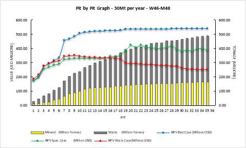
Figure 13. Pit by Pit Graph at 30Mt per year – Alternative A: W46-M48
Source: Elaborated by the author, 2018. Geovia, Whittle® (2014).
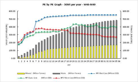
Figure 14. Pit by Pit Graph at 30Mt per year – Alternative A: W46-M49
Source: Elaborated by the author, 2018. Geovia, Whittle® (2014).
3.2.2 MINERAL RESERVE EXTRACTION STRATEGY
Contrary to what was settled in the Base Case regarding the extraction strategy and the selection of phases of the Base Case that remained stable (the variable parameter was mining production rate), the analysis for variation of slope angle let run every combination with its own sequence (Table 10).
Table 10. Selected Nested Pit for Alternatives
Source: Elaborated by the author, 2018
3.2.3 PRODUCTION SCHEDULE FOR SELECTED ALTERNATIVES
To select the appropriate alternative to compare with the Base Case is necessary to evaluate the mine production schedule.
At Figure 15 and Figure 16, are presented the mine production schedule for both alternatives.
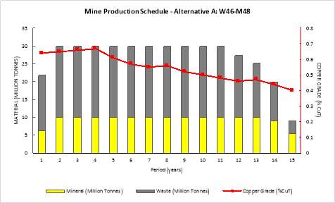
Figure 15. Mine Production Schedule – Alternative A: W46-M48
Source: Elaborated by the author, 2018. Geovia, Whittle® (2014).
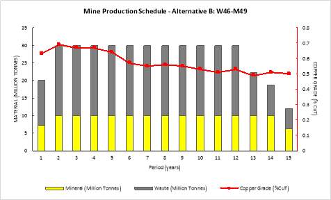
Figure 16. Mine Production Schedule – Alternative B: W46-M49
Source: Elaborated by the author, 2018. Geovia, Whittle® (2014).
These production plans were determined based on their selected sequenced phases to maximize the Project value and find the proper methodology to develop the reserve extraction of mineral.
From the above charts, both alternatives provide a smooth and constant processing plant feeding and a consistent mining production over LOM. However, Alternative B presents better results in terms of project final value, lower stripping ratio and higher copper grade reaching, hence Alternative B is selected and will be called Study Case hereinafter.
3.3 FINAL PIT SELECTION – STUDY CASE
Finally, and decided to compare the Base Case against Study Case supported in the parameters described above, the definition of the final pit shell for the Project Alternative is the next task of this analysis.
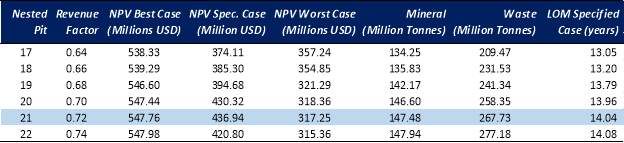
Based on the same criteria used in the Base Case, Project NPV, the final pit shell for Study Case is the nested pit 21 with the highest NPV value of USD 436.94 million as shown in Table 11. The final production schedule for Study Case is shown in Figure 17.
Table 11. Final Pit Selection Options for Study Case
Source: Elaborated by the author, 2018.
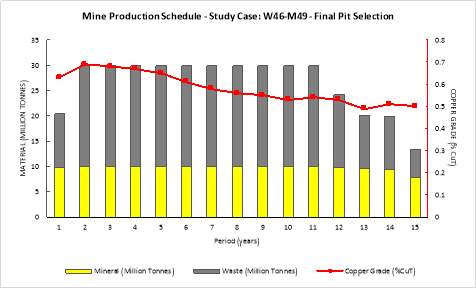
Figure 17. Mine Production Schedule – Study Case: W48-M49 – Final Pit Selected
Source: Elaborated by the author, 2018. Geovia, Whittle® (2014).
3.4 RESULT ANALYSIS
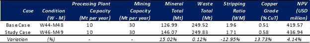
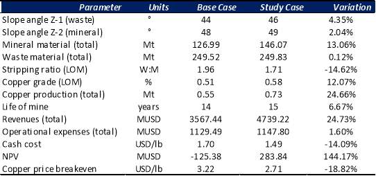
The results presented in Table 12, and compared the Study Case against the Base Case, show a clear increase in positive Project parameters and a decrease in the negative parameters.
A higher mineral recovery (+15.02%), bounded with higher copper grades (+13.73%), are traduced in an NPV increment of USD 17.37 million (+4.14%). Finally, the rise in the mineral recovered, and the decline in waste rock material, permits a lower stripping ratio of 1.71 (-12.95%) compared with 1.96 for the Base Case.
Table 12. Result Analysis Comparison Base Case (W44-M48) – Study Case (W46-M49)
Source: Elaborated by the author, 2018.
3.5 CHAPTER SUMMARY
In this chapter the different alternatives of slope angles provided by the Company, according to geotechnical restrictions, were evaluated. To achieve a comparison in line with the Base Case parameters, the mining production rate was set at 30Mt per year and only the slope angle was the measured variable.
As expected, the steeper the slope angle for the same project, the better the project NPV value, and therefore the considered alternatives for this study were the higher results (Alternative A: W46-M48 and Alternative B: W46-M49). These alternatives were optimized in production by looking for their best sequence phases and assessed on their production schedule.
The outcomes of this assessment indicate that Study Case (Alternative B) is which has better results in every parameter considered. Thus, Study Case was compared with the results of Base Case reached at Chapter 2, without exceed maximum slope angle for waste and mineralized zones.
Preliminarily, the application of Study Case offers a better economic return and operational design parameters than Base Case and is in accordance with the constraints allowing a safety mining operation as well.
4.1 INTRODUCTION
One important parameter to consider when changing the design in a mining project, both underground and open pit, is the equipment fleet selection and estimation (loading, hauling and support equipment.
It should be noted that the fleet estimation in this project does not include any operating design and the estimation is based on the mining production (mineral and waste production tonnage).
To calculate the mining fleet the information, the mine is scheduled to work 7 days per week, 365 days per year, but 15 days of lost time due to weather were allowed for in planning. Each day will consist of two 12-hour shifts. Four mining crews will rotate to cover the operation, with two-shifts on and two-shifts off (Fluor, 2017).
4.2 DRILLING EQUIPMENT
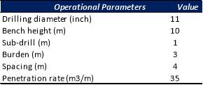
The main objective of this operation is to “create a physical space where the explosive is held, to then fracture the rock to be removed”. To carry out this operation, the parameters of the selected drill machine (model: PV-351) are shown in Table 13.
Table 13. Drilling Equipment Operational Parameters
Source: Elaborated by the author, 2018.
For simple calculations, each case will use one drilling equipment on mineral and another one on waste material. As a backup of operations, there will be considered a third one.
4.3 LOADING EQUIPMENT
The main objective of this process is “collecting the blasted material and load it adequately in trucks”. This is an important production process that involves large and high mechanized equipment in a continuous and slow operation.
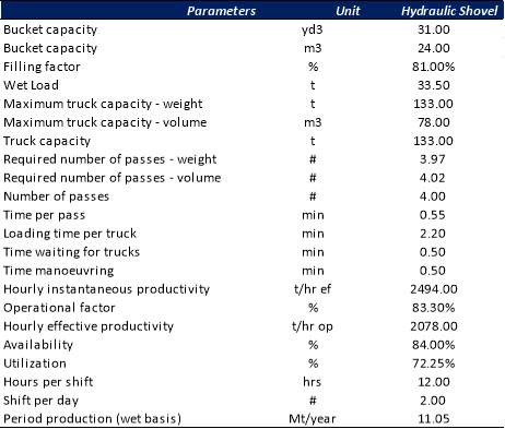
The performance of the loading units has been calculated based on the operational indices and detailed estimate of the time involved in loading. Table 14 shows the productivity calculation for loading equipment (model: 6060FS FO).
At Figure 18 is presented the distribution of shovels, both for Base Case and Study Case, for extraction of waste and mineralized material. The shovels distribution is regarding the amount of material and operationally the distribution for Study Case is more realistic to perform. However, an extra shovel will be required as a backup and included in investment calculation.
Table 14. Loading Productivity Estimate
Source: Elaborated by the author, 2018.
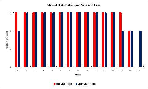
Figure 18. Shovels’ Distribution
Source: Elaborated by the author, 2018.
4.4 HAULING EQUIPMENT
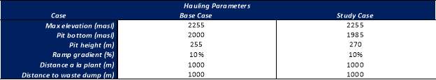
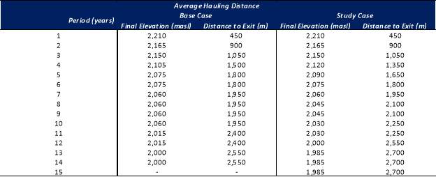
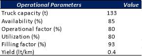
Once the material is collected, it must be transported to the respective destination (processing plant or waste dump facility [WDF]). At first instance, a distance profile must be calculated and using an in-house system parameter set (Table 15), the haulage distances were calculated on the same period basis as the production schedule for the pits, shown in Table 16.
Table 15. Hauling Parameters by Case
Source: Elaborated by the author, 2018.
At Table 17 are presented the operational parameters for hauling equipment (model: Cat 785D), and at Table 18 truck speeds were determined using typical values obtained from supplier information.
Table 16. Hauling Distance Summary by Case
Source: Elaborated by the author, 2018.
Table 17. Hauling Equipment Operational Parameters
Source: Elaborated by the author, 2018.
Source: Elaborated by the author, 2018.
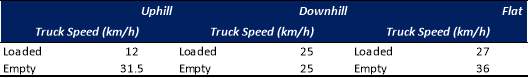
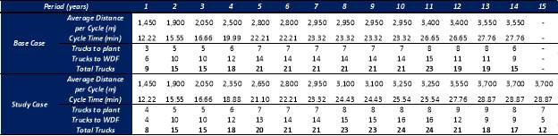
With this information (distances from Table 16, operational parameters from Table 17, and truck speeds from Table 18) it is possible to calculate the truck cycles and trucks requirements per period. A summary of this requirements is shown in Table 19.
Table 19. Cycle Time and Hauling Fleet Calculation Summary
Source: Elaborated by the author, 2018.
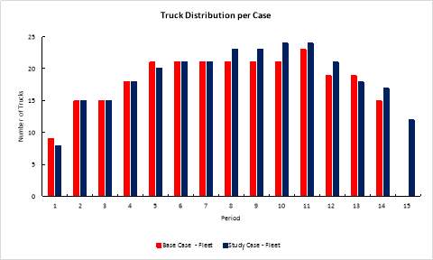
Figure 19. Trucks’ Distribution
Source: Elaborated by the author, 2018.
4.5 AUXILIARY AND SUPPORT EQUIPMENT
Major auxiliary equipment refers to the major mine equipment that is not directly responsible for production, but which is scheduled on a regular basis. Equipment operating requirements, operating hours, and personnel requirements were estimated for this equipment. The primary function of the auxiliary equipment is to support the major production units and provide safe and clean working areas (Contreras, 2005).
The primary duties that will be assigned to the auxiliary equipment are as follows:
- Mine development including access roads, drop cuts, temporary service ramps, safety berms
- Waste rock storage area control; this includes maintaining access to the dumping areas and maintaining the gravel surfaces
- Ore stockpile area control, including maintaining access to stockpile areas and maintaining operating surfaces
- Maintenance and clean-up in mine and waste storage areas, and water diversion channels around the WSFs and open pit
- Drilling for pre-split blasting
The estimated maximum quantities for the auxiliary and support equipment are detailed in Table 20. This equipment requirement is calculated as the same for both cases.
Table 20. Auxiliary and Support Equipment Requirement
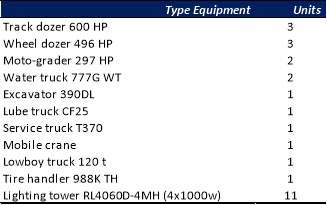
Source: Elaborated by the author, 2018.
4.6 CHAPTER SUMMARY
As a general footnote, all the manufacturer and model types are for orientation of equipment class only and not indicative of an equipment selection.
As production in both cases is quite similar between them, the equipment requirements do not present a great difference. Although, main variances appear at year 1 and at the second half of the both LOM projects. Altogether, Study Case is considered more suitable to put in practice and operation than Base Case due a less uneven requirement pattern.
5.1 INTRODUCTION
As a final stage for analyzing the Project feasibility and the proposed alternative, it is required to assess the study that has been carried out so far in the present Engineering Report in term of financial results.
To develop the economic evaluation and decide whether the Study Case can compete against the Base Case and its profitability, the following steps are been addressed:
- Revenues
- Mining Operating Expenses
- Cash Cost
- Investments
- Cash Flow
- Sensibility
5.2 REVENUES
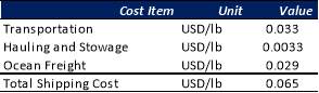
According to Company information, the final product of this Project is a copper cathode and it will be valued in accordance with the parameters mentioned in Table 5. Both options (Base Case and Study Case) are assessed under the same conditions and consider the transportation cost as follow (Table 21):
Table 21. Final Product Shipping Cost
Source: Elaborated by the author, 2018.
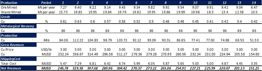
The calculation and results for Base Case and Study Case revenues are shown in Table 22 and 23, respectively. As well as, Table 24 shows a summary of this information.
Table 22. Net Revenues – Base Case
Source: Elaborated by the author, 2018.
Table 23. Net Revenues – Study Case
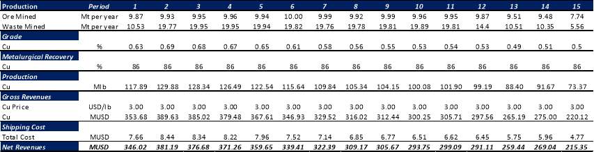
Source: Elaborated by the author, 2018.
Table 24. Net Revenue Comparison

Source: Elaborated by the author, 2018.
From the tables shown above, in both cases, the highest net revenue is reached in period 2, with MUSD 329.38 for Base Case and 381.19 for Study Case. This highest value is due for two reasons mainly, (1) the starting of mining production regime of 10 Mt per year and (2) the influence of high copper grade level at the beginning of operation (they are supposed to gradually reduce during the project life).
Overall, Study Case achieve better results than Base Case with a total net revenue value of MUSD 4,739.22 that represent close of MUSD 1,200 of difference. The Study Case average revenue is MUSD 61.13 higher than Base Case, considering the extra year of Study Case. The distribution of net revenues is also presented in Figure 20.
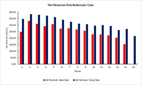
Figure 20. Net Revenue Distribution per Case
Source: Elaborated by the author, 2018.
5.3 MINING OPERATING EXPENSES
These costs have been subdivided into categories and/or unit operations, and their unitary cost has been benchmarked against similar-sized projects and length. The mine operating cost are summarized and totally calculated by period for each case in Table 26 and Table 27.
Besides, Figure 21 shows the distribution of operating expenses per period of each case and Table 25 displays the values of total expenses (in USD million and USD/t mined).
From Figure 21, and period by period, the Study Case possess a higher operating expense, apart from period 1, although in general, the operating expenses are lower according to Table 25.
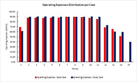
Figure 21. Operating Expenses Distribution per Case
Source: Elaborated by the author, 2018.
Table 25. Operating Expenses Comparison

Source: Elaborated by the author, 2018.
Table 26. Operating Expenses – Base Case
Source: Elaborated by the author, 2018.
Table 27. Operating Expenses – Study Case
Source: Elaborated by the author, 2018.
5.4 CASH COST
The Cash Cost concept involves all those costs incurred when carrying on the production, less revenues for sales of sub-products.
The Cash Cost value is considered a key factor when evaluating profitability and viability of a mining business because it measures the cost to produce one (1) tonne of ore in term of pounds/ounces.
In Figure 22, is shown the Cash Cost distribution of both analyzed cases and the similar pattern they follow, although Study Case has lower Cash Cost levels than Base Case. As well as, Table 28 shows the main figures of each case (Total Cash Cost in USD million and USD/lb)
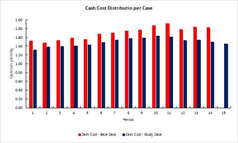
Figure 22. Cash Cost Distribution per Case
Source: Elaborated by the author, 2018.
Table 28. Cash Cost Comparison

Source: Elaborated by the author, 2018.
Table 29. Cash Cost – Base Case
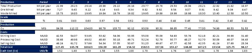
Source: Elaborated by the author, 2018.
Table 30. Cash Cost – Study Case
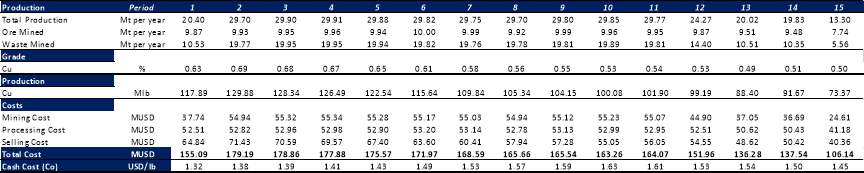
Source: Elaborated by the author, 2018.
5.5 INVESTMENTS
Under this item are covered all the expenses required to develop and give life to the project.
5.5.1 GENERAL AND ADMINISTRATIVE COSTS
Table 31 below provides details on all components of the general and administrative (G&A) costs. Due both cases are closely comparable in production, equipment and labor requirements, the G&A costs have been calculated as same.
Table 31. Detail of General and Administration Costs
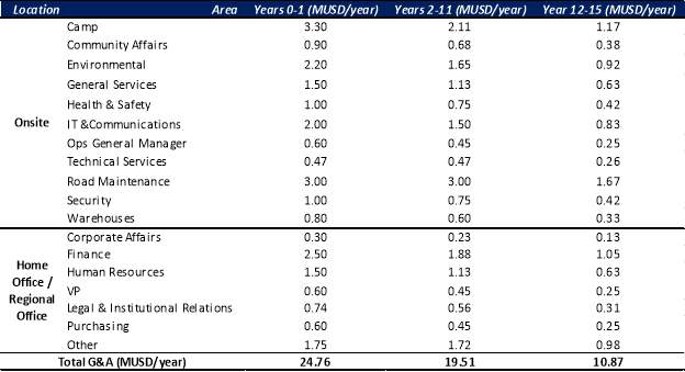
Source: Elaborated by the author, 2018.
5.5.2 EQUIPMENT COSTS
Capital cost estimates for mining equipment are developed so that these costs could be incorporated into the mining cost estimate to reflect the contractor’s capital recovery. This approach was suggested by the Company and applied since the contractor bids provided insufficient information on capital cost recovery. Typically, with mining contract, these costs are included in the operating costs.
The costs for the major equipment are based on vendor quotes obtained during Q3 2017. The costs for some minor equipment are based on quotations obtained during Q2 2016 and others from Mario’s employer database. Estimated freight costs for shipping the mine equipment to site and all costs to assemble the equipment are included in the estimates. Table 32 shows the details of the cost per unit.
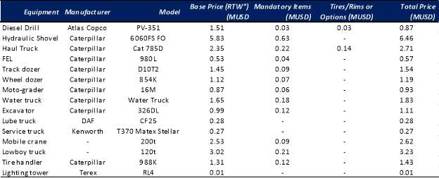
Note: Manufacturer and model types are for orientation of equipment class only and not indicative of an equipment selection
*RTW: Ready to Work
Source: Elaborated by the author, 2018.
The mining equipment initial capital for Base Case is USD 152.88 million and for Study Case is USD 154.55 million.
5.5.3 PROJECT CLOSURE COST
The project closure cost has been estimated based on the demolition/dismantling quantities provided by the Company from its own suppliers. The Company has consolidated the information in order to generate a complete project closure cost of US$30.2 million. The Company’s ancillary component of the closure cost represents US$8.8 million. This value includes personnel severance packages.
The total closure cost is US$39.1 million for both cases.
5.6 CASH FLOW
After revenues and discounted all the expenses incurred in production and give the Project life, the cash flows per period are determined as shown in the next figures and tables.
The comparison of Project cash flows is summarised in Figure 23, and individual cash flows are presented for both cases in Figures 24 and 25, for Base Case and Study Case respectively. The initial flow shows the Capex and production stream in the project’s later years.
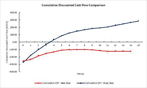
Figure 23. Cumulative Discounted Cash Flow Comparison
Source: Elaborated by the author, 2018.
As shown in Figure 23 above, a quick payback of close to 3 years and the positive NPV of the Study Case results, are the main strengths of the project. In both cases, the initial investment reaches similar levels, even though the incomes received in the Base Case are not enough to cover the expenses and provide a positive NPV result for this Project (Figure 24 and Figure 25).
The cash flow information per period is presented in Tables 34 and 35, for Base Case and Study Case separately.
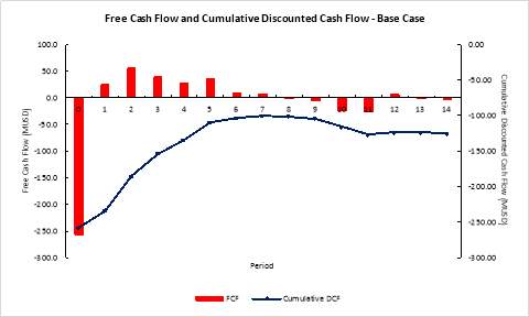
Figure 24. FCF per Period and Cumulative DCF – Base Case
Source: Elaborated by the author, 2018.
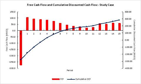
Figure 25. FCF per Period and Cumulative DCF – Study Case
Source: Elaborated by the author, 2018.
Table 33. Cash Flow per Period – Base Case
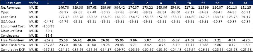
Source: Elaborated by the author, 2018.
Table 34. Cash Flow per Period – Study Case
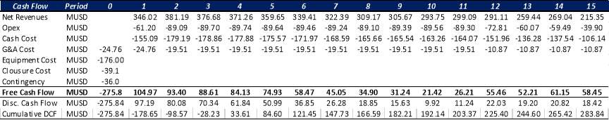
Source: Elaborated by the author, 2018.
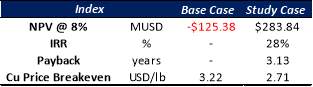
Table 35. Comparison of Economic Valuation Results
Source: Elaborated by the author, 2018.
In terms of project return and business impact, Table 33 summaries the information of the cash flow streams. For Base Case, the results are not positive under the evaluated parameters. However, the Study Case presents positive results, the NPV of the Project is MUSD 238.84 million, with an IRR of 28% and Copper price breakeven of 2.71 USD/lb (these figures do not consider taxation).
5.7 SENSITIVITY ANALYSIS
Scenario analysis was performed to estimate a range of potential return for the project by varying key assumptions of the financial model. These analyses are not meant to represent all possible ranges, but rather the Project’s estimate for reasonable downside and upside scenarios.
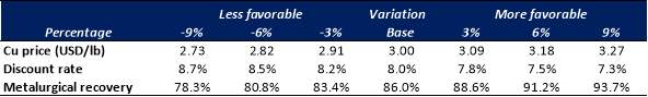
The main assumptions for the project value are Copper prices, followed by the discount rate, and metallurgical recovery. Table 36 shows the variation of the value for these parameters for sensitivity analysis.
Table 36. Parameter Variation for Sensitivity Analysis
Source: Elaborated by the author, 2018.
In addition, Table 37 and Table 38 show the NPV value of each case after applying the modified parameters, including the combination of all these parameters. Also, the Figures 26 and 27 show the graphical representation of these modified parameters.
Analyzing the Base Case is found that only a favorable increase closely to 6% in Copper price and metallurgical recovery allows a positive NPV result. If all these parameters move in a favorable direction, a positive NPV is reached at a variation close to 3% (Table 37 and Figure 26).
Table 37. Sensitivity Analysis Results – Base Case
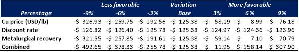
Source: Elaborated by the author, 2018.
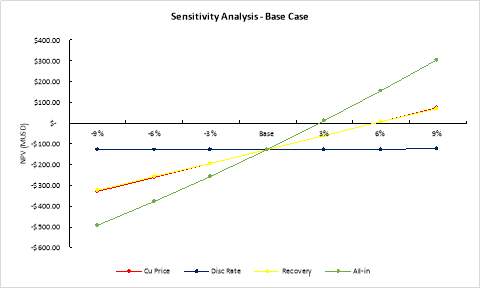
Figure 26. Sensitivity Analysis – Base Case
Source: Elaborated by the author, 2018.
Study Case remains positive NPV results under the variation of the parameters used in the sensitivity analysis. Only a modification of all these parameters in a negative direction, over 5%, will make the NPV result be negative (Table 38 and Figure 27).
Table 38. Sensitivity Analysis Results – Study Case
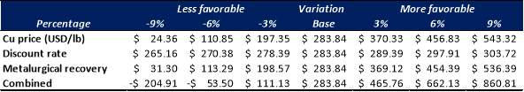
Source: Elaborated by the author, 2018.
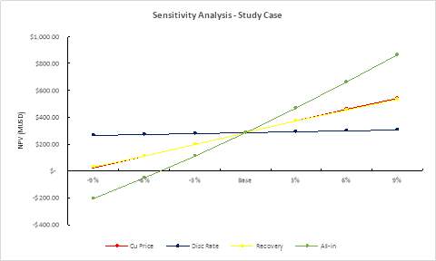
Figure 27. Sensitivity Analysis – Study Case
Source: Elaborated by the author, 2018.
5.8 BASE CASE AND STUDY CASE COMPARISON SUMMARY
Table 39. Comparison Summary Base/Study Case
Source: Elaborated by the author, 2018.
5.9 CHAPTER SUMMARY
In this chapter the two options achieved to develop the Project were analyzed from a financial viewpoint, seeking for generation of revenues and comparing them with the expected expenses to be incurred to reach the production. By doing this study and separately analyzing each project is was possible to find the best option for the Project and Company in terms of profitability.
In general, the Study Case showed better economic results than Base Case, driven by some variables that made predictable this outcome. These variables and its repercussion are the following:
- Stripping Ratio: Although the value for waste material extractable in both cases is similar, the amount of mineral is higher in Study Case than Base Case, giving a better stripping ratio and making the Project more profitable.
- Copper Grade: Study Case no only has more tonnes of mineral material, but also has better copper grades on average than Base Case, with the highest values at the beginning of the operation. Relating this aspect with the time value of money (TVM), the consequence of extracting more material with more metal contained has more influence into the Project NPV.
- Life of Mine: Although Base Case counts with better total results for expenses (lower expenses), the prorated value in the life of mine operation years does not indicate the same tendency. As Study Case is longer than Base Case the average expenses per year are lower.
These conditions and the performed evaluation delivered as a result the best option for the Project is the execution of the Study Case and therefore apply the slope angle variation offered.
From the sensitivity analysis, it can be seen the more impressionable variables are either Copper Price and Metallurgical Recovery, displaying a very related upshot for NPV value.
Fortunately for Study Case performance, the Metallurgical Recovery is impractical to suffer variation unless the processing plan face problem in operation, and so far, this year the average Copper Price has been 3.01 USD/lb and as the October 2018 average Copper Price is 2.79 USD/lb.
Sensitivity analysis shows a strong basis for Study Case in the long run and over Project life of mine.
A final section of this Engineering Project, conclusion and recommendations that were found during this study, are presented as follow:
6.1 CONCLUSIONS
Undoubtedly and with the presented results along this project, this study shows the sensitivity of the Project for slope angle approximations and an increase in its value, and therefore a higher benefit for the Company. Some of the outcomes that enable this result are the amount of mineralized material extracted in the Project life of mine, which reduces the average stripping ratio and operating expenses, and the extension of Project’s life, making distributing in a better manner the resources (equipment) and allows a reduction in the average cash and investment costs, due an extended apportionment of costs.
A step-by-step tour through this Engineering Project, allows as to find the next conclusion:
- By selecting a suitable mining production rate for the Project, 30Mt per year (around 85,000 tonnes/day) achieve the most appropriate result for Base Case. The selection of this mining production rate obeys not only on choosing the highest NPV for the project, but also a constant processing plant feeding. A 30Mt mining rate allows supplying 10Mt per year of required mineral to the processing plant, avoiding uneven production inputs during operation.
6.2 RECOMENDATIONS
A more thorough
Appianing, E. J., & Mireku-Gyimah, D. (2015). Open Pit Optimisation and Design: A Stepwise Approach. Nkroful, Nzema East District: Ghana Mining Journal.
Bereta, F., & Marinho, A. (2014). The Impacts of Slope Angle Approximations on Pit Optimization. Research Gate, 2-15.
Castillo, L. (2009). Modelos de Optimizacion para la Planificacion Minera a Cielo Abierto. Santiago: Universidad de Chile, Facultad de Ciencias Fisicas y Matematicas, Departamento de Ingenieria de Minas.
Company. (2015). Block Model. Project Block Model. Santiago, Chile.
Contreras, E. (2005). Mineria Cielo Abierto, Curso Diseno Rajo Abierto. Technical Refreshment, Gerencia Mina Division Andina Codelco Chile. Santiago.
Cunningham, C. e. (2008). Quantitative mineral resource assessment of copper, molybdenum, gold, and silver in undiscovered porphyry copper deposits in the Andes Mountains of South America. U.S. Geological Survey. Retrieved Sep 25, 2018, from https://pubs.usgs.gov/of/2008/1253/
Fluor. (2017). “Project” Pre-Feasibility Study (PFS), “Company”. Santiago: N/A.
Gemcom Software International Inc. (2008). Gemcom Whittle. N/A: Gemcom.
Gemcom Software International Inc. (2008). Milawa Algorithm(R) Module. N/A: Gemcom.
Gutierrez, L. (2016). Open Pit Optimization. Santiago: Universidad de Santiago de Chile.
Martinez, M., Miranda, R., Morales, M., Venegas, N., & Zuniga, M. (2016). Estudio de Pre-Factibilidad de un Proyecto Minero de Tipo Cielo Abierto. Final Project – Prepared for Sebastian Vera, Universidad de Santiago de Chile, Departamento de Ingenieria en Minas, Santiago.
Muncher, B. (2016). Economic Assessment and Mine Production Optimization of an Open-Pit Gold Mine Operation in Peru, Based on the Iterative Cut-Off Grade Analysis Approach. Philadelphia: The Pennsylvania State University, The Graduate School, College of Engineering.
Read, J., & Stacey, P. (2009). Guidelines for Open Pit Slope Design. CSIRO Publishing.
SRK Consulting. (2015). Scoping Study “Project” – Preliminary Geotechnical Design. Memo prepared for “Company”. Santiago: N/A.
SRK Consulting. (2015). Scoping Study “Project” – Stability of Inter-ramp and Overall Slopes. Memo prepared for “Company”. Santiago: N/A.
APPENDIX A. Whittle® and Milawa Algorithm®
Whittle®: Strategic Mine Planning Tools for Enginners, Geologists and Mine Planners (Gemcom Software International Inc., 2008)
When mining companies seek to maximise NPV, balance schedules, and to optimise blends and stockpiles, they use Gemcom Whittle. Whittle delivers trusted results and is used in scoping, feasibility, life-of-mine scheduling, and in the ongoing re-evaluation of mine plans throughout the production phase.
Because pit optimization alone is not enough to unlock the full economic potential of your operation, Whittle provides mine optimization, which enables significant increases in project value over and above pit optimization.
Benefits:
Exploration
- Understand the potential value of the deposit.
- Target areas for future drilling.
Scoping
- Establish the economic viability of the deposit and options for capital investment and development strategies.
- Examine sensitivities and assign resources accordingly for future studies.
Pre-feasibility, Feasibility
- Identify preferred development strategy, capital investment, expected NPV and optimal extraction sequence.
- Calculate sensitivities to develop risk reduction strategy.
- Ascertain final reserve statement for the deposit.
Bankable Feasibility
- Study expected return on investment.
- Analyze sensitivities and investment risk.
- Consider multiple scenarios for reducing risk.
Production
- Determine strategic direction for the mine; cut-off grade and optimized cut-off grade; mining areas and extraction sequence per period; and development strategies for new mines and push backs.
- Re-evaluate mine plans in response to changing conditions.
- Calculation of annual reserve statement.
Whittle Modules:
Multi-Element – This extends the capabilities of Whittle to allow up to ten elements to be defined in the model. Individual elements and reported separately and the grades and quantities of each element are available for use in user-defined expressions, graphs and reports.
Mining Width – This adjusts pushbacks to allow for mining width constraints. The speed and repeatability of the process means that users can experiment with different mining widths to see what impact they have.
Milawa Algorithm – This module schedules pushbacks in order to maximise NPV or to balance the mining rate. It responds to all production constraints, price and cost models within Whittle and also provides additional controls over the schedule.
Multi Analysis – This module significantly extends the capabilities of Whittle by allowing multiple imported models per project, and branching of the analysis trees thereafter.
Advanced Analysis – This module allows Four-X Analyser to perform very complex analysis. This is extremely useful to designers who are interested in extensively testing sensitivities and performing risk analysis.
Stockpile and Cut-off Optimisation – This module provides comprehensive grade-stockpile and cut off optimisation with the objective of maximizing NPV. The model re-schedules the mining sequence, taking in to account all the constraints and setting in Whittle and optimising the stockpile utilisation and cut off strategy.
Buffer Stockpiles – Use the Buffer stockpiles module to store material for future periods to avoid future stripping hurdles or to balance mining and processing rates.
Blending – This module optimises the blend, and the stockpile usage and when combined with Whittle Milawa Algorithm®, also optimizes the scheduling of the mine. All this is driven by the overall objective of maximising the NPV of the whole operation.
Milawa Algorithm® Module: Schedule to Maximise NPV (Gemcom Software International Inc., 2008)
The Milawa Algorithm ® adds a new dimension to life-of-mine scheduling. It optimises the schedule, taking into account all your production and economic constraints, while seeking to maximise the utilization of available mining and processing capacity.
The Milawa Algorithm® is a proprietary algorithm which schedules phases in order to maximise NPV. It responds to all production constraints, price and cost models within Four-X Analyser and also provides additional controls over the schedule.
How does it work? The Milawa Algorithm® consists of three parts:
• The first part takes a set of variables and generates a feasible schedule from them. A full set of the variables describes the life of mine schedule. The number of variables required depends on the number of benches in the ultimate pit, pushbacks, and time periods in the life of the mine. The possible values for these variables are constrained by what is technically feasible in terms of the pit shell precedence rules and any constraints imposed by the user (mining, processing, selling constraints, maximum and minimum lead, maximum vertical advance per period).
• The second part is an evaluation routine, which calculates the NPV for an individual schedule.
• The third part searches the domain of feasible schedules for the one, which has the highest NPV. This routine also has logic built in to decide when to stop searching.
Milawa does not generate and evaluate all feasible schedules as the number of feasible schedules can be extremely large. Rather it strategically samples the feasible domain and gradually focuses the search (without necessarily narrowing it) until it converges on its solution. The number of evaluations required to converge on a solution varies, but 5000 is typical, and this usually takes less than a minute.
The following image shows the detailed in the Whittle process:
[1] USGS: U.S. Geological Survey in the report “Do We Take Minerals for Granted?”
[2] Due confidentiality agreements, the Company’s and Project’s name, as well as every other reference to the real information of them, such as Project location, will be named as generic (i.e. Company, Project)
[3] RF: Revenue Factor, copper price weighted factor. The Project is evaluated a long-term copper price of USD 3.00/lb.
[4] Whittle® and Milawa Algorithm® information at Appendix A.
Cite This Work
To export a reference to this article please select a referencing stye below:
Related Services
View all


Related Content
All TagsContent relating to: "Environmental Studies"
Environmental studies is a broad field of study that combines scientific principles, economics, humanities and social science in the study of human interactions with the environment with the aim of addressing complex environmental issues.
Related Articles

DMCA / Removal Request
If you are the original writer of this dissertation and no longer wish to have your work published on the UKDiss.com website then please: