Biaxial Driving of Piezoelectric Actuators for Ultrasound
Info: 13050 words (52 pages) Dissertation
Published: 9th Dec 2019
Tagged: ElectronicsMedical Technology
Biaxial Driving of Piezoelectric Actuators for Ultrasound
ABSTRACT
Over the years, piezoelectric materials have been used in a wide variety of application on the health care field in the form of ablation and therapeutic treatments, medical imaging and lithotripsy, just to mention some of them. A more efficient operation of ultrasound transducers translates into less power consumption to obtain the desired effect. Commonly used ferroelectric actuators are driven by applying the electric field along the poling axis in order to maximize their mechanical response. The biaxial driving technique enhances the mechanical response of a piezoelectric actuator by dephasing two orthogonal electrical fields to the propagation and lateral electrodes. In this approach, several parameters are going to be tested to improve the acoustic efficiency response of transducers biaxially driven. These results will lead to evaluate the application of the biaxial driven technique on ultrasound imaging transducers.
Table of contents
2.2 Ultrasound in medical applications
2.2.2.2 High intensity focused ultrasound
2.3 Acoustic propagation and acoustic wave
2.4 Characteristics of ultrasound
2.4.1 Frequency – Period – Wavelength
2.4.4 Attenuation and Absorption
2.4.5 Specular Reflection and refraction
2.8 Single element ultrasound transducer
2.8.2 Piezocomposite transducers
2.8.3 Capacitive micromachined ultrasound transducers (CMUT)
2.9.1 Piezoelectric charge constant
2.9.3 Electromechanical coupling factor
2.9.4 Piezoelectric voltage constant
2.9.5 Dielectric dissipation factor
2.10 Biaxial driving technique
3.- RESEARCH OBJECTIVES AND APPROACH
4.1 Biaxial transducer manufacturing process
4.2 Biaxial transducer efficiency characterization
4.3 Frequency sweep experiments
4.4 Power variation experiments
5.1 Power efficiency vs. Electrical power
1.- Introduction
Piezoelectric materials are used in a wide variety of medical application such as medical imaging, ablation and lithotripsy therapy treatments, to mention some of them. Piezoelectric materials for medical ultrasound transducers require high thickness mode electromechanical coupling coefficient (kt), high dielectric constant (KT3), low acoustic impedance, low dielectric loss and high mechanical strength [1]. Some piezoelectric materials can improve its dielectric, piezoelectric and ferroelectric properties by using a doping material such as Gd, Al or Ce [2-4]. Also, the use of different geometries and arrays on ultrasound transducers can enhance the electrical and acoustic performance [5]. The efficiency of a piezoelectric actuator is determined by the amount of electrical power converted into acoustic power. Higher efficiency translates into less electrical power needed to achieve the desired acoustic power, leading to a reduced heating on the transducer and less power consumption by the system.
A method to increase this efficiency is using the biaxial driving technique [6]. The biaxial driving technique is based on the polarization rotation achieved by dephasing two orthogonal sinusoidal electrical fields along the x (lateral) and z (propagation) axis of a piezoelectric actuator to reduce the coercivity produced by the ferroelectric switching resulting in an enhanced mechanical response [6-9]. Results on [6] showed that the output acoustic power from a biaxial transducer depends on the phase difference of the applied electrical fields, which is different at every transducer and needs to be characterized for all of them.
The goal of this research work is to demonstrate the feasibility of driving piezoelectric actuators with the biaxial driving technique. For this purpose, twenty biaxial transducers were fabricated and characterized. Transducer were cut to have resonant frequencies as similar as possible in both orthogonal directions. The acoustic effective power of the biaxial transducers was measured with a radiation force method and compared with transducers driven by using a single electrical field.
2.- Background
2.1 Ultrasound
Sound is a phenomena that involucres the propagation of a mechanical wave through a medium. It can be propagated thought liquid, solid or gaseous elastics media [10]. Ultrasound refers to an acoustic wave whose frequency is above the range of audible frequencies for human beings, which is approximately 20 Hz to 20 kHz. In acoustics, waves are classified as follow:
- Longitudinal waves, which consists in alternated compressions and rarefactions along the propagation direction in which the particles transmit the wave when moving back and forth from their equilibrium position parallel to the movement axis of the wave [11]. The propagation speed is determined primarily by the properties of the medium. Will be changes in the particle displacement, velocity, density, pressure and temperature associated with the wave propagation. [12].
- Transversal waves, which consist in perpendicular vibrations along the direction of propagation. In contrast to the changes in particle volume that occur for longitudinal waves, no density change occurs for transverse waves. Transverse waves cannot be propagated in liquids [12].
- Rayleigh waves consist of surface acoustic waves and are the result of the combination of the longitudinal and transverse waves. Each molecule runs an ellipse as the wave passes through it. This phenomena is produced when a longitudinal wave is tried to be generated on a surface which is in contact with air [10].
2.2 Ultrasound in medical applications
Ultrasound in the medical field can be found in a wide range of applications which can be divided into two major categories: Diagnostic and therapeutic. The frequency used on any specific application is based on the considerations of sound absorption, penetration and, in the case of diagnostic, resolution [13].
2.2.1 Diagnostic ultrasound
The diagnostic medical sonography (sometimes called ultrasonography), is an ultrasound-based image technique used to visualize subcutaneous body structures as tendons, muscles, joints and internal organs [14]. Sonographers are typically used with a hand-held probe (transducer) which is placed and moved over the patient body. Water based gels are used as a coupling between the probe and the body. Usually, the frequency range for ultrasonography lies between 2 and 18 MHz and is very effective for imaging soft tissues [14]. There are four different modes for ultrasound imaging:
- The A-mode (amplitude modulation) is the most basic of the four. It is primary used to make internal distance measurements.
- In the B-mode, an array of transducers scans a plane through the body by moving the probe over the surface. The received echoes can be reconstructed to produce a 2-D image.
- The M-mode (motion) employs brightness modulation and is used to observe the movement of anatomic structures [13].
- The doppler mode, as its name states, uses the doppler effect to measure and visualize the blood flow. It can also be used to detect fetal heart rate [13].
Because of the low cost of this technology and being a non-invasive technique with a quick scan, benefits of portability, real time examination, and that do not produces radiation, it is well accepted by patients [15].
2.2.2 Therapeutic ultrasound
The versatility of ultrasound in medical therapies relies in the interaction with the cells and tissues. Ultrasound can induce effects not only though heating, but by the generation of ultrasonic cavitation (growth and collapse or motion of bubbles), gas body activation or mechanical stress [16]. The type of effects produced by the interaction of the tissues with ultrasound waves depends on several parameters, but the most important are the frequency, duty cycle and amplitude of the ultrasound wave [17]. Therapeutic applications can be divided in thermal applications, including physiotherapy and high intensity focused ultrasound, and non-thermal applications, like lithotripsy.
2.2.2.1 Physiotherapy
Commonly known as therapeutic ultrasound. Its objective is to warm tendons, muscles and other tissues by improving blood circulation to accelerate healing. It uses a hand-held probe which is placed on the surface of the tissue by using a water-based gel. The probe is moved on circles around the surface of the treating zone by a technician. The level of benefits are uncertain and the risk of getting burned is low if it is properly applied [16].
2.2.2.2 High intensity focused ultrasound
The high intensity focused ultrasound (HIFU), is a thermal ablation technique generally used for oncological treatments. A focused transducer generates an ultrasonic beam which is concentrated on a focal zone. The temperature on the focal zone raises until a lesion of a few mm in diameter is produced on the zone without damaging the surrounded tissues. This method is approved by the FDA to treat uterine fibroids [18], essential tremors [19], pain palliation of bone metastatic cancer [20] and to produce ablation of prostatic tissue [21].
2.2.2.3 Lithotripsy
Known as shock wave lithotripsy, this technique uses ultrasound waves to destroy targeted kidney or bladder stones at a slow rate. Its effects are based on two fundamental mechanisms, shock wave-related effects and cavitation phenomenon [22].
2.3 Acoustic propagation and acoustic wave
The physical nature of the medium can be modeled as stationary, with a spatially varying density
[35]. Typical piezoelectric polymers have a crystalline region with a dipole moment randomly oriented without any mechanical or electrical poling process with a net dipole moment equal to zero in this condition. This type of structure is called the
α
-phase PVDF film and has not a piezoelectric response [36]. By applying a mechanical stretching and electrical poling under a high electric field, crystalline regions inside the bulk PVDF film will align in the electric field direction. This type of structure is called the
β
-phase PVDF film and exhibits piezoelectricity [36]. One of its most important applications is broadband hydrophones [35].
2.8.2 Piezocomposite transducers
Conventional piezoelectric ceramics such as PZT, lead metaniobate and modified lead titanates are useful for making ultrasonic transducers used in medical imaging because of their high electromechanical coupling coefficients. Their principal limitation lies in their high acoustic impedance which makes coupling to tissue difficult. Piezoelectric polymers, such as polyvinylidene difluoride (PVDF), present a different set of material properties. Their low acoustic impedance simplifies efficient coupling, but their low electromechanical coupling, low dielectric constant and high dielectric losses present additional limitations when integrating these materials into medical imaging transducers [37]. Simply stated, a piezocomposite is a combination of a piezoelectric ceramic and a non-piezoelectric polymer to form a new piezoelectric material with the properties enhanced. In general, however, the term piezocomposite applies to any piezoelectric resulting from combining any piezoelectric polymer or ceramic with other non-piezoelectric material [38]. The advantage of such arrangement is that it combines the superior piezoelectric properties of the chosen ceramic with the lower acoustic impedance of the polymer [12]. This type of transducers are fabricated with common piezoelectric materials, but not in one piece. The material is selected and filled with a vibration absorbent material to isolate every cut on the piezoelectric [10]. In a two-phase system, e.g., ceramic and polymer, there are ten possible connectivities, of which only a few are of practical interest for transducer fabrication [12].
2.8.3 Capacitive micromachined ultrasound transducers (CMUT)
CMUTS are micromachined transducers formed from numerous unit cells electrically connected in parallel, with each cell consisting of a metalized membrane suspended above a heavily doped silicon substrate (top and bottom electrodes, respectively) [39]. Fig. 6 represents the CMUTs unit cell.
Fig. 6.Schematic cross section of a CMUT unit cell [39].
During operation, a dc voltage is applied between both electrodes. This dc bias voltage causes the membrane to deflect downward to a static operating point which determines the sensitivity, frequency response and total acoustic pressure [40]. If an alternating voltage is superimposed on the bias voltage the modulation of the electrostatic force results in the vibration of the membrane with subsequent generation of ultrasonography at the same frequency of the modulation [41]. Conversely, if the biased membrane is subjected to ultrasound waves, a current output is generated as a result of a capacitance changes due to membrane vibrations.
The advances in microfabrication technology have made possible to build capacitive ultrasound transducers competing with piezoelectric transducers. CMUTs offers advantages of improved bandwidth, ease of fabrication of large arrays with individual electrical connections, and integration with electronics [39]. CMUTs are fabricated using silicon micromachining methods with submicrometer accuracy and uniformity, which allow fabrication flexibility. Since silicon micromachining determines the shapes, sizes and spacing between neighboring elements, flexible shapes and multiple elements with transducer spacing as small as 3 µm can be fabricated [40].
Besides medical and underwater imaging, CMUTS have some potential applications that include air-coupled non-destructive evaluation, ultrasonic flow meters for narrow pipelines, microphones with RF detection and smart microfluidic channels [41].
2.9 Material parameters
2.9.1 Piezoelectric charge constant
The piezoelectric charge constant dxy represents, for the direct piezoelectric effect, the polarization generated per mechanical stress (T) applied to a piezoelectric material and for the inverse piezoelectric effect, the mechanical strain (S) experienced by a piezoelectric material per unit of electric field applied. The subscript x represents the direction of polarization generated in the material or the direction of the applied strenght when the electrical field, E, is equal to zero. The subscript y indicates the direction of the applied stress or induced strain, respectively [32].
2.9.2 Permittivity
The permittivity or dielectric constant
εxyz
for a piezoelectric material is the dielectric displacement per unit electric field. Z is equal to T to represent the permittivity at constant stress, and equal to S to indicate the permittivity at constant strain. The subscripts x and y represents the direction of the dielectric displacement and the direction of the electrical field, respectively. [32].
2.9.3 Electromechanical coupling factor
The electromechanical coupling factor
kxy
is an indicator of the effectiveness with which a piezoelectric material converts electrical energy into mechanical energy, or convert mechanical energy into electrical energy (direct and indirect piezoelectric effect, respectively). The subscripts x and y denotes the direction along which the electrodes are applied and the direction along which the mechanical energy is applied or developed [32].
2.9.4 Piezoelectric voltage constant
The piezoelectric voltage constant
gxy
is the electric field generated by a piezoelectric material per unit of mechanical stress applied or the mechanical strain experienced by the material per unit of electric displacement applied. The subscripts x and y indicates the direction of the electrical field generated in the material and direction of the applied stress or induced strain [32].
2.9.5 Dielectric dissipation factor
The dielectric dissipation factor,
tanδ
, express the parasitic loss that results by subjecting a material to alternating electrical fields. It is a measure of the electrical loss of the materials. When an electrical field, E, is applied to an ideal dielectric material, the resultant charging current find itself out phase by 90° with the applied electrical field. However, in a real ferroelectric material, the current also has a loss component in phase with th applied E and the net resultant current makes an angle
δ
with the ideal charging current. This loss current is a result of the dissipation of energy heat. This loss can be interpreted using the parameter
tanδ
which is the ratio of loss current I’’ and charging current I’ [32].
| tanδ=I”I’ | (31) |
Typical values for some of the above parameters, for some important materials, are listed on Table 1.
TABLE 1
Piezoelectric Materials Properties [23]
| Quartz | PZT-4 | PZT-5A | Lead metaniobate | PVDF | |
| Dielectric constant | 5.0 | 1300 | 1700 | 22.5 | 8 |
| Coupling factor:
k33 |
01 | 0.7 | 0.7 | 0.38 | 0.19 |
| Piezoelectric constant:
d33 |
2 | 290 | 370 | 85 | 17.5 |
| Dissipation factor:
tanδ |
10-4 | 0.004 | 0.02 | 0.01 | – |
| Acoustic impedance:
Z106 Rayl |
15.2 | 34.5 | 33.7 | 20 | 3.4 |
2.10 Biaxial driving technique
Commonly used ferroelectric actuators are driven by applying the electric field along a poling axis to maximize their mechanical response [42]. Low coercivity and low hysteresis loss are desired properties for ferroelectric materials used in high power and high frequency applications [9].
In addition to the reorientation of polar domains by an applied electrical field, a polarization rotation was proposed [43] to describe a piezoelectric enhanced response in PZN-PT and PMN-PT single crystals, where a non-aligned field alternates the material strain vectors between tetragonal and rhombohedral configurations [6]. During the structural transformation associated with the polarization rotation, the polarization vector P does not disappear, it just changes its direction and maintains a magnitude similar to the spontaneous polarization P0 (Fig. 7) [6]. The energy surface for single-domain ferroelectric PbTiO3 calculated from first principles [9] is shown in Fig. 7. The lowest and highest energy corresponds to the tetragonal and cubic structures, respectively.
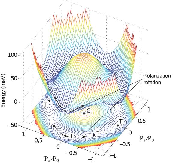
Fig. 7. Energy surface for polarization inversion in the (0 1 0) plane of PbTiO3. C, T and O refers to cubic, tetragonal and orthogonal structures, respectively. The narrows indicate evolution of polarization in a rotational manner [6].
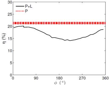
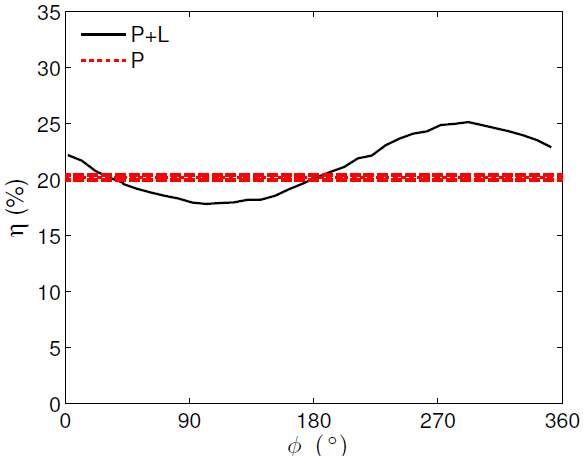
By doing experimentation with ferroelectric switching in PbTiO3, the results on [9] suggest that is possible to reduce coercivity (threshold at which the polarization switching occurs) and consequently the energy dissipation during operation of ferroelectric transducers by employing a two-dimensional excitation with modulation on the applied electrical fields. An experimental validation using PZT transducers was presented on [6] by comparing the acoustic efficiency of PZT transducers excited with a single electrical field vs. PZT transducers excited with two orthogonal electrical fields (biaxial driving technique). Results on [6] showed that the output acoustic power from a biaxial transducer depends on the phase difference of the applied electrical fields (Fig. 8), which is different at every transducer and needs to be characterized for all of them.
The biaxial driving technique is based on the polarization rotation achieved by dephasing two orthogonal sinusoidal electrical fields along the x (lateral) and z (propagation) axis of a piezoelectric actuator to reduce the coercivity produced by the ferroelectric switching resulting in an enhanced mechanical response [6-9].
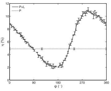
Fig. 8. Plots of efficiency (η) as a function of the phase
ϕ
[6]. P+L and P indicate, respectively, when the biaxial mode and the single mode are used
3.- RESEARCH OBJECTIVES AND APPROACH
The overall purpose of developing the biaxial driving technique is to increase the acoustic efficiency on piezoelectric transducers. These results will lead to evaluate the use of the biaxial method for ultrasound imaging as well as the possibility to use different types of piezoelectric materials with low piezoelectric properties. More specifically, the following questions are being answered:
- Is the acoustic efficiency on a biaxial mode transducer greater than the efficiency on a single mode transducer?
- What are the parameters that govern the biaxial driving effect?
- Could be an array of biaxial transducers be applied to ultrasound imaging?
- Is there any advantage of using, on ultrasound imaging, an array of biaxial transducers over the conventional imaging probes?
- Besides PZT, which other piezoelectric material would be enhanced while using the biaxial driving technique?
There are three major phases on this research project. Phase one correspond to the fabrication and characterization of single element PZT biaxial transducers to compare the acoustic efficiency with single mode transducers. Phase two is to design and characterize an array of biaxial transducers to be applied on ultrasound imaging. Phase three involves the design, fabrication and characterization of biaxial transducers made with materials different than PZT. The biaxial effect has been demonstrated [6] but the overall acoustic efficiency showed on those transducers was low. I hope to gain insight on the biaxial effect and to improve the overall acoustic efficiency on biaxial transducers.
3.1 Research methodology
To probe that the acoustic efficiency produced by the biaxial driving technique is greater than the one on single mode transducers, the fabrication and characterization of single element biaxially driven transducers made of PZT is proposed. The single element structure allows to drive transducers on a simple way, by only using a signal generator and an amplifier per mode. PZT is one of the most widely used piezoelectric materials and with the highest piezoelectric properties.
The difference in phase of the propagation and lateral mode has been demonstrated [6] to have considerable repercussions on the acoustic efficiency response. To establish what other parameters have an impact on the acoustic efficiency of biaxial transducers, a frequency and power sweep are proposed.
To drive an array of biaxial transducers for ultrasound imaging, the number of generators and amplifiers is equal to twice the number of elements on the array. Having these numbers of equipments is not feasible, so to drive this array, the use of the Vantage platform from Verasonics is proposed. This system allows to drive of up to 128 elements at the same time and processing the signals for ultrasound imaging applications if necessary. To ensure that the biaxial transducer array is working the same way as the single element biaxial transducer, the acoustic pressure as a function of the relative phase on the lateral mode needs to be measured by using a hydrophone. The acoustic pressure of the array has to have a sinusoidal response as a function of the phase.
4.- CURRENT WORK
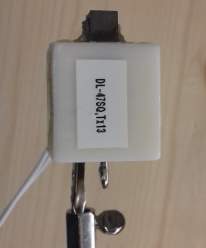
Is important to note that there are three generations of biaxial transducers. The first set of transducers (G1) correspond to a set of three ring shaped biaxial transducers which were developed and characterized on [6]. A second generation of transducers (G2) correspond to a set of three rectangular shaped biaxial transducers which were characterized but not manufactured on this work. The third generation of biaxial transducers (G3) correspond to a set of eight rectangular shaped biaxial transducers which were both, manufactured and characterized on this work. The differences between second and third generation of biaxial transducers are the electrode material and the addition of silver epoxy on the soldering point of the electrodes. Fig. 9 shows one of each generation of biaxial transducers.
- (b) (c)
Fig. 9 (a) Ring shape biaxial transducer from the first generation. (b) and (c) Rectangular shape biaxial transducer from the second and third generation of transducers.
4.1 Biaxial transducer manufacturing process
Eight biaxial transducers were custom built using hard lead zirconate titanate (PZT) (DL47, DeL Piezo Specialities, LLC, West Palm Beach, FL, USA) with a rectangular geometry 6.4 mm x 6.4 mm x 13.7 mm. The geometrical dimensions were set so that the resonant frequency for the propagation and the lateral mode was as close as possible to get the best power conversion [6]. The transducers were built air-backed using a 3D-printed custom ABS casing (Taz 5, Lulzbot, Colorado, USA) in two parts which were assembled using epoxy glue (301, epoxy technology, Billerica, MA) and silicone (Silicone I*, Momentive performance materials Inc., NC, USA). A drop of silver epoxy (8331S-15G, MG Chemicals, B.C., Canada) was used to strengthen the solder joint at each pair of electrodes. A schematic drawing of the transducer is displayed in Fig. 10.
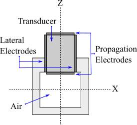
Fig. 10. Cross-section of a 6.4 mm x 6.4 mm x 1.7mm biaxial ultrasound transducer. Electrodes correspond to the propagation (P) and lateral (L) mode of the transducer. The transducers were poled along the propagation direction.
Due the fact that the power amplifiers have an output impedance equal to 50 Ω, both, propagation and lateral electrodes, were matched to 50 Ω at their respective resonant frequency using a transformer matching. The impedance characterization for each mode was done using a vector network analyzer (87511A, Hewlett Packard, Kobe Instruments Division, Hyogo, Japan).
4.2 Biaxial transducer efficiency characterization
A set of fourteen transducers were characterized, three ring shaped transducers from the 1st generation, three rectangular transducers from the 2nd generation of biaxial transducers and eight rectangular transducers from the 3rd generation of biaxial transducers.
The acoustic power of the transducers was characterized using the radiation force method [44]. This method establish that a change of mass on an absorber is proportional to the amount of acoustic power delivered for an ultrasonic transducer. A change in mass that can be measured by using an analytical scale. A 6-cm diameter cylindrical absorber (HAM A, Precision Acoustics, Dorchester, Dorset, UK) was placed at the bottom of a container filled with deionized-degassed water, placed on top of an analytical scale (PI-225D, Denver Instrument, Bohemia, NY, USA). The ultrasound transducer was placed 2-cm away from the absorber and the ultrasound beam was directed vertically downward to the target. Continuous sinusoidal signals from a dual-channel function generator (33522A, Agilent Technologies, Santa Clara, CA) were used to drive independently each mode (P and L). Signals were amplified independently (AG 1021, T&C Power Conversion, Rochester, NY and 240L, E&I, Rochester, NY) and each acquisition tested a phase shift
ϕ
relative to the P-electrode from 0° to 360° (randomly selected) at a 10° resolution.
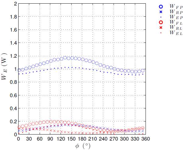
A -30 dB dual directional coupler (C10241-10, Werlatone, Patterson, NY) was used on each mode to get a signal sample. The electrical power was measured with two power meters (N1914A & E4419B, Agilent Technologies, Santa Clara, CA) with its respective sensors (N8482H, Agilent Technologies, Santa Clara, CA) for lateral and propagation mode respectively. Due the fact that the water container is small, evaporation was observed during the measurements and a mass compensation was applied [6]. All the acquisitions were performed using a laptop computer (Lattitude E6500, Core 2 P8600 at 2.4 GHz, 4 GB RAM, Dell Computers, Round Rpck, TX) running in-house control programs in Matlab R2009 (Mathworks, Natick, MA). Fig. 11 represents the efficiency characterization setting.
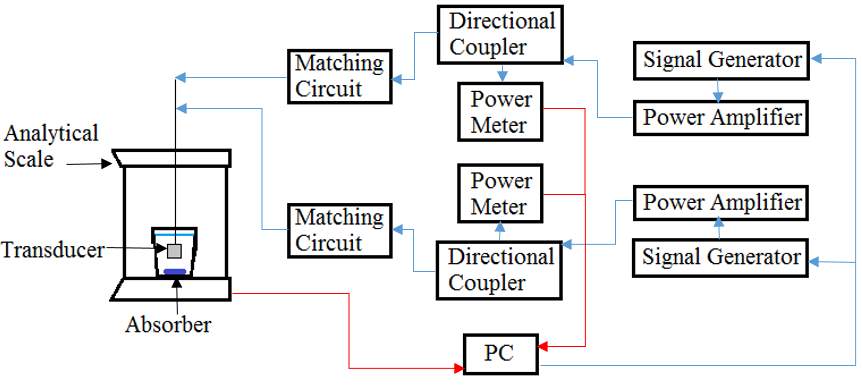
Fig. 11. Efficiency characterization schematic. Red lines represent information transmitted to the computer.
To achieve the best acoustic efficiency with the biaxial driving technique, two major set of experiments were done: Frequency sweep and power variation.
4.3 Frequency sweep experiments
Due the fact that the resonant frequency on the lateral and propagation mode is not exactly the same, is hard to tell what frequency on each mode produces the best efficiency. The purpose of this set of experiments is to establish what frequency, applied on the lateral and propagation modes, produces a better acoustic efficiency. As can be seen on the first generation of biaxial transducers [6], using the individual resonant frequency on each mode produces the worst results. Three different sets of frequencies for both modes were tested, the resonant frequency of propagation mode (F1), the resonant frequency of lateral mode (F2) and the average of those resonant frequencies (AVG). The characterization procedure described on section 4.2 was used to measure the acoustic efficiency in dependence of
ϕ
. A series of three set of measurements were done on each transducer.
For each combination of
ϕ
, the power efficiency (η) and the electrical power (reflected and forward) was measured. The acoustic power [44]
WA
was calculated as a function of
ϕ
given by
| WAϕ=mϕgc
, |
(32) |
where
m(ϕ)
is the change of mass (kg) measured using the analytical scale after eight seconds of continuous driving of the transducer, g is the gravity constant (9.81 ms-2) and c is the speed of sound in water (1481 ms-1) at room temperature. The power efficiency η(
ϕ
) was calculated with [44]
| ηϕ=WA(ϕ)WE(ϕ)×100%, | (33) |
Where
WEϕ=WEPϕ+WEL(ϕ)
is the effective electrical power (forward minus reflected) on both electrodes,
WEP
is the effective power measured for the propagation mode and
WEL
is the effective power measured for the lateral mode. The power was configured to deliver 1 effective W on each mode, for a total of 2 W. To compare the efficiency gain of the biaxial mode with respect to the single mode, acquisitions were done driving only the P-electrode with
WEϕ=2 W
. This configuration was used to compare the biaxial mode to single mode (baseline). A set of three first generation biaxial transducers and nine second generation transducers were tested.
4.4 Power variation experiments
It was proposed that the amount of power delivered to the lateral mode do not need to be the same magnitude as the propagation mode, but a fraction of it. For these experiments, the P-electrode received a constant electrical power of 1 W while the L-electrode power was varied. Each experiment combination tested a phase shift
ϕ
relative to the P-electrode and a different value of power for the L-electrode. The power applied on the L-electrode was a fraction of the power applied on the P-electrode. This fraction is referred as the power ratio Pr. The phase shift was changed from 0° to 360° with a 10° resolution and the values of Pr were 0.1, 0.25, 0.5, 0.75, and 1 for the first and third generation transducers and 0.13, 0.33, 0.66 and 1 for the second generation of transducers. The characterization procedure described on section 4.2was used to measure the acoustic efficiency in dependence of
ϕ
and Pr. Three ring shaped biaxial transducers, three second generation transducers and eight third generation transducers were tested driving both, lateral and propagation mode, with the average of their resonant frequencies. A series of three set of measurements were done on each transducer.
The acoustic power [44]
WA
was calculated as a function of
ϕ
for each Pr and it is given by
| WAϕ,Pr=mϕ,Prgc
, |
(34) |
where
m(ϕ,Pr)
is the change of mass (kg) measured using the analytical scale after eight seconds of continuous driving of the transducer, g is the gravity constant (9.81 ms-2) and c is the speed of sound in water (1481 ms-1) at room temperature. The power efficiency η(
ϕ,Pr
) was calculated with [44]
| ηϕ,Pr=WA(ϕ,Pr)WE(ϕ,Pr)×100%, | (35) |
where
WEϕ,Pr=WEPϕ+WEL(ϕ,Pr)
is the effective electrical power (forward minus reflected) on both electrodes,
WEP
is the effective power measured for the propagation mode and
WEL
is the effective power measured for the lateral mode. To compare the efficiency gain of the biaxial mode with respect to the single mode, acquisitions were done driving only the P-electrode with the average frequency, using
WEϕ,Pr=WEPϕ=2 W
or 1.5 W for the second generation of transducers. This configuration was used to compare the biaxial mode to single mode (baseline).
5.- PRELIMINARY RESULTS
Table 2 shows the electrical characterization results. The global average (± s.d.) for the first, second and third generation of biaxial transducers, respectively, is 491.3 (± 8.2) kHz, 138.7 (± 0.7) kHz and 135.5 (± 0.31) kHz. Table 3 shows the results from the frequency sweep characterization. From the six transducers tested, three of them presented a highest acoustic efficiency when using the average frequency on both, three of them when using propagation frequency and none of them when using lateral frequency on both modes. This results indicate that, in general, the lowest maximum acoustic efficiency was reached when both modes were driven by using the lateral resonant frequency, and that the transducers tend to have a better response when average or propagation frequency is used on both. Table 4 summarize the results of the power variation experiments showing the η values of the baseline and the maximum η reached, including the relative phase and the power ratio where it was reached. To compare results, the values of each transducer with a Pr = 1 were included. There was an overall gain of 3.87 % (± 2.27 %) when comparing the maximum η and the η at a Pr = 1 and an overall gain of 3.62 % (± 2.36 %) when compared to the baseline. Fig. 12 shows the acoustic efficiency vs. relative phase plot for a Pr = 1 and the Pr where the maximum η was reached for one of each generation of transducers.
TABLE 2
Resonant Frequency
| TX | Resonant Frequency P-mode | Resonant Frequency L-mode | Difference between frequencies (|P-L|) | Average Frequency |
| G11 | 494.972 | 473.77 | 21.202 | 484.371 |
| G12 | 503.525 | 497.05 | 6.475 | 500.2875 |
| G13 | 491.912 | 486.475 | 5.437 | 489.1935 |
| G21 | 136.525 | 142.45 | 5.925 | 139.4875 |
| G22 | 137.462 | 139.017 | 1.555 | 138.2395 |
| G23 | 135.687 | 141.262 | 5.575 | 138.4745 |
| G31 | 133.3 | 138.3 | 5.3 | 135.65 |
| G32 | 133 | 137.5 | 4.5 | 135.25 |
| G33 | 132.4 | 138 | 5.6 | 135.2 |
| G34 | 133 | 138.5 | 5.5 | 135.75 |
| G35 | 133.3 | 137.6 | 4.3 | 135.45 |
| G36 | 133.3 | 138.5 | 5.2 | 135.9 |
| G37 | 132.5 | 137.5 | 5 | 135 |
| G38 | 133.3 | 138.9 | 5.6 | 135.65 |
TABLE 3
Frequency Characterization Results
| TX | Frequency mode | Freq. P (kHz) | Freq. L (kHz) | Baseline (n%) | Max η (%) | φ | Min η (%) | φ |
| G11 | F1 | 494.972 | 494.972 | 29.64 | 26.08 | 37 | 21.66 | 197 |
| G11 | F2 | 473.77 | 473.77 | 19.64 | 22.81 | 22 | 16.66 | 207 |
| G11 | AVG | 484.371 | 484.371 | 26.23 | 26.33 | 37 | 20.16 | 187 |
| G12 | F1 | 503.525 | 503.525 | 32.31 | 33.54 | 62 | 25.55 | 242 |
| G12 | F2 | 497.05 | 497.05 | 34.35 | 34.25 | 57 | 26.81 | 207 |
| G12 | AVG | 500.287 | 500.287 | 34.01 | 34.45 | 72 | 26.55 | 222 |
| G13 | F1 | 491.912 | 491.912 | 31.66 | 33.75 | 182 | 22.75 | 2 |
| G13 | F2 | 486.475 | 486.475 | 30.95 | 32.69 | 167 | 21.42 | 327 |
| G13 | AVG | 489.193 | 489.193 | 30.45 | 31.91 | 147 | 22.33 | 352 |
| G21 | F1 | 136.525 | 136.525 | 34.06 | 23.32 | 232 | 20.26 | 47 |
| G21 | F2 | 142.45 | 142.45 | 17.35 | 16.14 | 292 | 14.15 | 327 |
| G21 | AVG | 139.487 | 139.487 | 27.48 | 20.12 | 232 | 16.84 | 77 |
| G22 | F1 | 137.462 | 137.462 | 19.88 | 18.18 | 207 | 11.69 | 42 |
| G22 | F2 | 139.012 | 139.012 | 16.86 | 17 | 207 | 10.88 | 62 |
| G22 | AVG | 138.237 | 138.237 | 18.23 | 17.78 | 217 | 11.51 | 67 |
| G23 | F1 | 135.687 | 135.687 | 22.03 | 15.68 | 27 | 10.97 | 162 |
| G23 | F2 | 141.262 | 141.262 | 14.47 | 13.98 | 42 | 8.01 | 257 |
| G23 | AVG | 138.474 | 138.474 | 18.53 | 15.69 | 22 | 9.89 | 202 |
TABLE 4
Power Variation Results
| TX | Baseline (η%) | ϕ
(deg) |
η (%) at Pr 1 | Max η (%) | ϕ
(deg) |
Reached at Pr |
| G11 | 31.11 | 12 | 29.3 | 32.95 | 32 | 0.25 |
| G12 | 27.71 | 72 | 28.28 | 31.09 | 32 | 0.25 |
| G13 | 31.01 | 192 | 31.62 | 37.16 | 182 | 0.25 |
| G21 | 29.49 | 232 | 20.56 | 29.25 | 242 | 0.13 |
| G22 | 18.99 | 232 | 19.14 | 20.7 | 222 | 0.13 |
| G23 | 21.21 | 52 | 16.9 | 24.21 | 52 | 0.13 |
| G31 | 21.32 | 0 | 20.11 | 23.81 | 0 | 0.1 |
| G32 | 22.57 | 30 | 19.32 | 23.77 | 40 | 0.1 |
| G33 | 18.24 | 260 | 16.96 | 20.59 | 300 | 0.1 |
| G34 | 18.46 | 60 | 23.41 | 25.15 | 70 | 0.25 |
| G35 | 19.27 | 70 | 25.54 | 26.5 | 70 | 0.5 |
| G36 | 19.67 | 60 | 24.75 | 26.29 | 70 | 0.25 |
| G37 | 21.82 | 310 | 18.35 | 24.68 | 270 | 0.1 |
| G38 | 20.2 | 240 | 23.39 | 25.62 | 250 | 0.25 |
| η AVG (±s.d.) | 22.93 (± 4.76) | 22.69 (± 4.71) | 26.56 (± 4.63) |
(a)
(b)
(c)
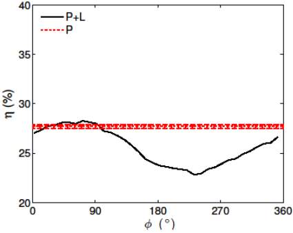
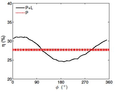
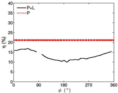
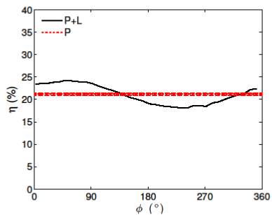
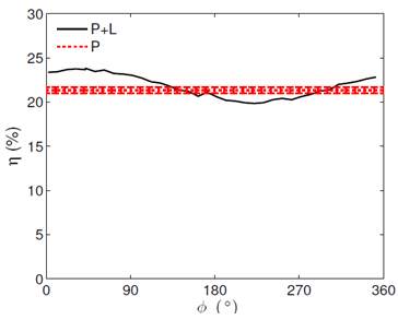
Fig. 12. Plots of efficiency as a function of the phase η(
ϕ) for (a) the first generation biaxial transducer G12 (b) the second generation biaxial transducer G23 (c) the third generation biaxial transducer G31. (a) Pr = 1 and Pr = 0.25. (b) Pr = 1 and Pr = 0.13. (c) Pr = 1 and Pr = 0.1 respectively. P+L and P indicate, when the biaxial mode and the single mode are used.
5.1 Power efficiency vs. Electrical power
Fig. 13 displays a typical efficiency vs. phase plot and its electrical response. It is worth noting the sinusoidal response of the efficiency and electrical response are both a function of
ϕ
. Because of this observation, we evaluated the possibility of correlating the value of
ϕ
for the maximum efficiency with the electrical response.
For this purpose, a sinusoidal fitting was applied to all the third generation biaxial transducer measurements (efficiency and electrical) from the power variation experiments. The value of
ϕ
where each the forward, reflective and effective electrical power was maximal was correlated to the value of
ϕ
where efficiency η was maximal. The following linear regression was applied
| yi=β0+β1xi
, |
(36) |
with
yi
representing the value of
ϕ
at which the maximum power efficiency is achieved,
β0
and
β1
are the intercept and slope coefficients and
xi
is the predictor. We also obtained the residuals
ri
as the difference between the observed values
yi
and the estimated values
yî
[45].
Table 5 summarize the linear regression results. The linear regression analysis was done using R version 3.3.1 (R Core Team (2016), Vienna, Austria). To work on the region where the biaxial mode has higher η than single mode, the maximum absolute value for the residual needs to be less than 90 ° so that
ϕ
is in the positive region of the efficiency response (Fig. 13b) for all transducers. It was observed that the measurement of the reflected power on the L-electrode was the best predictor overall, with a linear regression R2 value increasing and a residual value decreasing when Pr is decreased, having a Pr of 0.1 as the best regression. Fig. 14 shows the scattering and linear regression plot of the reflected power response on the L-electrode with a Pr of 0.1. The observed, estimated and residual values can be found on Table 6.
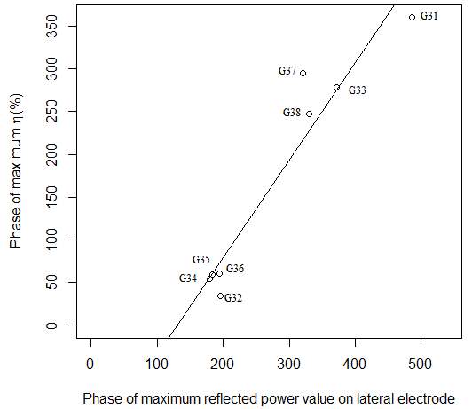
Fig. 14. Scattering and linear regression plot of the difference in phase (deg) at which the maximum power efficiency is obtained using the biaxial mode vs. the difference in phase (deg) at which the maximum value of the reflected power on lateral electrode is obtained when using a power ratio of 0.1. R2 = 0.92.
(a)
(b)
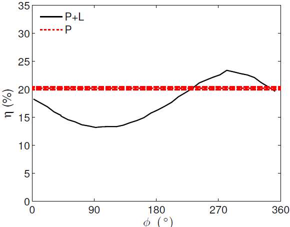
Fig. 13. Plots of efficiency as a function of the phase η(
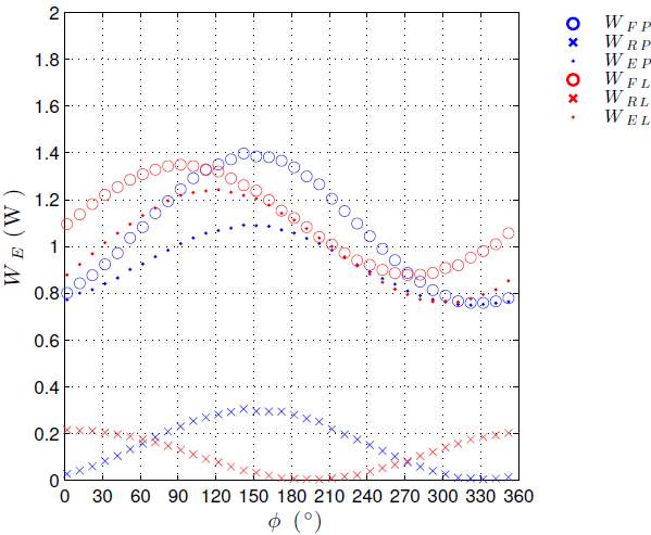
ϕ) and the corresponding electrical power for transducer G38. (a) Pr = 1. (b) Pr = 0.1. P+L and P indicate, respectively, when the biaxial mode and the single mode are used. WF, WR and WE represent, respectively, the forward, reflected and effective power on each electrode (P or L).
TABLE 6
Best Predictor Results
| TX | Observed phase (deg) for max η(%) | Estimated phase (deg) for max η(%) | |ri| |
| G31 | 359.79 | 44.61 | 44.82 |
| G32 | 34.71 | 74.87 | 40.16 |
| G33 | 278.25 | 275.11 | 3.14 |
| G34 | 54.30 | 56.86 | 2.56 |
| G35 | 59.79 | 60.97 | 1.18 |
| G36 | 60.76 | 72.75 | 11.99 |
| G37 | 294.46 | 216.82 | 77.64 |
| G38 | 247.44 | 227.49 | 19.95 |
The estimated and residual values for the difference in phase (deg) at which the maximum power efficiency on biaxial mode is obtained vs. the difference in phase (deg) at which the maximum value of the reflected power response on the lateral electrode at a power ratio of 0.1
TABLE 5
Linear Regression of Phase for Maximum Between Electrical Power and Efficiency
| Power ratio 1 | Power ratio 0.75 | Power ratio 0.5 | ||||||||||
| Predictors | R2 | β0̂ | β1̂ | Highest |Residual| | R2 | β0̂ | β1̂ | Highest |Residual| | R2 | β0̂ | β1̂ | Highest |Residual| |
| PF | 0.36 | -294.39 | 1.30 | 168.95 | 0.31 | -256.69 | 1.20 | 170.78 | 0.33 | -265.95 | 1.22 | 162.37 |
| PE | 0.35 | -244.58 | 1.18 | 175.45 | 0.31 | -215.05 | 1.10 | 177.90 | 0.32 | -220.83 | 1.12 | 179.41 |
| PR | 0.51 | -300.16 | 1.226 | 157.77 | 0.39 | -218.74 | 1.02 | 123.88 | 0.42 | -226.46 | 1.05 | 129.07 |
| LF | 0.06 | -35.24 | 0.66 | 139.41 | 0.05 | -34.00 | 0.65 | 141.87 | 0.05 | -26.94 | 0.63 | 143.79 |
| LE | 0.06 | 4.44 | 0.50 | 142.46 | 0.07 | -1.16 | 0.51 | 143.62 | 0.07 | 5.62 | 0.49 | 145.65 |
| LR | 0.20 | 21.87 | 0.46 | 130.92 | 0.91 | -145.01 | 1.110 | 87.39 | 0.9 | -140.31 | 1.1 | 86.84 |
(a)
| Power ratio 0.25 | Power ratio 0.1 | |||||||
| Predictors | R2 | β0̂ | β1̂ | Highest |Residual| | R2 | β0̂ | β1̂ | Highest |Residual| |
| PF | 0.33 | -262.11 | 1.22 | 163.00 | 0.30 | -238.73 | 1.16 | 163.25 |
| PE | 0.31 | -202.56 | 1.07 | 176.04 | 0.29 | -191.50 | 1.05 | 176.59 |
| PR | 0.59 | -316.83 | 1.26 | 170.71 | 0.42 | -220.33 | 1.03 | 130.25 |
| LF | 0.05 | -20.67 | 0.61 | 143.59 | 0.04 | 14.79 | 0.50 | 143.49 |
| LE | 0.05 | 33.72 | 0.41 | 148.37 | 0.05 | 46.86 | 0.37 | 147.22 |
| LR | 0.92 | -141.67 | 1.11 | 78.04 | 0.92 | -148.05 | 1.14 | 77.64 |
(b)
Linear regression results for all predictors. (a) Power ratios 1, 0.75 and 0.5. (b) Power ratios 0.25 and 0.1. P and L indicates, respectively, P-electrode and L-electrode. F, E and R indicates the forward, effective or reflected power.
The results from varying the phase shift and power for the third generation transducers (Table 4) show that the value of phase
ϕ
at which the maximum power efficiency is obtained remains constant independently of the amount of power applied to the lateral electrode (Fig. 15). The standard deviation values of the phase at each power ratio varied depending on the transducer between 0 (G31) to 17.9 (G38) degrees. Some of these variations are explained due the 10° resolution of the acquisition. As shown in Table 5, the highest power efficiency was reached when using a power ratio between 0.1 to 0.5, an important fact that shows that reducing the amount of electrical power delivered to the lateral mode of the transducer is more advantageous to increasing efficiency, as it is seen on Fig. 16. This observation indicates that, when using biaxial driving, only a fraction of the energy applied to the propagation electrode needs to be applied to the lateral electrode at the proper phase to produce the increase in efficiency reported for this driving. The analysis showed that there were four transducers with a low power efficiency gain over baseline when compared to the others. This reduced efficiency was correlated to the coefficient of determination (R2) on the electrical power curves after the sinusoidal fitting, as shown in Table 7. If one or more of the fitted electrical power curves (forward, effective or reflected power in either electrode) present a R2 less than 0.9, the power efficiency gain of the biaxial transducer will be close or even inferior to the baseline. However, this can be avoided by using low values of Pr. The use of low values of Pr have important implications in the fabrications as the electronics driving L-electrodes will require less power (close to 1 order of magnitude). Fig. 17 shows the maximum gain on efficiency (max biaxial η / baseline η) for every power ratio.
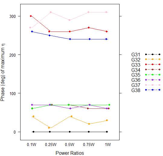
Fig. 15. The phase at which the maximum efficiency η(
ϕ
) was found for each transducer at every tested power ratio.
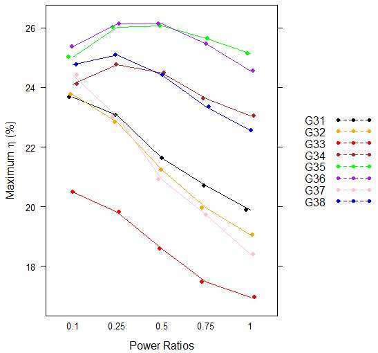
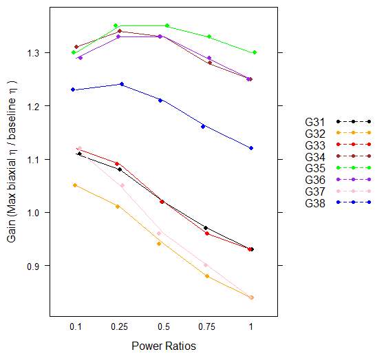
Fig. 16. Different η(
%
) for each transducer at Fig. 17. Biaxial gain for each transducer at
every tested power ratio. every tested power ratio
6.- WORK PLAN
| Year 1 | Year 2 | Year 3 | |
| Course work | |||
| Background research | |||
| Development of single element biaxial transducers | |||
| Development of matching network for single element biaxial transducers | |||
| Characterization of acoustic efficiency relative to frequency and phase on both modes of a biaxial transducer | |||
| Characterization of acoustic efficiency relative to power and phase on both modes of a biaxial transducer | |||
| Writing a paper with the results (Ultrasonics – Journal – Elsevier) | |||
| Design of arrays of biaxial transducers | |||
| Characterization of the acoustic pressure of a the arrays of biaxial transducers | |||
| Application of the arrays of biaxial transducers on ultrasound imaging | |||
| Writing a paper with the results (IEEE Transaction on Ultrasonics, Ferroelectrics and Frequency Control) | |||
| Development of single element biaxial transducers with other materials | |||
| Writing a paper with the results (Ultrasonics – Journal – Elsevier) | |||
| Comprehensive examination | |||
| PhD Seminar | |||
| PhD Dissertation |
7.- CONCLUSIONS
The feasibility of applying the biaxial driving technique to piezoelectric materials was presented on this work with the purpose of increasing the overall acoustic efficiency. This technique consist on applying two dephased orthogonal electrical fields to a piezoelectric actuator. In this research work, a total of fourteen biaxial transducers were characterized by using a radiation force system to calculate the acoustic efficiency relative to the phase and power delivered to both modes. The results reveal an overall reduction on power consumption in comparison to single mode due the fact that a higher efficiency was reached when only a fraction of the power that is used on the propagation electrode needs to be applied to the lateral electrode on biaxial mode transducers. The results indicates that with the proper phase and power, a single element PZT transducer driven biaxially can increase its efficiency up to 37.5% when compared to applying a single electrical field in the pole direction. A method to calculate the optimal phase at which a PZT ultrasound transducer that is driven biaxially will present maximum efficiency was also presented on this work. The relationship of the electrical input power on both electrodes and the maximum efficiency will allow using only the electrical response of the transducer to determine the best driving conditions. This will translates into a reduced time of characterization since acoustic power measurements can be avoided. Also, it was found that a way to measure the effectiveness of the biaxial driving technique on a given transducer can be based on the analysis of the coefficient of determination on the fitting of electrical input power curves.
REFERENCES
[1].- Stranford G, Vencill T, Williams D, Johnson B, Gutierrez L (2014) Piezoelectric ceramics in ultrasound, presented at 2014 IEEE International Ultrasonics Symposium (IUS), Chicago, USA. 2014. Published by IEEE. doi: 10.1109/ULTSYM.2014.0220
[2].- Shi G, Chen J, Qi Y, Yu S, Cheng J (2009) Dielectric and piezoelectric enhancements in the BiFeO3-PbTiO3 solid solutions with Gd doping, presented at 18th IEEE International Symposium on the Applications of Ferroelectrics, Xian, China. 2009. Published by IEEE. doi: 10.1109/ISAF.2009.5307560.
[3].- Ali A, Ahn C, Kim Y (2013) Enhancement of piezoelectric and ferroelectric properties of BatiO3 ceramics by aluminum doping. Ceramics International 39, 6623-6629. http://dx.doi.org/10.1016/j.ceramint.2013.01.099.
[4].- Wang CM, Wang JF, Gai ZG (2007) Enhancement of dielectric and piezoelectric properties of M0.5Bi4.5Ti4O15 (M = Na, K, Li) ceramics by Ce doping. Scripta Materialia 57, 789-792. http://dx.doi.org/10.1016/j.scriptmat.2007.07.015.
[5].- Cheung K, Zhou D, Lam K, Chen Y, Dai J (2011) Performance enhancement of a piezoelectric linear array transducer by half-concave geometric design. Sensors and Actuators A Physical 172(2). doi: 10.1016/j.sna.2011.09.035.
[6].- Pichardo S, Silva RRC, Rubel O, Curiel L (2015) Efficient Driving of Piezoelectric Transducers Using Biaxial Driving Technique. PLoS ONE 10(9): e0139178. doi:10.1371/journal.pone.0139178.
[7].- Fu H, Cohen RE (2000) Polarization rotation mechanism for ultrahigh electromechanical response in single-crystal piezoelectrics. Nature 403, 281-283. doi:10.1038/35002022.
[8].- Budimir M, Damjanovic D, Setter N (2007) Qualitative distinction in enhancement of the piezoelectric response in PbTiO3 in proximity of coercive fields: 90° versus 180° switching. Journal of applied physics 101, 104119. doi: 10.1063/1.2733594.
[9].- Cole J, Ahmed S, Curiel L, Pichardo S, Rubel O (2014) Marble game with optimal ferroelectric switching. Journal of Physics: Condensed Matter 26, 135901 (9pp). doi: 10.1088/0953-8984/26/13/135901.
[10].- M. I. Gutiérrez, “Modelado del calentamiento de radiación acústica generada por equipos de fisioterapia ultrasónica, validación experimental en medios homogéneos y diseño de la instrumentación”, in Department of Electrical Engineering. Doctoral Thesis. México, D.F.: CINVESTAV-IPN, 2011.
[11].- S. A. Delgado, “Dispositivo portátil para la excitación de transductores HIFU monoelemento y monitoreo de su acoplamiento mediante la medición de la relación de onda estacionaria”, in Department of Electrical Engineering. Master Thesis. México, D.F.: CINVESTAV-IPN, 2015.
[12].- Cobbold, R. S. (2007). Foundations of biomedical ultrasound. New York, NY: Oxford University Press, Inc.
[13].- Repacholi, M. H., Grandolfo, M., Rindi, A. (1987). Ultrasound. Medical applications, biological effects and hazard potential. New York, NY:Plenum Press.
[14].- A. Carovac, F. Smajlovic and D. Junuzovic, “Application of Ultrasound in Medicine ”, Acta Informatica Medica. 19(3), 2011.
[15].- P. Patil and B. Dasgupta, “Role of diagnostic ultrasound in the assessment of muscoeskeletal disease ”, Therapeutic Advances in Muscoeskeletical Disieses. 4(5), 2012.
[16].- D. Miller, N. Smith, M. Bailey, G. Czarnota, G. Hynynen, K. Makin and American Institute of Ultrasound in Medicine Bioeffects Committe “Overview of Therapeutic Ultrasound Applications and Safety Considerations ”, Journal of Ultrasound in Medicine: Official Journal of the American Institute of Ultrasound in Medicine, 31(4), 2012.
[17].- S. Mitragotri “Healing sound: the use of ultrasound in drug delivery and other therapeutic applications ”, Nature Reviews Drug Discovery, 4(3), 2005.
[18].- C. Tempany, E. Stewart, N. McDannold, B. Quaude, F. Joles and K. Hynynen, “MR imaging-guided focused ultrasound surgery of uterine leiomyomas: a feasibility study ”, Radiology, 226(3), 2003.
[19].- U.S. Food and Drug Administration, Center for Devices and Radiological Health (CDRH). “ExAblate Model 4000 Type 1.0 System (ExAblate Neuro) for the unilateral Thalamotomy treatment of idiopathic Essential Tremor patients with medication refractory tremor”, Approval letter, July 11th, 2016. https://www.accessdata.fda.gov/cdrh_docs/pdf15/P150038a.pdf.
[20].- U.S. Food and Drug Administration, Center for Devices and Radiological Health (CDRH). “ExAblate System, Model 2000/2100/2100 V1 for pain palliation of Metastatic Bone Cancer”, Approval letter, October 18th, 2012. https://www.accessdata.fda.gov/cdrh_docs/pdf11/P110039A.pdf.
[21].- U.S. Food and Drug Administration, Center for Devices and Radiological Health (CDRH). “Sonablate® 450 indicated for transrectal high intensity focused ultrasound (HIFU) ablation of prostatic tissue”, Approval letter, October 9th, 2015. https://www.accessdata.fda.gov/cdrh_docs/pdf15/DEN150011.pdf.
[22].- M. Ghorbani, O. Oral, S. Eckini, D. Gozuacki and A. Kozar, “Review on Lithotripsy and Cavitation in Urinary Stone Therapy”, IEEE Reviews in Biomedical Engineering, 9(6), 2016.
[23].- Hill, C. R., Bamber, J. C., ter Harr, G. R. (2004). Physical principles of medical ultrasonics. West Sussex, UK. John Wiley & Sons Ltd.
[24].- Laughier, P., Haiat, G. (2011). Bone quantitative ultrasound. Dordrecht, Germany: Springer.
[25].- J. L. Teja, “Diseño de un dispositivo para Hemostasia Acústica con Ultrasonido Focalizado de Alta Intensidad mediante simulaciones FEM”, in Department of Electrical Engineer. Master Thesis. México, D.F.: CINVESTAV-IPN, 2013.
[26].- Pierce, A. D. (1994). Acoustics. An introduction to its physical principles and applications. Melville, NY: Acoustical society of America.
[27].- P. Curie and J. Curie, “Développement par presion de l’electricité polaire dans les cristaux hémiedres a faces enclinés,” Compt. Rendus, 91, 383, 188.
[24].- Nimrod, M. (2005). Basic physics of ultrasonographic imaging. Geneva, Switzerland. World Health Organization.
[29].- Lippman, G. (1881). “Principe de la conservation de l’électricité”, Annales de chimie et de physique 24:145.
[30].- Boston Piezo Optics Inc. Intro to piezoelectric transducer crystals. Bellingham, MA, USA.
[31].- S. J. Ahmed, “Computer simulation of functional materials for therapeutic ultrasound applications”, Department of physics. Master thesis. Thunder Bay, ON, Canada. Lakehead University, 2013.
[32].- APC International, Ltd. Piezoelectric ceramics principles and applications.
[33].- B. Jaffe, R. S. Roth and S. Marzullo, “Piezoelectric properties of lead zirconate – lead titanate solid solution ceramic ware”, J. Appl. Phys., 25, 1954.
[34].- Safari, A., Koray, E., (2008). Piezoelectric and acoustic materials for transducer applications. New York, NY: Springer.
[35].- B. E. Eovino, “Design and analysis of a PVDF Acoustic Transducer Towards an Imager for Mobile Underwater Sensor Networks”, in Department of Electrical Engineering and Computer Science. Technical report. USA, Californa, Santa Barbara.: University of California at Berkeley, 2015.
[36].- T. H. Kim, A. C. Arias, “Characterization and applications of piezoelectric polymers”, in Department of Electrical Engineering and Computer Science. Technical report. USA, Californa, Santa Barbara.: University of California at Berkeley, 2015.
[37].- W. A. Smith, A. A. Shaulov and B. M. Singer (1984) Properties of composite piezoelectric materials for ultrasonic transducers, presented at 1984 IEEE Ultrasonics Sympo. Proc. 1984.
[38].- W. Smith, (1989) The role of piezocomposites in ultrasonic transducers, presented at 1989 IEEE Ultrasonics Sympo. Proc. 1989.
[39].- O. Oralkan, S. Ergun, J. Johnson, M. Karaman, U. Demirci, K. Kaviani, T. Lee, B. Khuri-Yakub, “Capacitive Micromachined Ultrasonic Transducers: Next-Generation Arrays for Acoustic Imaging? ”, IEEE Trans. Ultrason. Ferroelec., Freq. Contr. , 49, 11, 2002.
[40].- S. Wong, M. Kupnik, R. Watkins, K. Butts-Pauly and B. Khuri-Yakub , “Capacitive Micromachined Ultrasonic Transducers for Therapeutic Ultrasound Applications”, IEEE Trans. On Biomedical Engineering, 57,1, 2010.
[41].- M. Sabri, M. F. Abd, R. B. W. Heng, K. Juni, N. Sabri, “Capacitive Micromachined Ultrasonic Transducers: Technology and Application”, Elsevier Journal of Medical Ultrasound., 20, 8-31, 2012.
[42].- G. Haertling, (1999) “Ferroelectric ceramics: History and technology”, Journal of the American Ceramic Society, 82,4,797-818.
[43] H. Fu and R. E. Cohen, “Polarization rotation mechanism for ultrahigh electromechanical response in single-crystal piezoelectrics,” Nature, vol. 403, pp. 281-283, Jan. 2000.
[44].- IEC technical committee 87: Ultrasonics, IEC 61161 Ed. 3.0, 2013, Ultrasonics – Power measurement – Radiation force balances and performance requirements, Geneva.
[45].- Vittinghoff, E., Glidden, D. V., Shiboski, S. C. & McCulloch, C.E. (2012). Regression methods in biostatistics. doi: 10.1000/978-1-4614-1353-0
Cite This Work
To export a reference to this article please select a referencing stye below:
Related Services
View all


Related Content
All TagsContent relating to: "Medical Technology"
Medical Technology is used to enhance the medical care and treatment that patients are given in healthcare settings. Medical Technology can be used to identify, diagnose and treat medical conditions and illnesses.
Related Articles
DMCA / Removal Request
If you are the original writer of this dissertation and no longer wish to have your work published on the UKDiss.com website then please: