Enhancing Disaster Resilience Through Scenario Modelling
Info: 10231 words (41 pages) Dissertation
Published: 8th Jun 2021
Tagged: Geography
Abstract
Studies on how variables of community resilience to natural hazards interact as a system that affects the final resilience, i.e., their dynamical linkages, have rarely been conducted. Bayesian Network (BN), which represents the interdependencies among variables in a graph while expressing the uncertainty in the form of probability distributions, offer an effective way to investigate the interactions among different resilience components and address the natural-human system as a whole. This paper employs a BN to study the interdependencies of 10 resilience variables and population change in the Lower Mississippi River Basin (LMRB) at the census block-group scale. A genetic algorithm was used to identify an optimal BN where population change, a cumulative resilience indicator, was the target variable. The genetic algorithm yielded an optimized BN model with a cross-validation accuracy of 67% over a period of 906 generations. Six variables were found to have direct impacts on population change, including hazard exposure, hazard damages, distance to coastline, employment rate, percent of housing units built before 1970, and percent of households with female householder. The remaining four variables are indirect variables, including percent agriculture land, percent flood zone area, percent owner-occupied house units, and population density. Each variable has a conditional probability table so that its impacts on the probability of population change can be evaluated as it propagates through the network. These probabilities could be used for scenario modeling to help inform policies to reduce vulnerability and enhance disaster resilience.
Keywords: Bayesian network, coupled natural-human system, population change, community resilience, coastal disasters, Lower Mississippi River Basin
1. Introduction
Multiple coastal hazards, including hurricanes, storm surges, flooding, land subsidence, have made coastal communities especially vulnerable. These hazards also have far-reaching impacts on the lives of those affected. (Zou et al., 2015). Due to the spatial variation of the hazard exposure, damages sustained, socioeconomic and environmental characteristics, communities have shown differential behaviors of post-disaster response and recovery (Cutter et al., 2008, 2010; Lam et al., 2015 & 2016; Kumar et al., 2016). These various aspects could be contextualized in the concept ‘community resilience’, which is broadly acknowledged as ‘the ability to prepare and plan for, absorb, recover from and more successfully adapt to adverse events’ (Lam et al., 2016; NRC, 2012). Community resilience is a multifaceted concept, which is shaped over time through the interactions within several dimensions including social, economic, natural and environmental (Norris et al., 2008; Joerin et al., 2012).
Substantial effort has been made to identify variables and develop frameworks to measure community resilience, which is the first and fundamental step towards understanding resilience (NRC, 2012; Cutter et al., 2008). The Baseline Resilience Indicators for Communities (BRIC) integrated six dimensions to comprehensively assess community resilience. The six dimensions include social, infrastructural, economic, institutional, community, and environmental (Cutter et al., 2010 & 2014). The Resilience Inference Measurement (RIM) framework aims to overcome the challenge of empirical validation of resilience index through k-means clustering of communities’ behaviors before, during, and after disasters and discriminant analysis of influencing factors from multiple resilience dimensions (Lam et al., 2015, 2016; Cai et al., 2016). Other resilience indices examples include Coastal Resilience Index created by National Oceanic and Atmospheric Administration (NOAA, 2010), PEOPLES Resilience Framework (Renschler et al., 2010), the Communities Advancing Resilience Toolkit (CART) (Pfefferbaum et al. 2011), and the community assessment of resilience tool (NRC, 2012).
However, few studies have progressed beyond static measurement of resilience into dynamics of resilience by quantifying the interactions among different components. To better understand disaster resilience, we must consider the complex dynamics among the various factors (Schultz and Smith, 2016). However, modeling the dynamics of resilience have many challenges. First, existing resilience assessment research often find it difficult to include indicators from both natural and human systems, which are necessary to understand the interdependencies among the social and environmental aspects of resilience (Qiang and Lam, 2016). Difficulties arise from various technical issues, such as data availability and data compatibility between the natural and human variables. Second, empirical validation of a resilience index has been a major issue in static resilience measurement research (Burton, 2015; Tate, 2012; Lam et al., 2015; Bakkensen et al., 2016). The same issue also applies to dynamic resilience analysis where the relationships between different resilience components need to be validated by observable outcomes instead of basing on subjective assumptions or conventional belief. Third, a community is a coupled natural and human system that manifests various complexities such as non-linearity, feedback, and uncertainty in system components and relationships. Methods that can capture the complex relationships in an understandable and practical manner are needed. Lastly, uncertainty often occurs in modeling since models are abstractions of the real world. Existing knowledge about the real process may be insufficient and imperfect, hence important variables that are deemed to be less important may be left out in the modeling process (Unsitalo et al., 2015). This uncertainty will need to be adequately reflected in the natural-human dynamics models (Lam, 2012; Ropero et al., 2014).
The ultimate goal of community resilience analysis is to deliver a sound understanding of how natural and human components coupled so that communities can find ways to build and enhance long-term resilience after major disruptions (Ostadtaghizadeh et al., 2015). Research is needed to identify key resilience variables and their interactions regarding risk reduction, post-disaster recovery, and resilience enhancement.
To explore the disaster resilience of places and the underlying natural-human system interactions, this paper employs the Bayesian Network (BN) approach to examine the interactions among key resilience variables from both the natural and human components in the LMRB. Population change, which is considered a long-term resilience outcome that reflects the ability of a community to withstand and recover from hazardous events, is selected as the modeling target variable. The study is at block-group scale, where individual block group is treated as a community. Genetic algorithm is applied to derive an optimized Bayesian network structure to represent the linkages among the variables. The derived Bayesian network is then applied to investigate the impacts of the driving variables on population change in the study area.
2. Bayesian networks in coupled natural-human modelling
Bayesian network (BN), also known as belief network, is a directed acyclic graph which represents probabilistic relationships among a set of variables. It is a powerful tool for the representation and inference of uncertain knowledge in complex systems modeling (Marcot, 2012). A BN consists of two parts: (G, P). The first part G=(X, L) is a directed acyclic graph (DAG), where the nodes X = (X1,…, Xn) of the graph G correspond to the variables in the network and the links (arcs) L indicate the directional causal influences of these linked nodes (variables) (Song et al., 2012). The second part, P, is a conditional distribution for each node given its parent nodes in G. The conditional distribution is typically specified by a conditional probability table (CPT). CPT specifies the degree of belief in the distribution of values that the variable can assume, given the states of its parent nodes (Marcot et al., 2006; Aguilera et al., 2011). Figure 1 depicts an example of BN with five variables, X1, X2, X3, X4, andX5.
x1,x2, x3, x4, x5denote the specific values of X1, X2, X3, X4, andX5, respectively. Given the network structure, the conditional distributions of the nodes to be specified are
px1, px2x3, px3x1, px4x1,x2, px5x4. Knowing the value of X1 will update our belief about the value of X5 through belief propagation.
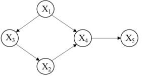
Figure 1. A Bayesian network structure example
The principle behind BNs is the Bayes’ rule, which is used for computing the posterior probability of a target variable as more evidence or information becomes available. The computation of the posterior probability is called belief updating, or evidence propagation. Equation (1) describes the Bayes’ rule.
pxe=p(e|x)p(x)p(e)
(1)
where
xrepresents the value of a target variable (e.g., population change),
erepresents the values of its parent nodes.
pxeis the posterior probability of x given e, p(x) is called prior probability,
pexis the likelihood of e given x, and
p(e)is the probability of e irrespective of the knowledge about
x.
Fitting a BN model includes two steps: BN structure learning and parameter learning. Structure learning determines the optimal or near-optimal graphical model interdependency among variables and suggests a direction of causation (i.e., the directed links). Structure learning in BN is challenging due to the usually large number of variables involved in complex system analysis, and the larger the network size, the more uncertain the knowledge of the variables and the structure describing the relationships. The structure learning process can be based on directly or indirectly implementable knowledge. Directly implementable knowledge refers to expert and stakeholder knowledge. However, relying only on expertise to determine how variables are interrelated is prone to subjective bias and errors (Aitkenhead, 2009). Indirectly implementable knowledge, which derives knowledge from empirical data through learning algorithms, is a second source of knowledge. The learning algorithms is classified into two categories: constraint-based and score-based (Scutari, 201). Score-based algorithms utilize heuristic optimization techniques, where each candidate network is assigned a score reflecting its goodness of fit and then the algorithm will find the network that maximizes the score. Score-based algorithms are generally preferred because they do not rely on very large sample size, as compared with constraint-based algorithms (Koski and Noble, 2012).
In a BN model, a solution of N variables will imply N(N-1) possible links among variables, with a total of
2N(N-1)permutations to consider. When N gets large, it will result in a huge number of permutations which may be impossible to be exhaustively explored due to limited computing resources and the substantial amount of time required. Hill-climbing is a popular score-based approach to find a good BN structure, but it may produce dense and causally incorrect networks (Margaritis, 2000). This study utilizes a genetic algorithm to facilitate the discovery of an optimal BN structure. Genetic algorithm (GA) is a heuristic search and optimization technique inspired by natural evolution. Typically, a GA works through an evolution of a population of candidate solutions to the problem across a number of generations in pursuit of obtaining better solutions (Forrest, 1993; Tsai et al., 2013). Genetic algorithm greatly improves the time needed in the search of an optimal BN model by an ‘evolving’ procedure. This procedure is elaborated in Section 3.4.
Given a network structure, the second step is parameter learning, which is to specify the CPT for each node. The conditional probability is the probability of each node conditioned upon the values of its parent node (where an arrow originates). Counting, expectation-maximization, and gradient descent are three commonly used parameter learning algorithms. The EM algorithm was selected in this study because studies have shown that EM learning is generally more robust than the other two algorithms and it gives good results in a wide variety of situations (Norsys, 2011; Heckerman, 1997).
Compared with other natural-human system modeling approaches, BN has several distinct advantages that make it a powerful tool for representing and modeling complex system dynamics (Schultz and Smith, 2016). First, the natural-human system is represented as a network of nodes and links; the relations among the variables can be visualized easily through the graphical representation of the network (Aitkenhead, 2009). Second, when a hazard occurs or the value of a variable changes, the propagation effects through the entire network can be understood and estimated (Ropero et al., 2014). Third, due to the explicit treatment of uncertainties by means of probability distributions, BNs can represent the complex relationships among variables that are subject to uncertainty. This feature makes BNs especially useful for decision-making purposes (Aguilera, 2011; Frayer et al., 2014; Celio et al., 2014; Li et al., 2010). Finally, BN enables the computation of posterior probabilities given certain evidence. Through the network, we can estimate the effects of changing the value of one variable on the other variables in the form of probability distribution.
In a review study of 1,375 papers on BN listed in ISI web of Knowledge and published in 1990-2010, Aguilera et al. (2011) noted that only 4.2% of the papers are related to environmental modeling. Despite its potential, BNs have rarely been applied in real-world natural-human modeling (Landuyt et al., 2013). A few successful examples are noted here. Celio et al. (2014) modeled land use decisions in a pre-Alpine area in Switzerland by integrating both biophysical data and local actors’ knowledge into a spatially explicit BN. Results from this study show not only which drivers were most important for land use decision-making in the study region, but also how an alteration of these drivers could change future land use. Ropero et al. (2014) used BNs to study the interactions between human and natural subsystems (land use and water flow components). After the model was learned, two endogenous changes (agricultural intensification and the maintenance of traditional cropland) were introduced to the model for scenario simulation. The results show that intensification of the agricultural practices led to a rise in the rate of immigration to the area, as well as greater water losses through evaporation. A landslides susceptibility assessment model in China using BN was developed by Song et al. (2012). A hill-climbing search algorithm was applied to learn the BN structure. The result is a landslide susceptibility map in Beichuan County created on the basis of the posteriori probability calculation. Schultz and Smith (2016) conducted a pilot study in Jamaica Bay to demonstrate how a probabilistic measure of resilience can be assessed for an infrastructure system using a BN. Four functional performance objectives (life safety, housing, utilities, and transportation) were emphasized. The resilience measure is the joint probability of meeting the four objectives with respect to robustness and rapidity of all four system functions. Their results illustrate how practical information can be developed to support decisions about managing coastal systems to meet resilience objectives.
However, limitations exist in Bayesian network modeling. First, the use of discrete variables in BN modeling is a weakness. Most BNs work with discrete variables during model development which causes information loss. When deciding on cut-off values, the discretization method should make the binning sensible and logical (Landuyt, et al., 2013). Second, BN structure learning is a challengeable work, and heuristic search methods to identify the optimal structure are computationally intensive when producing large networks. In spite of these limitations, the successful studies discussed above indicate that BN can be a powerful tool in addressing system complexity (Aguilera et al., 2011; Frayer et al., 2014; Refsgaard et al., 2007).
3. Material and methods
3.1 Study area
Located in southeastern Louisiana, the study area is also known as the Lower Mississippi River Basin (LMRB). The study area covers 26 parishes (i.e. counties), with Lake Pontchartrain serving as an approximate dividing line between the “North” and the “South”. The “South” has been facing a serious land loss problem, which is considered to be a result of both natural and human factors interacting. Dams and levees built to reduce flood risk to the urban area have also reduced the Mississippi River sediments that are necessary to replenish the wetlands. Low elevation, land subsidence, and sea-level rise, together with oil and gas pipelines and canals crisscrossing the wetlands, have contributed to land loss in the “South” over the years (Qiang and Lam 2016; Zou et al., 2016; Twilley et al., 2016). In addition, the region has suffered from recurrent storm surge, flooding, tornado, and hurricanes in a long run. During the last decade, at least five hurricanes (Katrina, Rita, Gustav, Ike, and Isaac) struck this region, and resulted in significant loss of human lives and tremendous property damages (Lam et al., 2009, 2012; LeSage et al., 2011; Qiang and Lam, 2016). All these slow and rapid coastal hazards have contributed in various degrees to population decline in the “South” and population increase in the “North”. From a long-term perspective, these coastal hazards had profound and persistent population impacts on the region. Finding feasible and effective strategies for vulnerability reduction and resilience enhancement in this vulnerable coastal area is a critical challenge. In total, 2,086 block groups were included in this study.
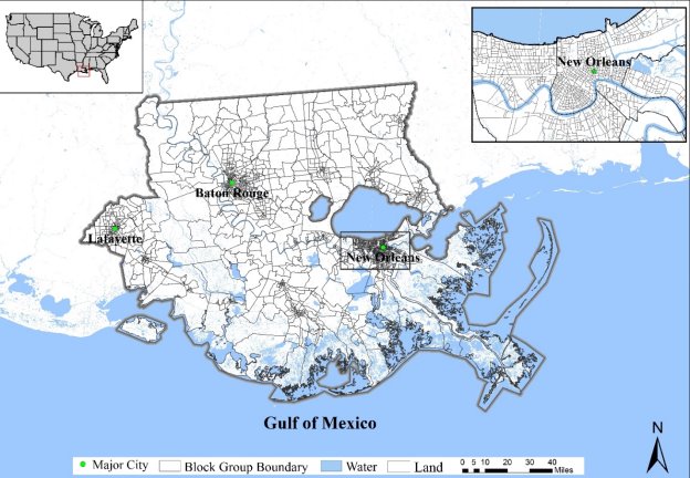
Figure 2. The study area – the Lower Mississippi River Basin
3.2 Data collection and processing
There are a variety of interrelated variables that affect community resilience. There are some commonly recognized variables that have been used to denote different aspects of resilience (Cai et al., 2016; Lam et al., 2016). This paper collected and processed a comprehensive set of resilience variables that were commonly recognized and tested in literature. The data collected were grouped into five dimensions of community resilience: exposure to coastal hazards, property damages incurred, population stability, socioeconomic, and environmental conditions (Figure 3, section a). Property damages, population stability, and socioeconomic variables refer to human subsystem, whereas exposure to coastal and environmental conditions reflect the natural subsystem. The study period was from 2000 to 2010, and the data were collected for this time period whenever available.
3.2.1 Population change, exposure, damages
Population change from 2000 to 2010, indicating the long term outcome of recovery and resilience, was specifically represented as percent of population change. Population stability is a key construct of community resilience, and has been commonly used to indicate the ability of a community to withstand and recover from disasters in disaster resilience literature, especially when the changes happen following disturbances (either increase or decrease) (Elizabeth and Javernick-Will, 2013; Lam et al., 2016). Hence, improving population stability would mean enhancement of community resilience. The percent of population change was calculated by dividing the population difference between 2010 and 2000 by total population in 2000.
There is no public variables on the hazard exposure and damages at the block group level. Therefore, we used the same methodology in Cai et al.(2016) to derive the two variables. Storm surge, hurricane, flood, tornado, tropical storm were the five major types of coastal hazards considered in this study. The Storm Event Database from the National Oceanographic and Atmospheric Administration’s National Climate Center (https://www.ncdc.noaa.gov/) was used to retrieve the chronological listing of the disaster events happened in this study area. The record of each disaster event was at one of the three geographical levels: point, city or county levels. The points were assigned to the block groups they locate in. For city or county level records, spatial interpolation method was used to downscale the city- and county-level data into block groups (Cai et al., 2016; Lam, 1983). Hazard exposure was calculated by the total number of hazard events that occurred in a block group during the ten-year period, adjusted by the weight of the event type and event duration (Cai, et al., 2016; Lam et al., 2016).
The property damage of each block group was the cumulative per capita property damages incurred in the coastal hazards recorded in exposure. The per capita damages of each block group was represented by the cumulative property damages caused by these events from exposure standardized by block group population. The volume-preserving areal interpolation method in Cai et al. (2016) distributes the total value of property damage of a city/county to block group level according to their developed land area. This method is based on the assumption that property damages caused by natural hazards always occur in developed land areas whereas barren land seldom has property damage (Cai et al., 2016).
3.2.2 Socioeconomic and environmental variables
This paper focuses on the preexisting socioeconomic and environmental conditions within communities that affect the disaster impacts and the ability to recover following the disasters. Based on literature review and the availability from public sources, a total of 33 socioeconomic and environmental variables were collected as proxy measures representing different resilience dimensions.
The data was collected from multiple sources. The United States Census Bureau (http://www.census.gov/) provides the census variables in the pre-event year 2000. The National Land Cover Database (http://www.mrlc.gov/) and National Elevation Dataset (http://nationalmap.gov/elevation.html) offers the access to land cover and elevation data. Subsidence rate was obtained and processed by Zou et al. (2016) from the National Geodetic Survey (http://www.ngs.noaa.gov/) using the empirical Bayesian kriging interpolation method. Percent of land loss area was tabulated by the authors using the land area change imagery in coastal Louisiana from the National Wetlands Research Center (http://www.nwrc.usgs.gov/). Flood zone boundary was from National Flood Hazard Layer (http://catalog.data.gov/dataset). The data from multiple sources were all converted to the same geographical scale. Additionally, the raw data were transformed into percent, rates, or averages so that communities of varying sizes and characteristics can be compared. Table 1 lists all the variables prepared for the BN modeling process. Figure 3 shows the entire methodological framework of this study.
Table 1. Population change and 35 natural and human resilience-related variables
| resilience dimension | Resilience concept | Variable | Justification |
| long-term resilience outcome | population stability | % population change 2000-2010 | Lam et al. (2016) |
| exposure | exposure to coastal hazards | hazard exposure | Cai et al. (2016) |
| disaster damage | property damages | per capita damages | Cai et al. (2016) |
| socioeconomic | livelihood stability | % family households | Cassidy and Barnes (2012) |
| wealth/livelihood stability | % owner-occupied housing units | Burton, 2015 | |
| shelter capacity | % vacant housing units | Cutter et al. (2010) | |
| social connection | % 1-person household | Cassidy and Barnes (2012) | |
| age | % population 65 Years and Over | Morrow (2008) | |
| urbanization | % urban population | Cutter et al. (2010) | |
| social isolation | % households with female householder, no husband present | Cutter et al. (2010) | |
| language competency | % households with linguistically isolated | Cutter et al. (2010) | |
| special needs | % population with disability | Cutter et al. (2010) | |
| high education | % over 25 years old with above Bachelor degree | Cutter et al. (2010) | |
| education attainment | % over 25 years old no schooling complete | Cutter et al. (2010) | |
| population density | individuals per square kilometer | Cutter et al. (2010) | |
| transportation access | % housing units with no vehicle available | Cutter et al. (2010) | |
| place attachment | % native-born American population | Cutter et al. (2010) | |
| communication capacity | % housing units with telephone service available | Cutter et al. (2010) | |
| livelihood stability | median household income | Sherrieb et al. (2010 | |
| housing price | median value of owner occupied housing units | Cutter et al. (2014) | |
| poverty | income below poverty level | Cutter et al. (2014) | |
| response capacity | % employment in production, transportation, material moving | NIST (2015) | |
| non-dependence on primary sectors | % not employed in farming, fishing, forestry | Cutter et al. (2014) | |
| employment | labor forces employment rate | Cutter et al. (2010) | |
| housing type | % mobile home units | Cutter et al. (2010) | |
| construction quality | % housing units built before 1970 | Cutter et al. (2010) | |
| potential loss | housing density | Cutter et al. (2010) | |
| school restoration potential | number of schools per 1,000 persons | Few (2007) | |
| response | health care and hospital facilities per 1,000 persons | Cutter et al. (2010) | |
| emergency preparedness | distance to evacuation route | Cutter et al. (2010) | |
| land erosion | % land loss area | Qiang and Lam (2016) |
Table 1 continued
Table 1 continued
| environmental | subsidence | subsidence rate | Zou et al. (2015) |
| land cover | % agriculture land | Burton (2015) | |
| hazard risk | distance to coastline | Qiang and Lam (2016) | |
| hazard risk | % flood zone area | Burton (2015) | |
| hazard risk | mean elevation | Baker (2009) | |
| land erosion | % land loss area | Qiang and Lam (2016) |
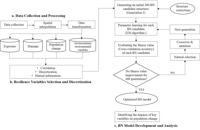
Figure 3. Methods used in this study
3.3 Selecting and discretizing resilience variables
It would be difficult to model population change with all the 35 resilient variables because when the number of variables included in a model is high, the model will become too complex to interpret and cause serious computational challenge (Drees and Liehr, 2015). Also, these variables often exhibit multicollinearity. To make the resulting network representable and reduce the multicollinearity, a hybrid method combining linear correlation analysis and mutual information evaluation was applied to extract only the key, least overlapping variables driving population change (Figure 3b).
First, Pearson’s correlation coefficients among the 35 driving variables were calculated. If the correlation coefficients between any two variables are statistically significant and greater than 0.6, then in the next step, only the variables that have higher mutual information values to population change would be selected for the following modeling.
The second step includes discretizing the resilience variables and calculating their mutual information (MI) with respect to percent of population change. The discretization process is necessary since the ability of BN to treat continuous data is limited. The discretization of these variables should consider both parsimony and the desired representation of the data (Song et al., 2012). To make the discretization logical, in this study, each variable was first standardized into z-score values. Z-score measure how many standard deviations below or above the population mean a raw value is. Each variable was then discretized into six states based on its z-scores. The intervals of the six states, from the minimum to the maximum, corresponding to original values, are [min, µ-2σ), [µ-2 σ, µ- σ), [µ- σ, µ), [µ, µ+ σ), [µ+ σ, µ+2 σ), and [µ+2 σ, max]. µ and σ denote the mean value and standard deviation of a variable. The six states are indexed as states 1, 2, 3, 4, 5, and 6. The discretized variables were further used to calculate the mutual information value between each driving variable and percent of population change.
Mutual information (MI) measures the entropic dependency between two variables. It is the reduction in uncertainty of variable X due to knowing variable Y, and vice-versa (Nicholson and Jitnah, 1998). MI has often been used to decide if the connection between two variables is more significant than others in BN modeling. High value of MI means a large reduction in uncertainty. The variables are independent when mutual information between them is zero. Only the variable with greater mutual information would be selected here. The MI value of a resilience variable X with respect to percent of population change
Yis defined as follows:
IX;Y=∑x∈X∑y∈Ypx,ylog(px,ypxpy) (2)
where
IX;Yrefers to the MI between X and Y, x and y are the distinct values of X and Y,
px,yis the joint probability of X and Y at values x and y, and
pxand
pyare the probabilities of X at x and Y at y, respectively.
Based on the steps above, 10 driving variables, including hazard exposure, per capita damages, population density, percent of households with female householder, percent of owner-occupied house units, employment rate, percent of housing units built before 1970, distance to coastline, percent of flood zone area, percent of agriculture land, were selected for the next BN modeling (Table S1, Supporting information). Table 2 lists the cutoff points of the 11 variables used in the subsequent BN modeling. ‘NA’ means the value within this states is not available for this particular variable.
Table 2. Discretization results of the 11 variables used in BN modeling
| variables | States | |||||
| 1 | 2 | 3 | 4 | 5 | 6 | |
| % population change | [-100,-85.5) | [-85.5, -45.6) | [-45.6, -5.6) | [-5.6, 34.4) | [34.4,74.4) | [74.4, 345) |
| hazard exposure | NA | [1.6,3.2) | [3.2,9.2) | [9.2,15.1) | [15.1,21.1) | [21.1,20.2) |
| per capita damages | NA | NA | [0.6,58617.8) | [58617.8,556618.4) | [556618.4,1054619.0) | [1054619.0, 5505630.8) |
| population density | NA | NA | [0, 171.3) | [171.3, 364.0) | [364.0,556.6) | [556.6, 2171.1) |
| % households with female householder | NA | [0, 5.3) | [5.3, 18.1) | [18.1, 30.8) | [30.8,43.6) | [43.6, 100) |
| % owner-occupied house units | [0,13.6) | [13.6,37.0) | [37.0,60.5) | [60.5,84) | [84, 100) | NA |
| employment rate | [0, 75.4) | [75.4, 83.6) | [83.6,91.7) | [91.7, 99.8) | [99.8,100) | NA |
| % housing units built before 1970 | NA | [0, 22.0) | [22.0, 51.9) | [51.9, 81.8) | [81.8, 100) | NA |
| distance to coastline | NA | [0.12, 2.0) | [2.00, 22.9) | [22.9, 43.9) | [43.9, 64.8) | [64.8, 103.0) |
| % flood zone area | NA | [0,14.0) | [14.0, 51.2) | [51.2, 88.5) | [88.5, 100) | NA |
| % agriculture land | NA | NA | [0, 9.8) | [9.8, 28.5) | [28.5, 47.3) | [47.3, 90.0) |
3.4 Developing an optimized Bayesian network model
To implement the genetic algorithm, the structure of a candidate Bayesian network was represented as a binary string that crossover and mutation operations could be applied to in subsequent steps (Larrañaga et al., 2013). Each binary string is considered as a chromosome (Figure S1, Supporting information). In the binary string, 1 denotes the presence of a link between two variables and 0 denotes the absence of link. For the 11 variables (the output variable percent of population change and the 10 resilience variables) considered in this study, each variable has 10 possible links to the other variables. Therefore, every binary string consists of 11×10=110 bits. Each bit in the 110-digit binary string corresponds to one of the links between variables in the order as following: X1to X2, X1 to X3, …, X1to X11, X2to X1, X2to X3, …, X11to X9, X11to X10.
To start the evolution process, the first step is to randomly initialize a population of 200 chromosomes as the first generation. Each chromosome defines a candidate structure of Bayesian network. Given the structures, the parameters (conditional probability table (CPT)) at each node for each candidate network were learnt from the empirical data. The expectation-maximization (EM) algorithm, discussed in Section 2, was used to learn the BN parameters.
After parameter learning for all the candidate BNs in one generation, the goodness-of-fit of each candidate BN was then evaluated through a fitness value (Aitkenhead, 2009). In this case, the goodness-of-fit of a chromosome means the robustness and inferential ability of a BN model. This study used the 10-fold cross-validation accuracy as the fitness value to evaluate the model performance. The cross-validation approach aims to check how predictive a model is when confronted with data that have not been used previously for learning the model, thus enabling model validation. For this study, the dataset was divided into 10 subsets. For each iteration, the BN model was trained using 9 subsets and the trained model was used to validate the population change classification of the remaining subset. By repeating the cross-validation 10 rounds, each subset was tested once. The resulting 10 prediction accuracies were then averaged as the cross-validation accuracy (Refaeilzadeh et al., 2009). Compared with the single classification accuracy method, the cross-validation approach avoids model overfitting and improves the predictive power of Bayesian Networks.
In each generation, the fitness values of all 200 chromosomes were calculated and then ranked from the highest to the lowest. Natural selection process was implemented to choose the most fitted models to survive and reproduce. In this study, the 10 most fitted networks in each generation would survive as parents and bred with each other to reproduce a total of 200 offspring solutions as the next generation population, and the process continued until no improvement in fitness values for 400 generations is reached.
Certain restrictions derived from domain knowledge were applied to the network structure to save search time with illogical and unreasonable Bayesian network. The output node of the network is percent of population change herein, and other selected resilience variables are the input nodes of the network. Thus, the BN should have at least one link from these input variables to population change because population change is impacted by other variables, and no link from population change to the input variables because the input variables are caused or impacted by among themselves. Furthermore, each input variable should have at least one link, either directly or indirectly, to the target variable population change. At the beginning of each generation, every candidate structure was checked to examine these restrictions. The candidate structure that did not conform to these restrictions would be excluded in order to avoid wasting search time.
The reproduction operators involve mutation and crossover (Figure S1, Supporting information). Crossover means the swapping of portions of the chromosomes of a pair of parents to generate offspring reflecting good features of their parents or even surpassing them (Forrest, 1993). Mutation, which follows the crossover process, is performed on individuals in the child population by randomly changing a bit of the chromosome (i.e., randomly changing the presence of connections to absence). Mutation aims to increase population diversity and prevent GA falling into local extremes, but it should not occur very often to avoid reducing GA into random search. In this study, the probability of crossover was specified as 0.8 which means every 8 out of 10 children were produced through crossover operation. The mutation probability was set to 0.1, meaning 1 out of 10 bits on a chromosome (on average) picked at random will be altered.
With the application of these operations, the next generation was derived, whose individuals were then evaluated and ranked based on their fitness values (Aitkenhead, 2009). The evolution repeated until it meets the stopping criterion that no improvement of fitness values for 400 generations. Finally, the top ranked individual was reported. Figure 3.c demonstrates how this optimization procedure was carried out.
3.5 Identifying the impacts of key variables on population change
After the optimal BN model was constructed, the relationships between population change and its influencing resilience variables were further identified by taking the advantage of the belief updating capability of BN (Frayer et al., 2014). By assigning a specific state to one or more nodes, the ‘evidence’ is entered into the network. Belief updating, a form of probabilistic inference, calculates the posterior probabilities for the states of other nodes in the BN (Norsys, 2011). This study focuses on how an individual driving variable could affect population change. Therefore, suppose each time only one node is assigned by a specific state, and the other nodes are not observed, the posterior probability of population change could be obtained with a belief updating algorithm. By repeating this process, the posterior probability of population change conditioned on every state of the other nodes were obtained. The junction tree (JT) is one of the most popular belief updating algorithm and was applied to calculate the posterior probability of the target node. (Song et al., 2012).
The genetic algorithm for optimizing the BN structure was programed by the first author and carried out using R. After the final BN structure was confirmed, the impacts of resilience variables on population change was analyzed using the Bayesian network development software Netica (Norsys, 2011).
4. Results and discussion
4.1 Optimized Bayesian network model
Figure 4 shows the median, mean and maximum fitness values of every generation in the genetic algorithm. Over a period of 906 generations, the fitness values (cross-validation accuracies) increased rapidly at first, then slowed down and finally converged upon the optimal value. The genetic algorithm yielded an optimized Bayesian network structure with a cross-validation accuracy of 67%. Once the optimal network structure was yielded, the BN model parameters were trained with the complete dataset using an EM algorithm. The final BN model contains two main components: a network structure of 11 nodes and a Conditional Probability Table (CPT) of each node.
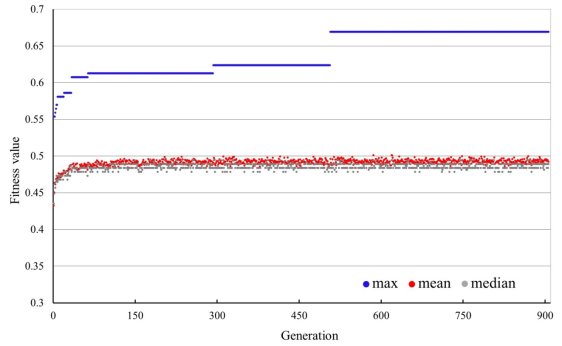
Figure 4. Changing fitness values with generations
Figure 5 shows the optimized BN, where six variables (hazard exposure, per capita damages, distance to coastline, employment rate, percent housing units built before 1970, and percent households with female householder) were found to be the direct drivers of percent population change. Of the six direct variables, hazard exposure also had direct impact on per capita damages, which in turn affected population change. The variable employment rate was influenced by multiple variables, including percent flood zone area, percent owner-occupied housing units, population density, and percent housing units built before 1970. On the contrary, distance to coast and percent female householder, the other two variables directly impacting population changes, did not link to any other variables. The remaining four variables (percent agriculture land, percent flood zone area, percent owner-occupied housing units, and population density) had indirect links to percent population change. Percent agriculture land influenced population change indirectly through percent flood zone area and employment rate.
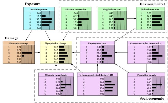
Figure 5. The optimized BN with hazard exposure (node in blue), per capita damage (node in orange), environmental (nodes in green) and socioeconomic variables (nodes in purple) interacting and influencing population change (node in yellow)
Figure 5 also shows the a priori probability distribution of each variable. The a priori probability distribution is the initial probability distribution of a variable irrespective of any other variable. For instance, Figure 5 indicates that 48.4% of the block groups had percent population change below its mean value (-5.6%) (states 1-3 combined), or 27.5% of all the block groups fell into state 5 which means over 88.5% of their land lying within flood zone.
The conditional probability table (CPT) of each node is the quantitative component of a BN. Each cell of the CPT is a conditional probability for the node being in a specific state, given a specific configuration of its parents’ states (Song et al., 2012). Thus, the number of cells in a CPT equals the product of the number of possible states for this node and the numbers of all possible states for its parent nodes. For example, as shown in Figure 5, percent population change has 6 possible states and has six parent nodes. The CPT of percent population change is a table of 66 cells (Table S2, Supporting information).
4.2 Impacts of socioeconomic and environmental variables
As discussed in Section 3.5, this study further investigate how each variable influenced population change through belief updating, by assuming the probability of a specific state of one node is 100% every time iteratively. The states that are not available for a variable were not considered in this part due to their low chance of happening in reality. We used the total probability of the three population change states (states 1, 2, 3), corresponding to the real value -100% to -5.59%, to indicate the probability of population decrease (-5.59% is the mean of percent of population change in the region). Figure 6 shows the probability of population decrease versus the six direct variables, with the black solid lines tracing the probability value of population decrease at each state of the six variables and the red dash lines being the linear trend lines fitted through the known points for ease of comparison.
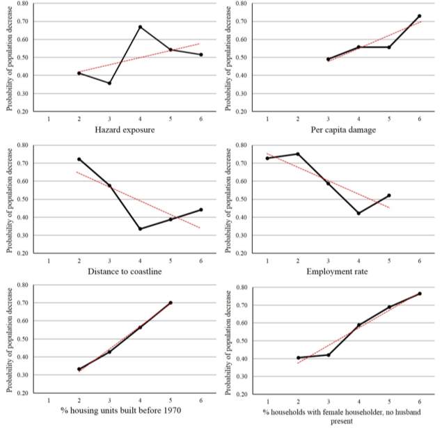
Figure 6. Probability distribution of population decrease versus the six direct resilience variables
Based on Figure 6, hazard exposure has a nonlinear influence on population decrease, with population decrease probability fluctuating along the exposure axis. The overall trend, however, is upward, indicating higher exposure generally leading to more population loss. Similarly, population tends to decrease with increasing per capita damages from coastal disasters. The population decrease probability is as high as 0.73 when the damage is at the highest level. This result suggests that higher hazard exposure does not necessarily drive people out, but people would be more likely to leave if more damages are incurred from these events.
The population decrease probability decreases with increasing distance to coastline, though the response is not linear. In general, the results suggest that the closer the distance of a community to the coastline, the more probable the community will lose population. The highest population decrease probability (0.72) occurs when the distance to coastline is as short as between 0.12 and 1.98 kilometers. When a community is closer to the coastline, it means that the community is usually under a much higher risk of being affected by coastal disasters and faces more pressure for disaster recovery.
Regarding the socioeconomic component, employment rate has a large influence on population decrease, but the response is also not linear. In general, the higher the employment rate, the lower the probability of population decrease. Communities having over 92% (state 4) of their labor forces being employed would only have a 0.42 probability of population loss, compared with a 0.75 probability of population decrease when the employment rate is less than 84% (state 2). This is expected as communities with higher employment rates generally have the resources and abilities to adapt and return after a disruption.
Population decrease becomes more likely as percent housing units built before 1970 increases. The relationship is nearly linear, in other words, the higher the percent of housing units built before 1970, the higher the probability of population decrease. As late as 1950, one third of the housing units in the U.S. lacked indoor plumbing, full kitchen facilities, or both. It is by 1970 most housing had these features and the housing quality had a continuous improvement that enhanced the capacity to withstand disturbances (Lopez, 2012). Therefore, percent housing units built before 1970 reflects the overall construction quality of housing and also the level of development of the community.
The variable percent female householder is considered an indicator of poverty from the literature, which was found to have a direct, positive, and close-to-linear relationship with the probability of population decrease in this study. The probability of population decrease rises to 0.76 when percent of female householder is over 44% (state 6). From the correlation analysis in Section 3.3, the variable poverty rate had a significant positive correlation with this variable (r = 0.56). Percent female householder is also an important indicator used in the Berkman-Syme Social Network Index to measure social isolation (Cassidy and Barnes, 2012; Martin, 2015). Due to limited support for dependent care and lack of social connections, female householders have to struggle with both job responsibilities and care for family dependents, which would make them less likely to have resources to get better prepared for and recovered from disasters.
The above analysis indicate that every individual variable plays its own role, either linear or nonlinear, in shaping the population change pattern in a region subject to frequent coastal hazards. A single variable may only has limited extent to alter the posterior probability distribution of population change, but the changes of multiple variables would amplify the effects on the recovery outcome significantly as a whole. A more detailed scenario analysis will be conducted in future studies.
Several limitations of this study are noted here. First, although the cross-validation accuracy shows that the derived model is feasible and robust, the BN derived depends highly on the variable selection, discretization, and model construction methods. Sensitivity analysis could be considered in future research to understand how these various steps would affect the final model. Second, the results derived is subject to context, scale, and region. This method could be tested at different spatiotemporal scales, in different regions, to derive reliable insights on how the resilience process varies with changing scales and regions. Third, the final BN model is useful for modeling the complex and multi-faceted resilience process, but feedback loops, an inherent component of complex systems, were not modeled in this study. A dynamic Bayesian network can be considered in future research to overcome this limitation by repeating the network structure at two (or more) time-steps and adding links between time-steps.
5. Conclusion
The primary motivation of this research was to uncover a set of important resilience variables that could account for the spatial variation of population changes in a region vulnerable to coastal hazards. Specifically, the focus of the paper was to identify and quantify the interactions among these driving variables in a probabilistic form, the results of which can then be used for future scenario modeling and planning for resilience. An optimal Bayesian network model was developed to explain the population change dynamics using data at block group scale. The study first extracted 10 variables from a group of 35 to derive the network. Through a genetic algorithm and after 906 generations, the resultant optimized Bayesian network was achieved with a cross-validation accuracy of 67%. The expectation-maximization (EM) method was used to learn the conditional probability tables, and the junction tree (JT) algorithm was applied to compute the posterior probabilities. Six variables were found to have direct impacts on population change, including hazard exposure, hazard damages, distance to coastline, employment rate, percent housing units built before 1970, and percent households with female householder. The remaining four variables are indirect variables, including percent agriculture land, percent flood zone area, percent owner-occupied housing units, and population density. Each variable has a conditional probability table so that its impacts on the probability of population change can be evaluated as it propagates through the network. These probabilities could be used for scenario modeling in future studies to help inform policies to reduce vulnerability and enhance resilience.
While future improvements of the study will need to be made, this paper contributes to the literature in three major aspects. First, the paper contributes to the few empirically based approach that aims to investigate the dynamics of community resilience by taking both natural and human components into consideration. Literature on modelling the dynamics of a complex natural-human system in the context of community resilience to hazards is rare. This study increases our knowledge of how natural disasters and community capacity impact population changes and ultimately disaster recovery. Second, in terms of methodology, this paper contributes by demonstrating the procedures needed to couple Bayesian network with genetic algorithm, which has been proven to be effective in deriving an optimized BN. The uncertainties that result from the high complexity of the systems are explicitly handled in the form of probability distribution. Lastly, the final BN model can be used to simulate potential spatial patterns of population change. When an “evidence” is introduced into the network, the systematic changes of all the nodes involved in the network could be modeled. The simulation ability will be useful for decision-makers to evaluate potential effects of certain scenarios and help develop actionable adaptation strategies.
Acknowledgements
This work was supported by two research grants from the U.S. National Science Foundation: one under the Dynamics of Coupled Natural Human Systems (CNH) Program (award no: 121211), and the other under the Coastal Science, Engineering and Education for Sustainability (Coastal SEES) Program (award no: 1427389). Support by a NOAA-Louisiana Sea Grant (Grant No. R/S-05-PD) is also acknowledged. Any opinions, findings, and conclusions expressed in this paper are those of the authors and do not necessarily reflect the views of the funding agencies.
Supporting information
Table S1. 10 selected driving variables and their mutual information values to percent of population change
| selected variables | resilience dimension | mutual information |
| hazard exposure | exposure | 323.9 |
| per capita damage | disaster damage | 177.3 |
| population density | socioeconomic | 271.6 |
| % households with female householder, no husband present | socioeconomic | 232.3 |
| % owner-occupied house units | socioeconomic | 198.4 |
| employment rate | socioeconomic | 196.1 |
| % housing units built before 1970 | socioeconomic | 258.2 |
| distance to coastline | environmental | 230.0 |
| % flood zone area | environmental | 201.9 |
| % agriculture land | environmental | 155.4 |
Table S2. Part of Conditional Probability Table (CPT) for the node
percent of population change
| employment rate | Percent of population change | |||||
| 1 | 2 | 3 | 4 | 5 | 6 | |
| 1 | 0.167 | 0.167 | 0.167 | 0.167 | 0.167 | 0.167 |
| 2 | 0.143 | 0.143 | 0.286 | 0.143 | 0.143 | 0.143 |
| 3 | 0.056 | 0.056 | 0.278 | 0.167 | 0.333 | 0.111 |
| 4 | 0.023 | 0.023 | 0.295 | 0.091 | 0.500 | 0.068 |
| 5 | 0.125 | 0.125 | 0.125 | 0.125 | 0.375 | 0.125 |
| 6 | 0.167 | 0.167 | 0.167 | 0.167 | 0.167 | 0.167 |
Table S2 demonstrates a portion of the CPT of percent population change relative to employment rate when all the other 5 parent nodes conditioned on state 3. For instance, under the condition that employment rate is at state 4 (91.7% to 99.8%), and all other variables at state 3, population change has the highest probability (0.5) to be at state 5 (34.4% to 74.4%).
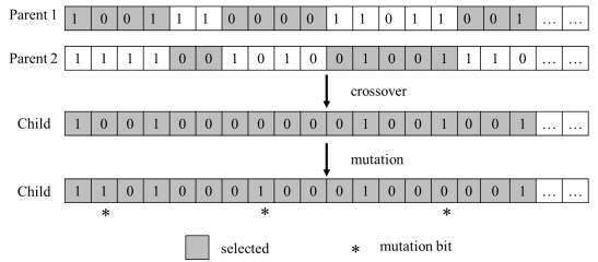
Figure S1. Reproduction operators (crossover and mutation)
Cite This Work
To export a reference to this article please select a referencing stye below:
Related Services
View all


Related Content
All TagsContent relating to: "Geography"
Geography is a field of study that is focused on exploring different places and environments from around the world. Different aspects of Geography include countries, habitats, distribution of populations, the Earth's atmosphere, the environment, and more.
Related Articles

DMCA / Removal Request
If you are the original writer of this dissertation and no longer wish to have your work published on the UKDiss.com website then please: