Reliability-based Design of Rainwater Harvesting Systems
Info: 17258 words (69 pages) Dissertation
Published: 15th Nov 2021
Tagged: Environmental StudiesTechnology
An Investigation into the Reliability-based Design of Rainwater Harvesting Systems in the UK under Current and Future Climatic Conditions
Abstract
This dissertation investigates the relationship between key rainwater harvesting (RWH) variables and the resulting system reliability these provide, before exploring how this relation might be affected by climate change. As such, graphs specific to various UK regions are produced, linking the local precipitation (rainfall) regime, domestic water demand, catchment area, storage capacity and system reliability for both the present-day and 2080 forecasted climate. For the purposes of demonstration, the study focuses on two UK regions: North Scotland (NS), and South West England and Wales (SWEaW).
The use of rainwater harvesting systems (RWHS) in the UK was chosen as a field of study since although numerous studies have proved their effectiveness in various geographical contexts, the UK has failed to embrace this practice on a wide scale. More importantly, current UK guidelines do not consider reliability as a design parameter and ignore the potential impact of climate change on system performance. Consequently, when sizing their storage tanks as per UK guidelines, residents wishing to install RWHS do not know what reliability the recommended storage size will provide today or in the future.
To produce the reliability graphs artificial monthly rainfall series produced by a stochastic (random but statistically describable by a probability distribution) rainfall generator were used to simulate RWHS behaviour and thereby calculate reliability. This process was repeated for many possible parameter combinations and results were plotted. To model future reliability, the artificial rainfall series were modified to reflect predicted changes in rainfall as a result of climate change. These modified precipitation series were then once again used in simulations to obtain revised reliability values. Thereafter, differences in various reliability definitions and rainfall series types were compared and analysed to determine which produced the most accurate and meaningful results. Finally, a case study was presented to demonstrate how the graphs produced could be used for reliability assessment or reliability based design.
Results showed that the use of artificially generated monthly rainfall series accurately simulated reliability on a monthly basis, but that the use of daily simulation intervals could further improve simulation accuracy. The wide range in predicted changes in rainfall meant that simulated future reliabilities were also marked by a high degree of uncertainty. However, based on central climate change estimates, reliability was expected to decrease in most cases. Nevertheless, the graphs proved that RWHS can be highly effective.
These graphs could be used for two purposes: assessment or design. For the former, the graphs could be incorporated into the UK guidelines to allow designers to determine the reliability achieved by the recommended storage capacity. Their second purpose could be for designer to identify possible parameter combinations required to achieve a desired level of present-day or future reliability. In an attempt to try promote RWHS in the UK, it is hoped that these graphs will facilitate their design and emphasize their potential effectiveness.
Click to expand Table of Contents
Table of Contents
1 List of Figures
2 List of Tables
3 Introduction
3.1 RWHS and their History
3.2 Sizing of Rainwater Harvesting Storage Tanks
3.3 Objectives and Scope
3.4 Overview of Dissertation Structure
4 Literature Review
4.1 Significance of Domestic RWHS
4.1.1 Growing Importance and Benefits
4.1.2 Previous Studies showing Impact
4.2 Studies on the Sizing of RWHS
4.2.1 Scope, Purpose and Output
4.2.2 Parameters Considered
4.2.3 Assessment of Performance
4.2.4 Methodology
4.2.5 Rainfall Series
4.3 Stochastic rainfall generators
4.3.1 Overview
4.3.2 Method of Fragments
4.4 RWH in the UK:
4.4.1 Importance & Use
4.4.2 UK Sizing Guidelines
4.4.3 UK RWH Parameters
4.5 Climate Change Impact on Precipitation
5 Methodology
5.1 Overview and Rationale of Approach
5.2 Defining the Hydrological Year
5.3 Fitting Probability Density Functions to Annual Rainfalls
5.4 Generating Monthly Rainfall Series
5.5 Calculating Current Reliability
5.6 Incorporating Effects of Climate Change
6 Discussion and Analysis of Results
6.1 Accuracy of Stochastic Rainfall Series
6.1.1 Accuracy of Annual Stochastic Rainfall Series
6.1.2 Accuracy of Monthly Stochastic Rainfall Series
6.2 Method of Fragments: Impact of Subset Size
6.3 Assessment of Reliability
6.3.1 Comparison of Volumetric and Temporal Reliability
6.3.2 Comparison of Monthly and Daily Reliability
6.3.3 Comparison of Historic and Generated Reliability
6.4 Reliability in 2080
6.4.1 Dry Scenario
6.4.2 Wet Scenario
6.4.3 Median Scenario
7 Case Study
7.1 Overview
7.2 Simplified Approach
7.3 Intermediate Approach
7.4 Corresponding Reliabilities and Discussion
8 Conclusion
8.1 Further Work
8.2 Closing Comments
9 Bibliography
Click to expand list of figures and tables
1 List of Figures
Figure 1: Dimensionless Design Curves (Fewkes, 1999)
Figure 2: Storage Sizing Contour Map (Liaw & Tsai, 2004)
Figure 3: Simplistic Approach to sizing RWHS (Gould 1999)
Figure 4: UK weather regions (Legg, 2017)
Figure 5: UK precipitation change predictions (Defra, 2009)
Figure 6: Methodology flowchart
Figure 7: Bar chart of correlation values between consecutive monthly rainfall values for NS
Figure 9: Annual precipitation histogram and fitted Normal probability density function for NS
Figure 9: Mass balance algorithm flowchart
Figure 11: Percentage change in monthly precipitation for 2080 dry, median and wet projections in SWEaW
Figure 12: Mean monthly precipitation values for current and future stochastic rainfall series in SWEaW
Figure 13: Empirical and theoretical cumulative probability functions for annual rainfall in SWEaW.
Figure 14: Sample and theoretical quantiles of annual rainfall in SWEaW
Figure 15: Boxplot of generated and historical monthly precipitation for SWEaW
Figure 16: Scatter plot of monthly rainfall for historical and generated rainfall series (using 5% of sets of fragments) in NS.
Figure 17: Scatter plot of monthly rainfall for historical and generated rainfall series (using 100% of sets of fragments) in NS.
Figure 18: Violin plot of monthly rainfall for historical and generated rainfall series (using 5% of sets of fragments) in NS.
Figure 19: Violin plot of monthly rainfall for historical and generated rainfall series (using 100% of sets of fragments) in NS.
Figure 20: Volumetric and temporal reliabilities using generated monthly rainfall series for SWEaW
Figure 21: Daily and monthly reliabilities using historic rainfall series for SWEaW
Figure 22: Generated and historic monthly reliabilities for SWEaW
Figure 23: Enlargement of Figure 4.3.3-1
Figure 24: Current and future dry-scenario reliabilities for SWEaW
Figure 25: Current and future wet-scenario reliabilities for SWEaW
Figure 26: Current and future median-scenario reliabilities for SWEaW
Figure 27: Current and future median-scenario reliabilities for NS
Figure 26: Annual average rainfall depths across the UK (BS 8515)
Figure 29: Simplified approach storage sizing graph for 4-person household (BS 8515)
Figure 30: Enlargement of graph depicting current and future monthly reliabilities for SWEaW
Figure 31: Enlargement of graph depicting current monthly reliabilities for SWEaW
2 List of Tables
Table 1: Percentage changes in winter and summer rainfall for dry, median and wet scenario in SWEaW and NS
Table 2: Distribution goodness-of-fit tests to model annual rainfall in SWEaW
Table 3: Recommended storage capacities as per intermediate approach (BS 8515)
3 Introduction
3.1 RWHS and their History
Rainwater harvesting (RWH) is a process comprising the collection, distribution and use of rainwater (Basinger, et al., 2010). The collection can occur via any catchment area, such as a field on a large scale, or a roof on a domestic scale. Due to the non-uniform distribution of rainfall over time, tanks are usually installed so that rainwater may be stored and used when needed (Su, et al., 2009). The nature of the storage system also depends on its scale: dams are on the larger end of the spectrum, storing water for entire communities, whereas domestic storage tanks lie on the smaller end of the spectrum, storing water for only a few individuals or families. The use of the water varies across agricultural, industrial or residential sectors (Hanson & Vogel, 2014). On a domestic scale, rainwater harvesting systems (RWHS) may be used as a primary water source, but in developed countries they are mostly employed as a supplementary water supply for non-potable purposes such as toilet flushing, clothes washing or outdoor watering (Environment Agency, 2010).
An ancient practice, RWH has been employed for thousands of years by many civilisations, such as the ancient Greeks, Romans and Etruscans, for a variety of purposes (Boers & Asher, 1982). Its first application dates to 2000BC when it was used for agricultural irrigation in Jordan (Hanson & Vogel, 2014). During the Middle Ages, RWH was used in Venice as a means of providing domestic water supply (Basinger, et al., 2010). Hanson and Vogel (2014) argue that its popularity as a supplementary water source in urban and suburban areas has increased over the past decades, both in developing and developed countries. Unfortunately, when compared to other developed countries, the UK has failed to embrace and promote RWHS on a large scale (Berndtsson, 2004). Fewkes (2012) suggests this issue may become especially significant given the increasing stress on the UK’s centralised water supply infrastructures, especially in highly populated regions where water is already deemed to be scarce.
3.2 Sizing of Rainwater Harvesting Storage Tanks
The reliability of a RWHS is determined by the relationship between the inflow of water into the storage tank (dependent on the local precipitation regime and catchment area), the outflow of water from the storage tank (dependent on the demand), and the storage capacity, which limits the quantity of water that may be stored at any point in time (Basinger, et al., 2010). Thus, as Hanson and Vogel (2014) argue, “the most important and difficult design decision is how much storage capacity to build”, since this is usually the only parameter controlled by the designer, and often the most expensive part of the RWHS (Lee, et al., 2000). Furthermore, Imtaez et al. (2011) argue that the lack of information on optimal storage size, and on effectiveness of RWHS, are the key factors hindering the widespread use of RWHS.
Current UK guidelines for the design of RWHS are outlined in the 2009 British Standard 8515: Rainwater harvesting systems – Code of practice (BS). The BS proposes three methods for sizing tanks, of which only two are thoroughly explained. However, these two methods consider neither the seasonal variation of rainfall nor the reliability that certain storage sizes will provide. Thus, a house owner wishing to install a RWHS will not know with what reliability a given storage tank will meet his domestic non-potable water demand.
The BS also ignores the impact of climate change. Studies agree that the UK precipitation regime will develop greater variance: summers will become drier and winters will become wetter (Defra, 2009). Since the BSfails to address reliability in the first place the omission of this phenomenon is less evident. However, for a reliability-based storage sizing approach it seems intuitive that the change in one of the key parameters – the precipitation regime – should be considered.
3.3 Objectives and Scope
The first aim will be to produce regional graphs, relating the local precipitation regime, catchment area, daily demand, storage capacity and reliability. Two UK regions with differing rainfall regimes – Northern Scotland (NS) and South West England and Wales (SWEaW) – will be selected for the purposes of demonstration. Precipitation data for SWEaW and NS start in 1873 and 1931 respectively. To choose representative UK parameter values the scope of the study will be defined as follows. First, the study will be limited to the use of RWH for non-potable domestic purposes. As such, only demand for toilet flushing and clothes washing will be considered. Second, it will be assumed that rainfall will be collected via the roof area. Lastly, storage sizes similar to those available on the UK market will be considered.
The second objective will be to explore how the reliability of RWHS might change as a result of climate change. This will involve using the 2009 UK Climate Change Projections (Defra, 2009)to assess how rainfall might evolve under dry, median and wet future scenarios.
Finally, a case study will be presented. Two UK cities will be chosen, RWH storage sizes will be determined using BS guidelines, and the reliability graphs produced will be used to determine the reliability of the RWHS under present-day and future climate conditions. Furthermore, it will be demonstrated how the graphs may be used to identify parameter combinations to achieve a desired level or reliability.
3.4 Overview of Dissertation Structure
The dissertation is structured in the following manner. A literature review will first be undertaken, which will discuss the significance of RWHS, storage sizing methods, artificial rainfall generation and the impact of climate change on UK rainfall. Thereafter the methodology, which was used to generate synthetic rainfall, simulate RWHS behaviour, create the reliability plots, and modify these to account for climate change, will be presented. These results will then be analysed and discussed. The case study, mentioned above, will then ensue. Finally, the conclusion, recommendations for further study and final remarks will be shared.
4 Literature Review
4.1 Significance of Domestic RWHS
4.1.1 Growing Importance and Benefits
The increased global water demand (Fewkes, 2012) and effects of climate change have put water supply infrastructures around the world under stress (Imtaez, et al., 2011). This is especially evident in the many cities that have experienced large urban growth throughout the 20th century (Imtaez, et al., 2011).
To face the problem of increasing water scarcity, Postel (1992) argues that the most direct source of fresh water – rain – should not be ignored. RWHS can provide a sustainable alternative water supply (Basinger, et al., 2010), especially in cities, where the large impervious roof areas make them a viable option (Liaw & Tsai, 2004).
In developed regions, RWHS are primarily used as a secondary water supply for non-potable domestic uses (Su, et al., 2009). Nevertheless, they can help reduce stresses on urban water infrastructures (UWIs), by reducing urban potable water demand and storm water discharge. Thus, they help increase resilience of UWIs to drought, population growth, and floods (Basinger, et al., 2010). Furthermore, if engineered correctly, RWHS can have cost benefits and reduce energy consumption, making them an integral part of “green building” design (Guo & Baetz, 2007).
In less-developed or developing countries, RWHS can be even more important as they are often used as a major / primary water supply (Su, et al., 2009), due to their ability to improve household water access without government infrastructure support or economic aid. Furthermore, RWHS may have numerous advantages over centralised water treatment systems, such as increased reliability, simplicity, and lower cost (Cowden, et al., 2008).
4.1.2 Previous Studies showing Impact
Previous studies, conducted in various regions around the world, have concluded that RWH could considerably reduce the water currently having to be supplied by centralised water infrastructures.
Ghisi et al. (2007) estimated that in Brazil, a rapidly developing country, RWHS could reduce residential potable water demand by as much as 48% in the south east of the country, and 100% in the north. In the developed world, the impact of RWHS can be just as significant: studies have deemed that in Germany, the use of RWHS for toilet flushing could reduce domestic water demand by 30-60% (Hermann & Schmida, 2000).
In Jordan and in Australia – arid regions where the problem of water scarcity is even more pronounced – estimates have concluded that RWHS could reduce potable water demand by up to 20% (Abdulla & Al-Shareef, 2009) and 60% (Coombes, et al., 2000) respectively.
Zhang et al. (2009) demonstrated that in megacities like Beijing, the use of RWHS for water flushing could reduce potable water demand by 25%. Even in NYC, one of the world’s most densely populated cities, studies have estimated that RWHS could meet up to 40% of the toilet flushing water demand (Basinger, et al., 2010).
4.2 Studies on the Sizing of RWHS
4.2.1 Scope, Purpose and Output
Many studies have been undertaken on RWHS, each varying in scope, purpose and output.
Since a key parameter influencing the performance of RWHS is the local weather regime (discussed in section 4.2.2), all studies are confined to a geographical area. Some aim to focus on particular cities, such as Taipei (Su, et al., 2009), NYC (Basinger, et al., 2010), Melbourne (Khastagir & Jayasuriya, 2010) or Nottingham (Fewkes, 1999), whilst other try to generalise across entire countries or regions such as Taiwan (Liaw & Tsai, 2004), USA (Hanson & Vogel, 2014) or Sub-Saharan West Africa (Cowden, et al., 2008).
Most of these studies focus on the use of RWHS for domestic purposes, but some consider their use in agriculture. Lee et al. (2000), for instance, investigated the use of RWHS for tea cultivation. Nevertheless, the aim for most RWHS studies is to provide a method enabling domestic users to size their system for desired levels of reliability.
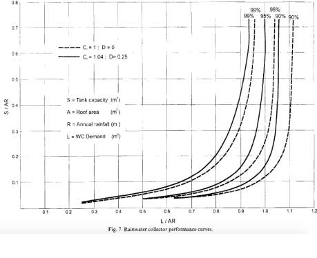
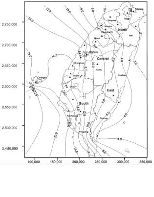
The output of RWHS investigations usually fall into three categories: curves, contour maps, or equations. The first category includes graphs that try to establish the relationship between the various parameters considered. One example would be the dimensionless curves produced by Fewkes (1999), shown in Figure 1, relating catchment area, demand, rainfall level, system efficiency and storage volume. The second category comprises maps with contours showing the required storage capacity to achieve a given reliability. Figure 2 is an example of a map with contours indicating the required storage capacity (in m3) for a volumetric reliability of 90%, a roof area of 100m2and a daily dwelling water demand of 150l (Liaw & Tsai, 2004). Although such maps are easy to understand and quick to read, the infinite number of parameter combinations and many graphs that would therefore need to be published make them impractical. The third category constitutes empirical regression formulae and analytically derived equations defining the relationship between various parameters. Equations (1) and (2) are examples of such formulae, the former being derived analytically (Guo & Baetz, 2007), and the latter being derived via linear regression methods (Hanson & Vogel, 2014).
| Re=AϕψAϕψ+ζGe-ζvff1-e-ζBAϕ-ψBG |
(1) |
| Sr=eaeb1-lnαdμwc11+ρ1-ρc2 | (2) |
Since the aim of such equations is to help users determine the storage size, their complexity and non-user-friendly appearance are of clear disadvantage. Furthermore, since such equations often attempt to generalise parameters across wider geographical regions their accuracy may sometimes be poor. For instance, when testing the regression curves they developed for Greater Melbourne using mass balance simulation methods (discussed in section 4.2.4), Khastagir and Jayasuriya (2009) found that both methods gave recommended storage capacities that differed by up to 30%.
4.2.2 Parameters Considered
Parameters used in the design and performance of RWHS largely remain the same (Hanson & Vogel, 2014) and can be divided into three categories: those affecting the water supply, the water demand, or the financial viability. Most studies choose an array of possible parameter values (Imtaez, et al., 2011 ; Khastagir & Jayasuriya, 2010 ; Rahman, et al., 2012) and assess how different combinations of these impact system performance. To reduce the number of parameter combinations, some studies use average parameter values (Basinger, et al., 2010 ; Su, et al., 2009 ; Cowden, et al., 2008 ; Liaw & Tsai, 2004), whilst others (Fewkes, 1999) assemble several parameters into dimensionless coefficients.
Four factors determine the supply of water: the local precipitation regime, the catchment area, the storage capacity and the runoff coefficient. The volume of water caught over the considered time period is the product of the catchment area (usually the roof) and precipitation depth (Su, et al., 2009). Typically, a runoff coefficient, ranging from 0.8 (Khastagir & Jayasuriya, 2010 ; Cowden, et al., 2008) to 0.94 (Fewkes, 1999) and defined as the total volume of rainwater collected to the total volume of water incident on the catchment area (Fewkes, 1999), is applied, to account for first flush, inefficient roof collection, evaporation or infiltration (Lee, et al., 2000 ; Imtaez, et al., 2011). First flush is a certain amount of initial rainfall that is disregarded due its pollution of dust, animal droppings and debris (Yaziz, et al., 1989). Although the runoff coefficient for a given roof may fluctuate in value depending on the weather (rainfall intensity, solar irradiation, wind, etc.), Fewkes (1999) demonstrates that the use of a constant value can produce acceptable results. Finally, the storage capacity limits the quantity of rainwater that can be stored – any excess rainfall collected will result in spillage (Rahman, et al., 2012). Liaw and Tsai (2004) argue that the storage capacity is of particular interest since it is often the only factor which the designer may control.
The domestic demand of water is dependent on the number of occupants and uses that the RWHS is designed to cater for (Khastagir & Jayasuriya, 2010). Typical uses include garden irrigation, laundry (Khastagir & Jayasuriya, 2010 ; Rahman, et al., 2012), air conditioning top-off (Basinger, et al., 2010), and most commonly toilet flushing (Basinger, et al., 2010 ; Su, et al., 2009 ; Liaw & Tsai, 2004 ; Fewkes, 1999). Some studies even consider the use of water for consumption and hygiene (Cowden, et al., 2008).
Some studies consider the financial viability and cost implications in the design process. Liaw and Tsai (2004) derived a relationship between storage cost, roof enlargement cost and reliability to design of cost-efficient RWHS. Rahman et al. (2012) performed a life cycle cost analysis to determine what government rebate would be needed to make RWHS financially viable, taking into account the system design life, initial costs, maintenance costs and future changes in water prices.
4.2.3 Assessment of Performance
Various metrics may be used to quantitatively assess the performance of RWHS. As Hanson and Vogel (2014) note, the suitability of such metrics will depend on the designer’s goal. For instance, a domestic user might value reliability, a suburban gardener water savings efficiency, and a storm water engineer capture efficiency. By far the most common metric used in the design of RWHS for domestic applications is reliability, which may be defined volumetrically or temporally. The former defines reliability as total harvested water supply over demand, whilst the latter defines reliability as the fraction of time that the demand is met (Liaw & Tsai, 2004).
| Rv=Actual SupplyDemand | (3) |
| Rt=1-nN | (4) |
Equations (3) and (4) show the volumetric and temporal definitions respectively (Liaw & Tsai, 2004), where n represents the number of time units when demand exceeds supply and N the total number of time units considered.
Previous studies have used both temporal (Cowden, et al., 2008; Basinger, et al., 2010 ; Imtaez, et al., 2011 ; Guo & Baetz, 2007 ; Hanson & Vogel, 2014 ; Lee, et al., 2000 ; Ghisi, et al., 2007) and volumetric (Su, et al., 2009 ; Liaw & Tsai, 2004 ; Fewkes, 1999) definitions of reliability. Hanson and Vogel (2014) note that the time-based definition of reliability is more conservative. The value of temporal reliability is dependent on the time intervals used, and generally the smaller the time interval the more accurate the value. Intervals used in previous studies range from 5 or 6 minutes (Coombes, et al., 2000 ; Hermann & Schmida, 2000) to months (Ghisi, et al., 2007).
4.2.4 Methodology
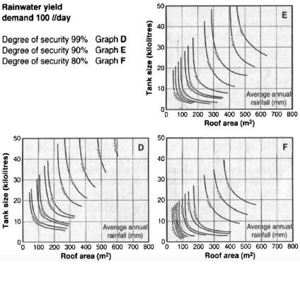
Methods to calculate the required storage capacity, varying in complexity and sophistication (McMahon & Mein, 1986), fall into three categories: simplistic approaches using annual rainfall totals, analytically derived equations, and continuous mass balance simulations. An example of the first is the method used by Gould (1999) to create curves defining the relationship between catchment area, storage size, annual rainfall total and the ‘degree of security’, as shown in Figure 3. The problem with such approaches is that by simplifying the local precipitation regime to its annual value, the complexity of this critical parameter is ignored. As Basinger et al. (2008) argue, the method assumes that the same tank size, would, in two locations with completely differing temporal rainfall distributions but same annual totals (such as NYC and Accra), provide the same reliability, all other parameters being equal. The second category includes analytically rigorous formulae, such as those derived by Guo and Baetz (2007), which apply stormwater detention theory and use numerous statistical characteristics to capture the complexity of rainfall (Hanson & Vogel, 2014). The third and most common approach is the use of continuous mass balance simulations, which aim to mimic the operation of a RWHS (Fewkes, 1999).
As explained by Su et al. (2008), the philosophy behind the mass balance method is that the “physical process of a system can be described through repeated system operations with pre-set parameters and an array of input data. System characteristics and behaviours can be better understood through the simulation process.” The operation of a RWH tank is discretised into time intervals. Inflow and outflow are then simulated, and the volume of water at the end of each interval is recorded and carried through to the next interval. The rainfall supply (discussed in section 4.2.2) is taken as the inflow into the tank, demand is taken as the outflow, and any excess inflow, limited by the capacity, is disregarded (Khastagir & Jayasuriya, 2010). In most cases a constant value for demand may be assumed (Lee, et al., 2000), especially if the RWHS is to be used for toilet flushing. Following Butler’s (1993) observation that the variation of WC usage on weekdays was low, Fewkes (1999) concluded that an average daily demand may be assumed, and that accurate modelling is only required if demand displays unusual daily variance.
Two types of mass balance algorithms exist: the yield-before-spillage (YBS) and yield-after-spillage (YAS) procedure. The former assumes that at the end of each time interval demand is withdrawn before spillage is removed, whilst the latter assumes the opposite (Liaw & Tsai, 2004). Since the YBS algorithm implies that the tank will be fuller after each time interval, the reliability calculated will be greater (Liaw & Tsai, 2004). Some studies opt for the more conservative YAS approach (Hanson & Vogel, 2014 ; Fewkes, 1999) whilst others chose the YBS method (Su, et al., 2009 Basinger, et al., 2010 Liaw & Tsai, 2004). In reality the behaviour (and consequently also reliability) of a RWHS will lie somewhere between the YBS and YAS approach, but the smaller the time interval used, the smaller the difference between both approaches and the more accurate the simulation becomes.
Different sets of equations have been used in previous studies to perform mass balance simulations but all rely on the principles discussed above. The equations below, except for (8), are used by Su et al. (2008). The authors start by defining the inflow of rainwater into the tank, using equation (5).
| It=Pt1000 × A | (5) |
t
subscript denotes the value of the parameter during or at the end of the
tth time interval.
It is the inflow (m3),
Pt the precipitation (
mm) and
A the catchment area (
m3). The quantity of water released by the storage tank is then determined using equation (6).
| Rt=Dtif St-1+It≥Dt St-1+Itif St-1+It |
(6) |
Dt
is the demand (
m3) and
St-1the quantity of water stored at the end of the previous time period (
m3). Thereafter, the quantity of spillage is calculated, using the YBS algorithm, as per equation (7).
| SPt=St-1+It-Dt-Smaxif St-1+It-Dt≥Smax 0if St-1+It-Dt |
(7) |
SPt
is the quantity of spillage (
m3), and
Smax the storage capacity (
m3). Equation (8) demonstrates what formula would had been used, had the authors opted for the YAS method.
| SPt=St-1+It-Smaxif St-1+It≥Smax 0if St-1+It |
(8) |
Finally, the quantity of water stored at the end of every time interval can be found using equation (9). For the first day of simulation some authors assume a full storage tank (Guo & Baetz, 2007) whilst others assume an empty one (Basinger, et al., 2010).
| St=Smaxif SPt≥0 St-1+It-Rtif if SPt<0 | (9) |
Thereafter, both temporal and volumetric reliability may be calculated as discussed in section 4.2.3.
4.2.5 Rainfall Series
The rainfall data used in mass balance simulations differs in terms of time intervals it is divided into, the data length, and whether the data used is historical or stochastically generated.
RWHS experience continuous inflows and outflows of water, but the level of detail with which system operation may be simulated is dependent on the level of detail of available rainfall data. Furthermore, although shorter time intervals for inflows and outflows will yield more accurate results, they also become more laborious. Heggen (1993) argued that the use of daily rainfall series provided more accurate results than weekly or monthly series, and Fewkes (1999) demonstrated that the difference in results between daily and hourly series was negligible. Thus, most studies opt for daily simulation intervals (Su, et al., 2009 ; Basinger, et al., 2010 ; Imtaez, et al., 2011 ; Liaw & Tsai, 2004 ; Hanson & Vogel, 2014 ; Rahman, et al., 2012). Nevertheless, some use monthly intervals (Ghisi, et al., 2007), whilst others use hourly (Villarreal & Dixon, 2005) or 5 minute (Coombes, et al., 2000) intervals.
Another question that arises is how long the rainfall record should be. Using a longer record length produces more realistic results (Su, et al., 2009), but also make simulations more computationally heavy. The recommended minimum length ranges between 20 (Khastagir & Jayasuriya, 2010) and 50 years (Liaw & Tsai, 2004). Most studies use the full length of available rainfall data, which may be up to 150 years (Rahman, et al., 2012), whilst a few studies restrict themselves to a subset of the available data. For instance, Basinger et al. (2008) mathematically defined the optimal length as that beyond which the marginal increase in complexity and computational labour outweighed the marginal increase in reliability, and concluded that 25 years was the optimal rainfall series length.
A final differentiating factor is whether simulators use historical data or stochastically generated data. The disadvantage of the former is that only one time period is considered and other possible precipitation scenarios, that could have occurred and may occur, are ignored (Basinger, et al., 2010). Furthermore, inaccurate estimates may be obtained if the life of RWHS exceeds the historical period used in analysis. Another advantage of stochastic generators is that they may be used to generate many synthetic series so that various reliability metrics, such as mean, minimum or 5th percentile values, may be computed. Basinger et al. (2008) argue that 100 generated rainfall sequences suffice to understand the distribution of reliability for a given set of parameters.
4.3 Stochastic rainfall generators
4.3.1 Overview
Stochastic weather models (or generators) produce artificial sequences of a certain variable, such as precipitation or temperature, that are statistically consistent with the historical record (Mehrotra & Sharma, 2007). Originally they were used to simulate weather series either in unobserved locations where historical data was unavailable, or in locations where existing historical data was too short to allow for hydrological risk assessments (Semenov & Barrow, 1997). As Sharma and Lall (1999) note, simulation models should be “capable of simulating sequences that represent the observed processes, are computationally robust, and are intuitively simple to understand.”
Stochastic precipitation generators are generally classified by the time intervals over which they simulate rainfall. Thus, three common categories include: annual, monthly and daily simulators (Srikanthan & McMahon, 2001). Annual generators analyse the frequency distribution of historical annual rainfall totals, fit a probability distribution to the data, and use the latter to generate artificial values. Monthly generators use the method of fragments, by which generated annual rainfalls are disaggregated and spread over twelve months (see section 4.3.2). As Srikanthan and McMahon (2001) note, little work has been done on the generation of annual and monthly precipitation series. Daily rainfall generators, inherently more complex, can be divided into 4 groups (of which the first two are the most popular): resampling models, two-part models, transition probability matrix methods and models of the ARMA type. The former comprises models that resample certain characteristics from a rainfall record (Mehrotra & Sharma, 2007). Two-part models first simulate rainfall occurrence, either by using continuous Markov chains to generate sequences of wet and dry days or by using alternating renewal processes to create series of wet and dry spells. Thereafter, they use probability distributions to generate rainfall amounts for wet days / spells (Srikanthan & McMahon, 2001).
Although RWH studies have used a variety of differing stochastic models the most common type is the daily rainfall generator, since most mass balance simulators use daily time intervals (see section 4.2.5). Basinger et al. (2012) developed a model using Markov chains to develop sequences of wet and dry days, but thereafter resampled daily rainfall amounts from the historical record. The authors argued that since their non-parametric resampling approach made no assumptions about the statistical form of precipitation, it was transferrable to new locations which would not have been the case for parametric models. However, the major disadvantage of such an approach is that, similar to the use of historical rainfall records, only rainfall amounts that previously occurred are considered. Cowden et al. (2008) used both types of 2-part models (continuous Markov chains and alternating renewal processes) to simulate daily rainfall, compared the results of the two, and concluded that each had its advantages, being able to better reproduce certain statistics.
4.3.2 Method of Fragments
The first step to using the method of fragments is to generate annual rainfall totals. Some generators (Thyer & Kuczera, 1999 ; Piantadosi, et al., 2009) assume that annual rainfall series can be described as a sequence of dry and wet years. Thus, these generators first use Markov models to develop a sequence of dry and wet years, and then use two distinct probability distributions (one for wet and one for dry years) to generate annual rainfall totals (Srikanthan & McMahon, 2001). Simpler approaches do not distinguish between dry and wet years and use a single distribution.
A wide array of probability distributions, which relate the magnitudes of annual rainfall to their likelihood of occurrence, may be chosen from, fitted to the data, and used to stochastically generate annual rainfall values. Most generators, such as those used by Thyer and Kuczera (1999) or Piantadosi (2009) use normal probability distribution functions, because longer aggregations of data tend to be best described by symmetrical distributions (Svensson, et al., 2017). Nevertheless, other distributions may better suit annual totals (Markovic, 1965). The most popular bivariate distributions for hydrological applications are the Generalised Logistic, Lognormal, Normal, Gamma and Weibull distributions (Svensson, et al., 2017). Several approaches for estimating distributions parameters exist, such as the moment matching or quantile matching estimation methods, but the most common method is the maximum likelihood method developed by R. A. Fischer, which optimises parameter values by maximising the log-likelihood (Markovic, 1965).
A variety of tests are used either to decide whether a fitted distribution accurately represents the data, or to choose the distribution that best fits the data. Visual assessments, comparing the quantiles or cumulative distribution of the actual data and fitted distribution, may be used as a rough indication of how well a distribution fits the data (Svensson, et al., 2017). More rigorous approaches involve the use of statistical goodness-of-fit tests, which quantify how likely a given distribution is representative of the data. A significance level (often around 5%) is chosen and if the test metric, the p-value, falls below this level, the distribution is rejected. Alternatively, when comparing several distributions, the one providing the highest p-value will be the one most likely to fit the data (Svensson, et al., 2017). Common tests include Kolmogorov-Smirnov (KS), Anderson-Darling (AD) and Cramér-von Mises (CM) tests. The KS is the simplest of these, and uses the maximum difference between the empirical and theoretical cumulative distribution function, derived from the observed data and fitted distribution respectively, to calculate the likelihood of fit (Piantadosi, et al., 2009). The CM is a refinement of the KS test, and was further modified to give the AD test, which gives more weight to the tails of distributions (Svensson, et al., 2017). Previous RWHS studies (Guo & Baetz, 2007 ; Basinger, et al., 2010) use both the KS and AD tests to verify the distribution of rainfall.
After the most appropriate distribution has been fitted and a series of annual rainfalls has been generated, the series may be disaggregated into monthly values. Known as the method of fragments and first used by Srikanthan and McMahon in 1985, this method involves analysing the historical data, and for each year calculating the fraction of annual precipitation that fell in each month, thus giving 12 fragments per year (Srikanthan & McMahon, 2001). Each generated annual total is multiplied by a set of fragments selected at random, to give 12 monthly rainfalls. The main shortcoming of this method is that the correlation between the last month of one year and first month of the following year will not be preserved. However, this issue may be mitigated by using a hydrological year whose start and end is defined by the two consecutive months marked by the smallest serial correlation.
4.4 RWH in the UK
4.4.1 Importance & Use
RWHS are becoming increasingly important in urban areas of developed countries. The growing water demand, rising flood risk due to increasing surface run-off, and large infrastructures required to transport water to these areas of high demand, have put centralised water supply and disposal networks in urban areas under increasing stress (Pratt, 1999 ; Geiger, 1995). These problems are especially pronounced in the UK, where regions of high water demand, such as London, are categorised as having “very low” water availability (Fewkes, 2012). To make matters worse, the government’s Sustainable Communities Plan announced that 4.8 million new homes would be constructed between 2006-2026, 60% of which will be built in areas where water is scarce (Fewkes, 2012). To mitigate the potential problems, the government announced their aim to reduce daily per capita domestic water consumption from
150L to
130L (Environment Agency, 2010).
Unfortunately, compared to other developed countries, the UK has failed to promote the use of RWHS on a large scale (Berndtsson, 2004). In Australia and New Zealand, the use of RWHS is strongly encouraged – Australia even went so far as to introduce legislations, making it a requirement for new-builds in some regions (such as Sydney) to have rainwater tanks (Rahman, et al., 2012). In the USA, 100,000 RWHS are estimated to be in use (Fewkes, 2012). In Germany, charges related to domestic water supply and discharge have been adapted to provide financial incentives for owners to install RWHS (Hermann & Schmida, 2000). Although the number of RWHS being installed in the UK annually has increased to 7,500, it is evident that it is falling behind when compared to a country like Germany, where 50,000 systems are installed annually, (Fewkes, 2012).
4.4.2 UK Sizing Guidelines
The BS, the official UK guideline for the design of RWHS, covers topics such as the sizing of tanks for non-potable domestic use or storm water management, various system types, system installation, operation and maintenance. To determine the required storage capacity for domestic use it offers three methods: the simplified, intermediate or detailed approach (British Standards Institution, 2009).
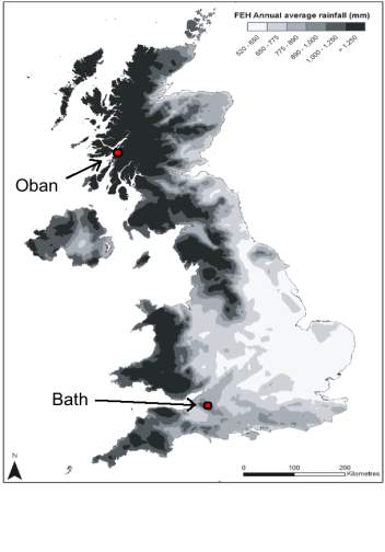
The simplified method, which is to be used for residential properties and assumes a consistent daily demand of 50L/person/day for WC flushing and clothes washing, first requires the designer to use an annotated map (Figure 27; displayed and used in section 7.2) to determine the average annual rainfall depth for their location. Thereafter, given the number of persons per household, the roof plan area and the average annual rainfall depth, graphs can be used to determine the recommended storage capacity (Figure 28; also displayed and used in section 7.2). The BSclaims that by applying this method, around 80% of runoff will be utilised.
The intermediate approach, similar to the simplified method, makes use of equations to calculate the required storage capacity. It states that the storage capacity should be the less of either a) 5% of the annual rainwater yield or b) 5% of annual non-potable water demand. These two values may be calculated using equations (10) and (11).
| YR=A × e × AAR × h × 0.05 | (10) |
| DN=Pd × n × 365 × 0.05 | (11) |
In equation (10),
YR is 5% of the annual rainfall (L),
A the catchment area (m2),
e the yield coefficient (%),
AAR the annual average rainfall depth for the given location (mm) and
h the hydraulic filter efficiency (%). For equation (11),
DN is 5% of the annual non-potable water demand,
Pd is the daily per capita demand (L) and
n is the number of persons.
Finally, the detailed approach is meant for “very large schemes where significant economic savings might be achieved or where daily demand or seasonal rainfall is quite variable.” It suggests using continuous rainfall time series, but does not provide further guidance on how such an analysis should be carried out.
The key disadvantage of the BSis that it fails to deliver an approach which considers: the seasonal variation in rainfall, the reliability that a certain storage tank will provide, and how climate change will affect system performance in the future. The simplified and intermediate approach neglect both these factors all together. Consequently, although a house owner who wishes to install a RWHS could use the BSto determine the recommended storage capacity, they will not know with what reliability the RWHS will be able to meet the domestic non-potable water demand.
4.4.3 UK RWH Parameters
To create location-specific graphs relating demand, catchment area, storage capacity and reliability, representative values of these parameters for the UK must be known.
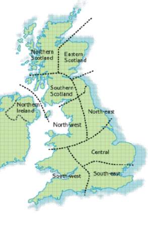
UK rainfall data is published online by the UK MET Hadley Centre. The website provides both location specific data, such as for Heathrow, and regional data, by dividing the UK into nine areas (as shown on Figure 4) and providing representative precipitation values for these.
The average daily domestic per capita water demand lies at 150L. Non-potable uses, such as toilet flushing, clothes washing and outdoor use represent 26%, 12% and 7% respectively (Environment Agency, 2010). However, most studies consider the use of RWHS solely for toilet flushing and clothes washing only, and assume these represent roughly one third of the domestic demand (Fewkes, 2012), thus giving a daily per capita demand of 50 L, which RWHS are designed to cater for (British Standards Institution, 2009).
Two of the most popular RWHS suppliers, Alumasc and Kingspan, provide storage tanks ranging from 1500L to 5000L (Alumasc Rainwater Services, 2010) and 1500L to 4600L (Kingspan Water, 2013) respectively. Khastagir and Jayasuriya (2010) note that domestic tank sizes rarely exceed 5000L. The Kingspan company brochure recommends their largest tank for roof sizes of circa 200m2, therefore it can be assumed that most residential homes will have roof areas below this value.
4.5 Climate Change Impact on Precipitation
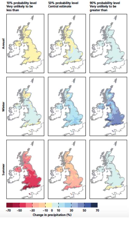
Many differing predictions for how climate change will affect precipitation have been proposed, but most agree that precipitation variance is likely to increase globally (Dore, 2005). In other words, wet areas will become wetter; dry areas drier. As such, it is expected that rainfall over Northern latitudes will increase 0.5% – 1% per decade.
The 2009 UK Climate Change Projections (UKCP09) present possible future weather scenarios (Defra, 2009). The UKCP09 are based on numerous weather simulations (Defra, 2011), which draw on the IPCC’s (Intergovernmental Panel on Climate Change) low-, medium- and high-emission projections. Three scenarios are presented: the 10th percentile (dry scenario), 50th percentile (median / central scenario) and 90th percentile (wet scenario) results.
Figure 5 shows these scenario changes for annual, winter and summer precipitation. For the central estimate, there is no clear change in annual precipitation, but summers are expected to become drier, especially in the South West of the country, and winters are anticipated to become wetter.
5 Methodology
5.1 Overview and Rationale of Approach

The first step consisted of creating a stochastic monthly rainfall generator. For a given location this generator analysed the distribution of historic annual rainfall, fitted a probability distributions, and then used this to generate sequences of synthetic annual precipitation values. To obtain a series of monthly rainfalls, a procedure similar to the method of fragments was used.
The stochastic generator was developed because it enabled the study of RWH reliability not only for the historic rainfall series, but for possible rainfall scenarios that could have occurred and might still occur. Furthermore, by generating many rainfall series and calculating the reliability for each, the distribution of reliability for a given set of parameters may be understood.
A monthly, as opposed to a daily, rainfall generator was developed for two reasons. First, daily rainfall generators are far more complicated (as discussed in 4.3.1). More importantly, the focus of this study was not to develop the most complex rainfall generator possible, as this would require input from a rainfall modelling expert. Rather, the aim was to investigate the relationship between the reliability, storage capacity, catchment area and demand, and demonstrate how the graphs produced may be used as part of a reliability-based design approach. As such, for the purposes of this dissertation, a monthly rainfall generator was deemed to be sufficient.
A mass balance simulator was then used to calculate the temporal and volumetric reliability for each of the generated monthly series, for various parameter combinations. Thus, for each parameter combination, numerous reliability measures were found (one per sequence), and reliability statistics, such as the mean, 5th percentile or 95th percentile, could be calculated.
Mass balance simulations using historical monthly and daily series, and historical and generated monthly series, were also undertaken, the former to assess the impact of time intervals on simulation results, the latter to test the accuracy of results and using the generated series.
Finally, the UKCP09were used to modify the generated monthly rainfall series to create three sets of possible sequences, corresponding to the 2080 dry, median, or wet scenario. Reliability for these were then again calculated using mass balance simulation to deduce how future reliability values might differ.
Figure 6 summarises the methodology. To explain the procedure and analysis conducted, the following sections will use SWEaWand NSas regional examples, because they have differing precipitation regimes and because climate change is predicted to impact rainfall in these regions in different ways. Tables and figures presented will alternate between these two regions. Usually, such illustrations will only be presented for one of the regions to avoid repetition, unless it is deemed that reference to both is necessary.
5.2 Defining the Hydrological Year
First, the start and end of the hydrological year had to be defined by the two consecutive months marked by the smallest serial correlation. As argued by Srikanthan and McMahon (2001), this helps minimise the discontinuity between the first month of one year and the last month of the previous year, when using the method of fragments.
Several tests exist that quantify the correlation between two variables, such as those devised by Pearson, Kendall or Spearman. The first is used when the two variables are from a normal distribution, the second when they do not necessarily come from a normal distribution, and the third when they do not stem from a normal distribution (Kassambara, 2015). Thus, Kendall’s correlation coefficient was used identify the two consecutive months with the lowest correlation, since no studies were conducted on the distribution of monthly rainfall.
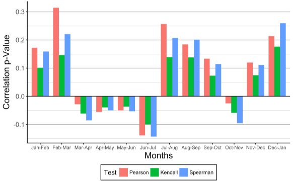
Figure 7: Bar chart of correlation values between consecutive monthly rainfall values for NS
Figure 7 shows the correlation values for consecutive monthly rainfall totals in NS. Results show that the two months marked by the lowest correlation, as calculated by the Kendall test, are May and June, followed closely by April and May. For SWEaW, the two months with the lowest correlation were January and February.
5.3 Fitting Probability Density Functions to Annual Rainfalls
Once the historic monthly rainfall data was rearranged as per the defined hydrologic year, annual rainfall totals were calculated to obtain series of annual rainfall totals for the studied locations.
Since rainfall is a random process, the frequency distributions of these annual rainfall totals were analysed to understand their magnitude-dependent probability of occurrence. This allowed to model probability density functions which were then be used for the generation of rainfall series. This process can best be understood by depicting annual rainfall as a histogram and superimposing the fitted probability density function, as shown in Figure 8.
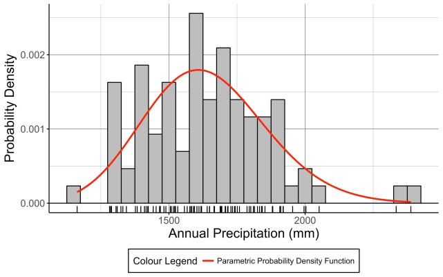
Figure 8: Annual precipitation histogram and fitted Normal probability density function for NS
To model the probabilistic distribution, five bivariate functions often used in hydraulic applications (as mentioned in section 4.3.2) were considered: the Normal, Gamma, Lognormal, Weibull and Generalised Logistic distributions. To determine which of these could best be used to represent the data, the AD test, which was selected for its use in previous RWH studies and its advantages over other tests (as discussed in section 4.3.2), was used. Fitting these distributions to the data and then using the same data to assess the fit would not have been appropriate since the fitted distribution would have been biased towards the data – a phenomenon known in statistics as ‘overfitting’ (Deane-Mayer & Kuhn, 2015). Thus, the method of cross-validation was used: 80% of the data was selected at random to fit the distribution, and the remaining 20% was then used to assess the fit by calculating the p-value. Since the fit and test data were selected at random, each test yielded a different p-value. With an increasing number of tests the average of these p-values converged. For this study, cross-validation and testing were performed 10,000 times for each distribution, and the one with the highest average p-valueas per the ADtest was selected. The Normal and Gamma distributions were chosen for NS and SWEaW respectively. The distribution parameters were then fitted using the maximum likelihood estimation method.
5.4 Generating Monthly Rainfall Series
For each location, the fitted probability distributions were used to generate 100 synthetic annual rainfall series, each the same length as the historic series (143 and 85 years for SWEaWand NS respectively). 100 sequences were generated because, as discussed in section 4.2.5, this quantity provides sufficient reliability values to understand their distribution for a given combination of parameters. The sequences were generated to the same length as the historic data so that when comparing reliabilities obtained using the historic and stochastic rainfall series, the assumption of the tank being empty at the start would have the same effect on both reliability values. Another benefit of having series the same length is that their quantiles may easily be plotted against each other to assess the fit of the theoretical distribution (demonstrated in section 6.1.1).
The generated rainfall sequences were then disaggregated into monthly values. However, instead of randomly choosing a set of fragments from the complete historical record, as proposed by Srikanthan and McMahon, and reviewed in section 4.3.2, only a subset of the historical record was considered. Solely the sets of fragments derived from the 20% of historical annual totals whose values were closest to those of the artificial annual total, were used. One year was then selected at random from this subset, and its set of fragments (of monthly rainfalls as a fraction of the annual rainfall) was used to disaggregate the generated annual value. The rationale behind selecting a set of fragments from a smaller subset is that this would better conserve any patterns related to the monthly distribution of rainfall as a function of the annual total. However, limiting the subset to a smaller fraction of the complete record (for instance 5%) would have resulted in some odd patterns appearing in the generated monthly rainfall series, as shown in section 6.2.
5.5 Calculating Current Reliability
To calculate the reliability provided by a certain storage size for a given set of parameters, mass balance simulations were performed. A YBS algorithm was used, and it was assumed that the storage tank was empty at the start of simulation. Representative UK parameter values were considered: catchment areas ranging between
0 to 200m2,
storages of 1500L, 3000L and 5000L,
and daily demands of 100L and 200L (corresponding to 2-, and 4-persons households).
All possible parameter combinations were then arranged in a matrix, each row in the matrix corresponding to one combination.
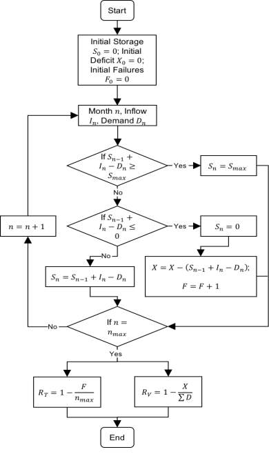
For each location, and each parameter combination, the historic daily, historic monthly and 100 generated monthly rainfall series were fed into the mass balance simulator to calculate three types reliabilities: a single historic daily reliability, a single historic monthly reliability, and an array of 100 monthly stochastic reliabilities. Furthermore, for each of these, reliability was calculated both temporally and volumetrically (explained in section 4.2.3). The computer algorithm developed to simulate system behaviour and calculate reliability may be visualised as a flowchart as shown in Figure 9.
5.6 Incorporating Effects of Climate Change
To predict how reliability might be altered by climate change, the UKCP09were used to estimate the seasonal percentage change in rainfall under 2080 dry, median or wet scenarios. Figure 5 (section 4.5) was used to approximate the average percentage change in winter and summer precipitation in NS and SWEaW, as summarised in Table 1. These seasonal changes were then modelled on a monthly basis, by taking January and July as the centres of winter and summer respectively, and assuming that the percentage change would vary sinusoidally between these two months.
Table 1: Percentage changes in winter and summer rainfall for dry, median and wet scenario in SWEaW and NS
| Dry Scenario | Median Scenario | Wet Scenario | ||||
| SWEaW | NS | SWEaW | NS | SWEaW | NS | |
| Winter (January) | 0% | 0% | 20% | 25% | 50% | 50% |
| Summer (July) | -60% | -35% | -30% | -15% | 0% | 0% |
Figure 10 shows the monthly percentage change in precipitation for SWEaW. Note that only percentage change values for January and July were taken from Figure 5 (UKCP09 projections), and the remaining values were calculated by assuming a periodic fluctuation as shown.
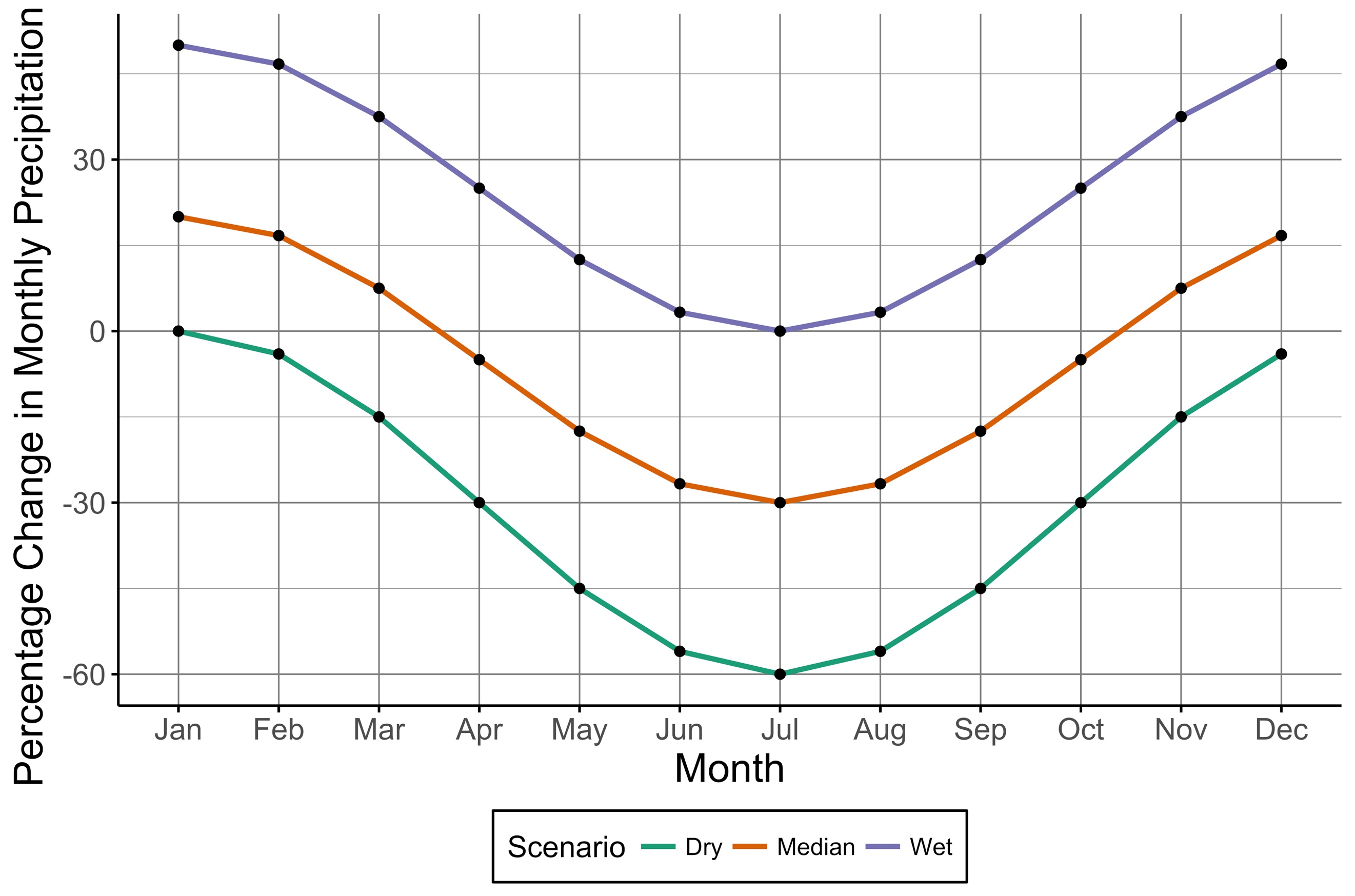
Figure 10: Percentage change in monthly precipitation for 2080 dry, median and wet projections in SWEaW
The generated monthly series were then modified by applying the percentage changes as per Figure 10. Thus, three sets of generated rainfall series, each containing 100 sequences, were obtained, which represent potential rainfall series in 2080 under the three possible scenarios. Figure 11 depicts the mean monthly rainfalls in SWEaW from all four stochastic monthly rainfall series: the current, the 2080 dry, the 2080 median and the 2080 wet rainfall sequences. When comparing with the current generated series, the future dry series has less than or similar monthly rainfall, the wet series has greater than or similar monthly rainfall, and the median series has higher and lower mean rainfall in winter and summer months respectively.
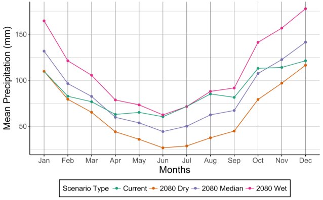
Figure 11: Mean monthly precipitation values for current and future stochastic rainfall series in SWEaW
These future rainfall series were then fed into the mass balance simulator, which calculated reliabilities for the future rainfall scenarios. The simulation relied on the same assumptions and those outlined in section 5.5.
6 Discussion and Analysis of Results
6.1 Accuracy of Stochastic Rainfall Series
Since the aim of rainfall generators is to simulate artificial rainfall that is representative of the observed data, testing the statistical similarity between the observed and generated data is necessary to determine whether the latter is accurate enough for design purposes. Hence, the similarity between historic and generated annual and monthly rainfall series was analysed.
6.1.1 Accuracy of Annual Stochastic Rainfall Series
The p-values obtained from both the KS and AD test may be used as an indication for how likely a distribution is to accurately represent the data. Table 2 shows the values obtained for SWEaW. As mentioned in section 4.3.2, a common significance level in hydraulic applications is 0.05. The p-values obtained, lying significantly above 0.05, suggest that all distributions could be used to model annual rainfall, but that the Gamma distribution (in bold) has the highest probability of fit. For NSthe Normal distribution was chosen, with an ADp-valueof 0.474.
Table 2: Distribution goodness-of-fit tests to model annual rainfall in SWEaW
| Normal | Gamma | Weibull | Lognormal | Logistic | |
| KS p-value | 0.479 | 0.483 | 0.469 | 0.482 | 0.462 |
| AD p-value | 0.473 | 0.474 | 0.450 | 0.470 | 0.472 |
The distribution of historic and generated annual rainfall may be compared using visual plots. Overlaying the fitted distribution onto the histogram of observed data, as shown in Figure 8, may be used as an indication of fit, but histograms vary with bin width and consequently the perception how well a distribution represents the observed data may change. Therefore, plots comparing empirical and theoretical cumulative probability functions or quantiles, are better alternatives. Figure 12 is an example of the former for SWEaW. The closer the black points (empirical) lie to the modelled cumulative probability density function (using a Gamma distribution), the better the fit.
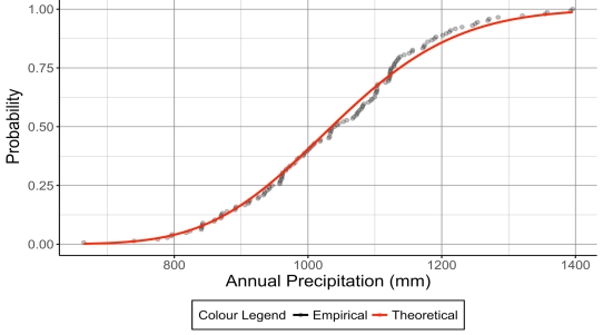
Figure 12: Empirical and theoretical cumulative probability functions for annual rainfall in SWEaW
Figure 13 shows the theoretical quantiles derived from the fitted Gamma distribution plotted against the quantiles from the observed data set. A perfect fit would be displayed by all quantiles lying on the straight line y=x, where x and y are the two axes. It may be observed that the quantile plot displays an outlier towards the top right of graph. This could suggest that the theoretical distribution slightly overestimates high annual rainfall values. However, since this trend may only be observed for one value it is not a major concern.
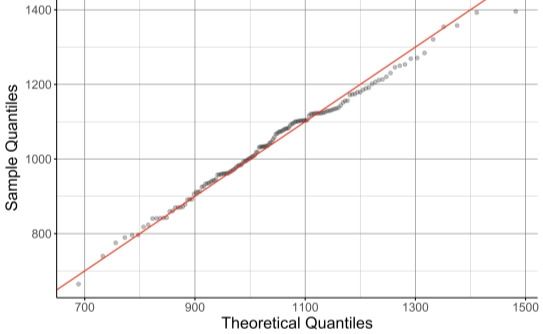
Figure 13: Sample and theoretical quantiles of annual rainfall in SWEaW
Figure 12 and Figure 13 display strong similarity between theoretical and empirical cumulative probability distributions and quantiles, which indicate that the modelled Gamma distribution accurately represents the annual distribution of rainfall in SWEaW.
6.1.2 Accuracy of Monthly Stochastic Rainfall Series
Box plots, also known as whisker plots, provide a meaningful and easy to understand method for comparing data series. These typically display five values: the median (50th percentile), lower quartile (25th percentile), upper quartile (75th percentile), minimum and maximum value. Using extremes (minimum and maximum values) to compare the historic and stochastic monthly rainfall series would have been inappropriate since the stochastic rainfall series comprise 100 sequences, and is therefore more likely to include extreme values. Hence, 5th and 95th percentile values were used to mark the lower and upper bounds of the boxplot, respectively. Figure 14 displays the boxplot for SWEaW. Generally, there is a strong similarity between the generated and historic rainfall quantiles, which leads to the conclusion that the monthly rainfall generator is accurately able to replicate the historical rainfall series.
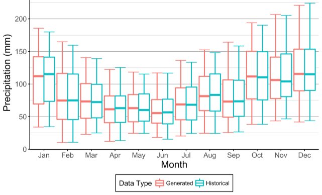
Figure 14: Boxplot of generated and historical monthly precipitation for SWEaW
6.2 Method of Fragments: Impact of Subset Size
To disaggregate a generated annual value, only the fragments derived from the 20% of historic annual values whose magnitudes were closest to the generated annual value, were considered. To choose this fraction (20%), scatter plots showing the generated and historical monthly rainfall values were used.
Figure 15 and Figure 16 show the scatter graphs produced by using 5% and 100% of historic annual values for disaggregation, respectively, for NS. The generated points were made transparent so that their degree of overlap may be deduced. The generated monthly series for the first graph are marked by an odd phenomenon: the scattered points representing generated monthly values seem to cluster thereby forming distinct stripes. In other words, generated monthly rainfall values tend to fall within certain ranges. This unrealistic phenomenon could lead a person, looking at Figure 15, to conclude that during June, the monthly rainfall depth cannot lie between 170 and 200mm. The cause of this unrealistic distribution of monthly rainfall values is the limited set of fragments used to disaggregate the data. Only 4 (or 5%) of the 85 years of data for NS were considered for each disaggregation, and no combination of generated annual rainfall multiplied by a randomly selected set of fragments (from a total of 4 sets) gave a monthly precipitation between 170 and 200mm in June. Thus, this unrealistic phenomenon can be mitigated against by considering more sets of fragments for disaggregation, as shown by Figure 16.
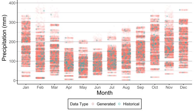
Figure 15: Scatter plot of monthly rainfall for historical and generated rainfall series (using 5% of sets of fragments) in NS.
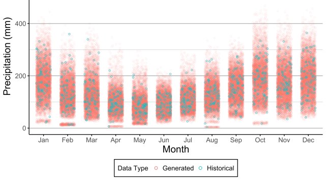
Figure 16: Scatter plot of monthly rainfall for historical and generated rainfall series (using 100% of sets of fragments) in NS.
This phenomenon may also be visualised using violin plots as shown in Figure 17 and Figure 18, again produced by using 5% and 100% of historic annual values for disaggregation, respectively, for NS. The area of violin plots remains constant, but their thickness corresponds to the distribution density for that given monthly rainfall value. Ideally, the plot created from the generated data should match the underlying historical plot. In Figure 17, the abrupt fluctuations in thickness for the generated series reflect the tendency for generated values to cluster within certain rainfall ranges when using a smaller quantity of sets of fragments for disaggregation. By increasing the sets of fragments considered, as shown in Figure 17, this problem may be mitigated against.
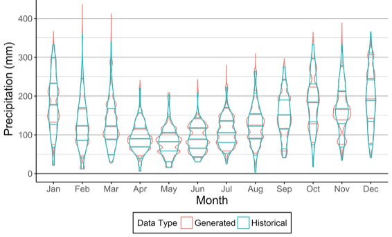
Figure 17: Violin plot of monthly rainfall for historical and generated rainfall series (using 5% of sets of fragments) in NS.
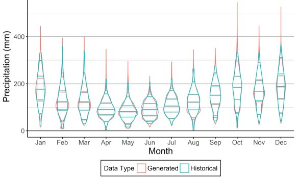
Figure 18: Violin plot of monthly rainfall for historical and generated rainfall series (using 100% of sets of fragments) in NS.
However, by using a greater set of fragments, patterns related to the monthly distribution of rainfall as a function of the annual total, may not be conserved. For instance, if large annual precipitation totals were primarily the result of high rainfall in January and February, using all available sets of fragments for disaggregation, as opposed to only those derived from years marked by high annual rainfall, could result in the failure to incorporate this trend into the generated rainfall series.
Thus, choosing the quantity of sets of fragments for disaggregation is a balance between mitigating against the unrealistic distribution of monthly rainfall values, and incorporating patterns related to the monthly distribution of rainfall as a function of the annual total. To disaggregate generated annual rainfall series for this study it was decided that 20% of sets of fragments should be considered, as the generated values no longer seemed to form distinct stripes when plotted on a scatter graph.
6.3 Assessment of Reliability
6.3.1 Comparison of Volumetric and Temporal Reliability
Figure 19 shows how temporal and volumetric monthly reliability vary with catchment area, storage capacity and daily demand, for SWEaW. Reliabilities were calculated using the stochastically generated monthly rainfall series. The graphs clearly demonstrate that the monthly temporal definition of reliability is more conservative than the volumetric alternative. This is because the former only considers whether a system was adequate or inadequate at the end of every time interval. For instance, if for a given monthly series a RWHS was able to meet 99% of the demand every month, the system would have a volumetric reliability of 99%, but a temporal reliability of 0%.
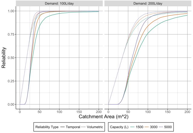
Figure 19: Volumetric and temporal reliabilities using generated monthly rainfall series for SWEaW
Which of the two reliability definitions is more suitable depends on whether the residence, for which the RWHS is to be designed, has access to a centralised water infrastructure. If it does, any rainwater deficit can be provided by this additional supply; if it does not, rainwater shortage can have severe consequences. For the former, volumetric reliability would be more meaningful since it provides an indication of centralised water volume and cost savings. For the latter, temporal reliability would be more appropriate since it provides a measure of risk. Since almost all UK residences are connected to a centralised water network, the volumetric definition of reliability is more suitable, and will be used in the following sections.
From Figure 19 it may also be observed that changes in storage capacities have a much greater impact on temporal reliability than volumetric reliability, which would suggest that storage size is not a key determinant of volumetric reliability. However, such a conclusion would be ill-founded as discussed in the following section (see section 6.3.2).
6.3.2 Comparison of Monthly and Daily Reliability
To calculate reliability from daily rainfall series (henceforth referred to as daily reliability), historic data was used since the rainfall generator developed only creates monthly rainfall series. Therefore, historic monthly rainfall series were used (as opposed to generated monthly series), to ensure that the comparison between daily and monthly reliabilities would not be dependent on the rainfall generator’s accuracy.
From Figure 20 it may be observed that the calculated reliability is greater when using the monthly rainfall series. This is because the monthly mass balance simulations only consider spillage of excess rainwater at the end of the month, whereas the daily mass balance simulations consider spillage on a daily basis. As such, a greater quantity of rainwater will be lost due to spillage in the daily simulations, which results in a lower system reliability. Furthermore, the smaller the storage capacity, the less rainwater the tank may store at any point in time, and the greater the amount of spillage. Therefore, the difference between daily and monthly reliabilities is more pronounced for smaller storage capacities, where the importance of accurate spillage modelling is more important.
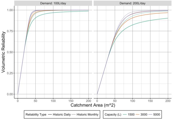
Figure 20: Daily and monthly reliabilities using historic rainfall series for SWEaW
Figure 20 also shows that changes in storage capacity have a greater impact on daily reliability. Thus, the hypothesis that volumetric reliability is only marginally affected by storage capacity, proposed in section 6.3.1, no longer holds. Rather, storage capacity is not a key determinant of monthly volumetric reliability, but is significant for daily volumetric reliability. Thus, the question which of the two reliabilities is the more meaningful arises.
As discussed in section 4.2.5, the smaller the time frame used in the mass balance simulation, the more accurately the simulation replicates real system behaviour, the more accurate the calculated reliability. Hence the daily reliability is the preferred measure, but for reasons discussed in section 5.1 only a monthly rainfall generator was developed. Thus, the following sections will only use monthly series to calculate reliabilities.
6.3.3 Comparison of Historic and Generated Reliability
As shown in Figure 21, reliabilities obtained from historic and stochastically generated monthly rainfall sequences (henceforth referred to as historic and generated reliabilities), are practically identical. As shown in Figure 22, the historic reliability seems to slightly exceed the generated one, although this difference is negligible. The historic reliability lies well within the grey area, representing the 90% confidence interval (using 5th and 95th percentiles as the lower and upper bound respectively) of generated reliabilities. Therefore, it may be concluded that the generated series can be used to accurately calculate monthly reliability.
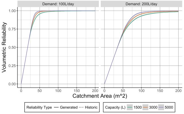
Figure 21: Generated and historic monthly reliabilities for SWEaW
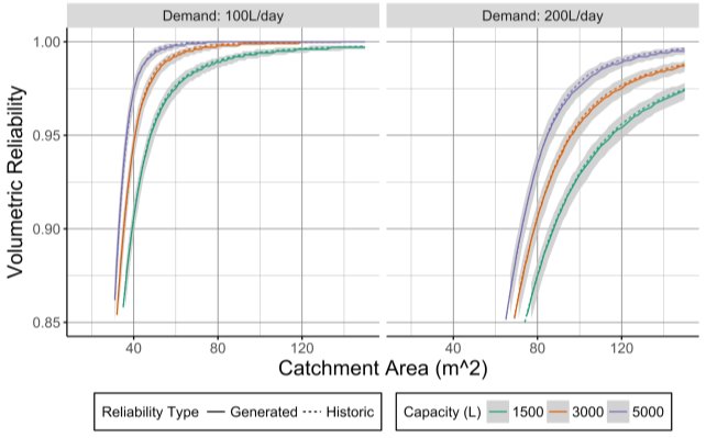
Figure 22: Enlargement of Figure 4.3.3-1
6.4 Reliability in 2080
The following section will display monthly reliability plots featuring the mean reliabilities calculated using the generated rainfall series for the present-day scenario (henceforth referred to as current reliability), and the generated rainfall series for the future dry, median or wet scenarios (henceforth referred to as dry, median or wet reliabilities).
It is worth mentioning that dry, median and wet scenarios were derived from climate change projections using a probabilistic approach. Since the dry and wet scenarios correspond to 10th and 90th percentile simulation results, there is a 10% probability that by 2080 rainfall may decrease or increase more severely than indicated by the dry or wet scenarios respectively. As such the dry and wet scenarios could be read as an 80% confidence interval around the median scenario (as will be done later in section 7.4), but when mapping several storage capacities, the overlap of confidence intervals would have made such graphs impractical and messy. Therefore, the following section covers these scenarios separately.
6.4.1 Dry Scenario
Under the dry scenario, RWHS see a considerable reduction in reliability. This is true for both SWEaWand NS, but especially for the former, as shown in Figure 23, since this region is predicted to experience a sharper percentage decrease in summer rainfall.
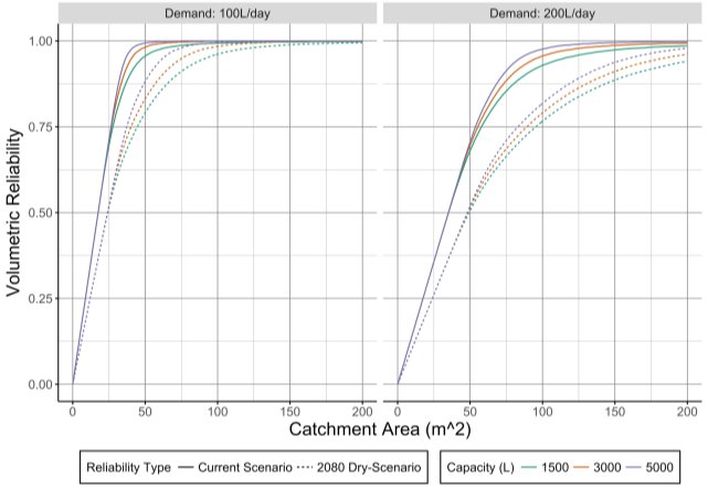
Figure 23: Current and future dry-scenario reliabilities for SWEaW
6.4.2 Wet Scenario
Under the wet scenario, the opposite occurs: RWHS reliability increases, as shown in Figure 24. However, it may quickly be observed that this favourable increase in reliability is much smaller than the adverse decrease in reliability as seen in the previous scenario.
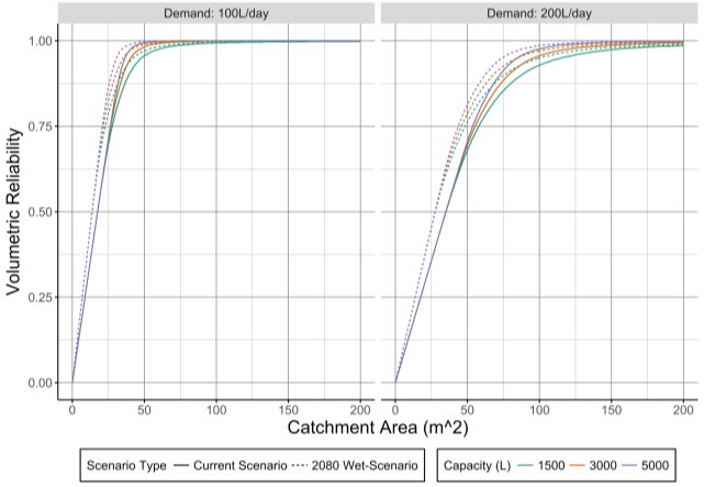
Figure 24: Current and future wet-scenario reliabilities for SWEaW
6.4.3 Median Scenario
As seen in Figure 25 and Figure 26, the median scenario shows a decrease in RWHS reliability, except for small catchment areas in NSwhere reliability is slightly increased. This might be because for NSthe predicted 25% increase in winter rainfall and 15% decrease in summer rainfall Table 1 result in both increased mean annual rainfall and seasonal variability, the former increasing RWHS reliability but the latter making it more difficult to achieve high reliabilities. It may also be observed that, as expected, reliability is forecasted to decrease more substantially in SWEaW than NS, since the rainfall regime for the former is more adversely affected.
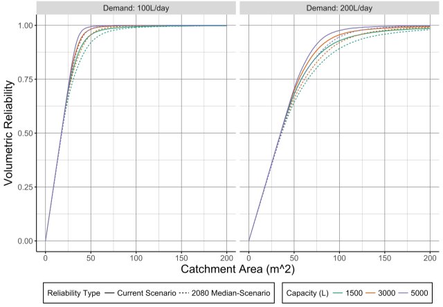
Figure 25: Current and future median-scenario reliabilities for SWEaW
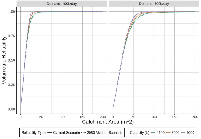
Figure 26: Current and future median-scenario reliabilities for NS
7 Case Study
7.1 Overview
In the following section the simplified and intermediate methods presented in the BSwere used to size RWH tanks in Bath (SWEaW) and Oban (NS). The volumetric reliability graphs using generated monthly series, presented in the previous chapter, were then used to assess what reliability the recommended storage sizes would provide under present-day and future rainfall scenarios. Thereafter, it was demonstrated how the graphs could be used for design to determine parameter combinations required to achieve a desired reliability.
For the case study a 4-person house with a pitched roof and plan area of 60m2 (3-floor house with 180m2 internal area) was assumed. As per the BS, daily per capita water demand was taken as 50L, the yield coefficient as 0.9 (for pitched roofs), and hydraulic filter efficiency as 0.9.
7.2 Simplified Approach
The mean annual rainfall in Bath, as per Figure 27, lies between 890-1000mm/year. For Oban, it exceeds 1250mm/year.
According to Figure 28 the recommended storage sizes for Bath and Oban are 1.9kL and 3.3kL respectively.
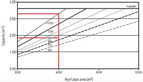
Figure 28: Simplified approach storage sizing graph for 4-person household (BS 8515)
7.3 Intermediate Approach
As outlined in section 4.4.2 the intermediate approach involves using equations to calculate 5% of the annual rainwater yield and 5% of annual non-potable water demand. The smallest of these two is then taken as the recommended storage size. Average annual rainfall values (between 1981-2010) for Bath and Oban were taken from the MET website as 814mm/year and 1680mm/year, respectively (MET Office, 2017).
Table 3: Recommended storage capacities as per intermediate approach (BS 8515)
| 5% of Annual Yield (L) | 5% of Annual Non-Potable Water Demand (L) | |
| Bath | 1978 | 3650 |
| Oban | 4085 | 3650 |
Table 3 displays the intermediate approach calculation results, and corresponding recommended storage size are highlighted in bold. The results obtained from the simplified and intermediate approach are very similar: for Bath the two are almost identical, and for Oban the intermediate approach recommends a storage ~10%greater than simplified approach.
7.4 Corresponding Reliabilities and Discussion
Since storage tanks come in standard sizes, 2000L and 3500L tanks were assumed for Bath and Oban respectively.
Figure 29 shows a reliability plot using generated monthly rainfall for present-day and future 2080 scenarios. The future median-scenario is shown by the dashed line, and the 80% confidence interval is shown by the surrounding grey area, whose lower and upper limits corresponds the dry and wet scenarios respectively.
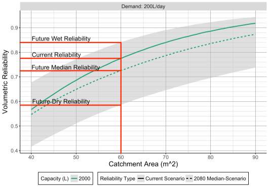
Figure 29: Enlargement of graph depicting current and future monthly reliabilities for SWEaW
Currently, a 2000L tank in Bath would provide a volumetric monthly reliability of 78%. By 2080, there is an 80% probability it will lie between 58% and 84% (corresponding to dry and wet scenarios respectively), and according to the central estimate it will have dropped to 72%. A similar analysis in Oban (with a 3500L tank) suggested monthly reliabilities of 96%, 88%, 95% and 98% for current-, future dry-, future median- and future wet-scenarios.
In both regions, a RWHS could be highly effective: In Bath three quarter of the non-potable water demand could be met, and in Oban practically all of it. Future changes in reliability are more uncertain in SWEaW than in NS, although central estimates agree that reliability is expected to decrease in both regions.
Figure 30 shows the reliability derived from generated present-day monthly rainfall series in SWEaW. The lines show mean reliability values, and the grey contours represent 90% confidence intervals (explained in section 6.3.3), although the boundaries of these become indiscernible at smaller catchment areas due to overlap. Maps such as these can aid residents in adopting a reliability based approach for optimising system parameters. For instance, should the residents in Bath desire a higher reliability they could install a 4000L tank to increase reliability to 80%. A more effective method, but more difficult to implement, would be to increase the roof / catchment area to 70m2, which if combined with a 4000L tank, would provide a reliability of 87%.
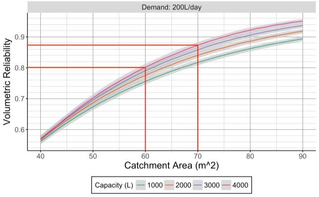
Figure 30: Enlargement of graph depicting current monthly reliabilities for SWEaW
8 Conclusion
This dissertation aimed to produce regional graphs for the UK relating key parameters that affect RWHS reliability: catchment area, daily demand and storage capacity. Thereafter, the potential effects of climate change were incorporated into these graphs to determine how reliability might change in the future. These accessible graphs allow UK residents to either quickly size storage capacities for a desired reliability, or understand what reliability a recommended storage size will provide. Although the graphs produced were limited to a few daily demand and storage capacity values since they were used for demonstration, they could be reproduced for any parameter values.
RWH was chosen as a field of study because of its numerous advantages and its potential effectiveness, irrespective of geographical location, as demonstrated by many studies. The scope was limited to the UK because it has failed to embrace the use of RWHS and because its urban population growth is putting centralised water infrastructures under increasing stress. The study focused on investigating the relationship between reliability and system parameters for present and future climatic conditions, because current UK guidelines fail to address reliability as a design parameter and ignore how climate change might impact system performance.
After developing a stochastic monthly rainfall generator and a mass balance simulator, the generator and various reliability measures were investigated. The accuracy of annual and monthly rainfall series, and the effects of changes in important model parameters, such as the number of historical years considered for monthly disaggregation, were examined. Thereafter, reliability graphs were used to compare: volumetric and temporal reliability, reliability derived from monthly and daily series to determine the impact of time intervals, reliability derived from historic and generated series to assess the accuracy when using the generated series, and reliability from generated present-day and future-scenario series to evaluate how reliability might have changed by 2080.
First, it was concluded that volumetric reliability, although less conservative than temporal reliability, provides a more meaningful metric for domestic UK residents. Daily rainfall series, producing more conservative results, were deemed to better simulate real system behaviour. Daily rainfall series also better expressed system reliability as a function of storage capacity – a key parameter which monthly rainfall series underplayed. The generated series produced reliability results almost identical to those derived using historical rainfall series. However, the advantage of the artificial series is that a range of reliabilities values may be obtained for every parameter combination, which may be used to identify the worst-case reliability, or map confidence intervals. Finally, it was concluded that future changes in reliability are entirely dependent on how climate change impacts rainfall. However, under central estimate scenarios, the reliability will in most instances decrease, and obtaining high reliabilities will become increasingly difficult as a result of increased seasonal variability in rainfall.
A case study focusing on two cities demonstrated the effectiveness of RWHS, and the ease with which the produced reliability graphs may be used for reliability assessment or as part of a reliability-based design approach. Reliability graphs were used to determine present-day and future reliabilities for storage sizes designed according to UK guidelines. Furthermore, the graphs were then used to identify how system parameters could be altered to obtain a desired level of reliability.
8.1 Further Work
Recommendations for further study can be divided into three categories: improvement of the method presented, consideration of additional factors, and further analysis of reliability results.
To obtain more accurate reliability results the rainfall generator or mass balance simulator would need to be enhanced. The monthly rainfall generator could be improved by generating sequences of dry and wet years using Markov chains (see section 4.3.2), and using two distinct probability distributions (for wet and dry years) to generate annual rainfall totals before disaggregating these into monthly series. A better approach, although much more complex, would be to use a daily rainfall generator, since this would enable the mass balance simulator to: better mimic real system behaviour, calculate reliability more accurately and avoid underplaying the importance of storage capacity as a system parameter (as is the case for monthly rainfall series, as discussed in section 6.3.2). The mass balance simulator could be developed to include a runoff coefficient to account for first flush, inefficient roof collection, infiltration and evaporation. Furthermore, a probabilistic model of demand could be developed, instead of assuming a constant daily value. Last, the UK map could be discretised into smaller regions and reliability simulations could be carried out separately for each to avoid unrepresentative generalisations over aggregate regions, although this would result in an even larger number of graphs needing to be produced.
Additional factors which could be considered are cost and water quality. The financial viability of RWHS could be assessed by considering the capital and running costs as a function of the storage capacity. By evaluating the quantity of water saved over the lifespan of the system, residents could verify whether installation of a RWHS would be economically justified. Regarding water quality, current guidelines recommend system overflow at least twice a year to remove surface pollutants (Fewkes, 2012). Incorporating this into the simulator, the maximum allowable storage capacity could be identified. A user might also want to consider the length of time rainwater is retained, as this also affects the water quality.
Finally, an attempt could be made to parametrically describe the reliability curves produced, by modelling reliability as a function of the various parameters considered. Generalising these curves across various regions would require incorporating the rainfall regime as a parameter. Therefore, linear regression methods could be used to identify which rainfall statistics are the most meaningful. The advantage of deriving such equations is that for a given location the equations could quickly be used to plot reliability curves without having to first undertake computationally heavy and lengthy mass balance simulations. Unfortunately, such equations would share the disadvantages discussed in section 4.2.1 – namely their complex appearance and potential inaccuracy. Therefore their accuracy would need to be verified, and their use would most likely be limited to professional RWH designers as opposed to ordinary residents.
8.2 Closing Comments
The graphs created allow UK residents to adopt a reliability-based approach to size their storage capacity, or to understand what reliability a recommended storage size might provide. Further study and improvement could be made to these graphs, as outlined in section 8.1. Notably, rainfall generation and mass balance simulation using daily intervals would improve the accuracy of calculated reliabilities. Such graphs could be included in UK guidelines, and could serve as powerful and useful tools in the promotion of RWHS. They would help overcome the two problems which, according to Imtaez et al. (2011), have inhibited the widespread adoption of RWHS: the lack of information about the effectiveness of RWHS and about the optimal size of RWHS for a given set of conditions.
9 Bibliography
Abdulla, F. A. & Al-Shareef, A., 2009. Roof rainwater harvesting systems for household water supply in Jordan. Desalination, 243(1-3), pp. 195-207.
Alumasc Rainwater Services, 2010. Monsoon® domestic rainwater harvesting systems. Merseyside: Alumasc Exterior Building Products Limited.
Basinger, M., Montalto, F. & Lall, U., 2010. A rainwater harvesting system reliability model based on nonparameric stochastic rainfall generator. Journal of Hydrology, 392(3-4), pp. 105-118.
Berndtsson, J. C., 2004. Beneficial use of stormwater: a review of possibilities, Gothenburg: Chalmers University of Technology.
Boers, T. & Asher, J., 1982. A review of rainwater harvesting. Agricultural Water Management, 5(1), pp. 145-158.
British Standards Institution, 2009. BS 8515:2009 Rainwater harvesting systems – Code of practice, London: British Standards Institution.
Butler, D., 1993. The influence of dwelling occupancy and day of the week on domestic appliance wastewater discharges. Building and Environment, 28(1), pp. 73-79.
Coombes, P. J., Argue, J. R. & Kuczera, G., 2000. Figtree Place: a case study in water sensitive urban development (WSUD). Urban Water, 1(4), p. 335–343.
Cowden, J. R., Watkins Jr., D. W. & Mihelcic, J. R., 2008. Stochastic rainfall modeling in West Africa: Parsimonious approaches for domestic rainwater harvesting assessment. Journal of Hydrology, 361(1-2), pp. 64-77.
Deane-Mayer, Z. & Kuhn, M., 2015. Regression models: fitting them and evaluating their performance. Leuven: DataCamp.
Defra, 2009. UK Climate Projections: Briefing Report, s.l.: Department for Environment, Food and Rural Affairs.
Defra, 2011. Adapting to climate change: UK climate projections 2009, London: Department for Environment, Food & Rural Affairs.
Dore, M. H., 2005. Climate change and changes in global precipitation patterns: What do we know?. Environment International, 31(8), p. 1167–1181.
Environment Agency, 2010. Harvesting rainwater for domestic uses: an information guide, Bristol: Environment Agency.
Fewkes, A., 1999. The use of rainwater for WC flushing: the field testing of a collection system. Building and Environment, 34(6), pp. 765-772.
Fewkes, A., 2012. A review of rainwater harvesting in the UK. Structural Survey, 30(2), pp. 174-194.
Geiger, W., 1995. Integrated water management for urban areas. Beijing, Rainwater Cistern Systems.
Ghisi, E., Bressan, D. L. & Martini, M., 2007. Rainwater tank capacity and potential for potable water savings by using rainwater in the residential sector of southeastern Brazil. Building and Environment, 4 April, 42(4), p. 1654–1666.
Gould, J., 1999. Rainwater Catchment Systems for Domestic Supply: Design, Construction and Implementation. 1st Edition ed. Canterbury: ITDG Publishing.
Guo, Y. & Baetz, B. W., 2007. Sizing of Rainwater Storage Units for Green Building Applications. Journal of Hydrologic Engineering, 12(2), pp. 197 – 205.
Hanson, L. S. & Vogel, R. M., 2014. Generalized storage – reliability – yield relationships for rainwater harvesting systems. Environmental Research Letters, 9(6).
Heggen, R. J., 1993. Value of daily data for rainwater catchment. Kenya, Rainwater Catchment Systems.
Hermann, T. & Schmida, U., 2000. Rainwater utilization in Germany: efficiency, dimensioning, hydraulic and environmental apsects. Urban Water, 1(4), p. 307–316.
Imtaez, M. A., Ahsan, A., Naser, J. & Rahman, A., 2011. Reliability analysis of rainwater tanks in Melbourne using daily water balance model. Resources, Conservation and Recycling, 56(1), pp. 80-86.
Kassambara, A., 2015. Correlation Test Between Two Variables in R. [Online]
Available at: http://www.sthda.com/english/wiki/correlation-test-between-two-variables-in-r
[Accessed 7 March 2017].
Khastagir, A. & Jayasuriya, N., 2010. Optimal sizing of rain water tanks for domestic water conservation. Journal of Hydrology, 381(3-4), p. 181–188.
Kingspan Water, 2013. Rainwater Harvesting Systems for Domestic Applications. Aylesbury: Kingspan Environmental.
Lall, U. & Sharma, A., 1996. A Nearest Neighbor Bootstrap For Resampling Hydrologic Time Series. Water Resources Research, 32(3), pp. 679-693.
Lee, K. T., Lee, C.-D., Yang, M.-S. & Yu, C.-C., 2000. Probabilistic Design of Storage Capacity for Rainwater Cistern Systems. Journal of Agricultural Engineering Research, 77(3), pp. 343-348.
Legg, T., 2017. HadUKP – UK regional precipitation series. [Online]
Available at: http://www.metoffice.gov.uk/hadobs/hadukp/
[Accessed 13 April 2017].
Liaw, C.-H. & Tsai, Y.-L., 2004. Optimum storage volume of rooftop rain water harvesting systems for domestic use. Journal of the Americal Water Resources Association, August, 40(4), p. 901–912.
Markovic, R. D., 1965. Probability functions of best fit to distributions of annual precipitation and runoff. Hydrology Papers, 8(1), pp. 5-34.
Martinson, D. B. & Thomas, T., 2005. Quantifying the First-Flush Phenomenon: Effects of First-Flush on Water Yield and Quality. New Dehli, Rain Water Catchment.
McMahon, T. A. & Mein, R. G., 1986. River and Reservoir Yield. Littleton(Colorado): Water Resources Publications.
Mehrotra, R. & Sharma, A., 2007. Preserving low-frequency variability in generated daily rainfall sequences. Journal of Hydrology, 345(1-2), pp. 102-120.
MET Office, 2017. UK climate. [Online]
Available at: http://www.metoffice.gov.uk/public/weather/climate/gcnk62de6
[Accessed 19 April 2017].
Piantadosi, J., Boland, J. & Howlett, P., 2009. Generating Synthetic Rainfall on Various Timescales – Daily, Monthly and Yearly. Environmental Modeling & Assessment, 14(4), p. 431–438.
Postel, S., 1992. The Last Oasis: Facing Water Scarcity. London: Earthscan Publications Limited.
Pratt, C., 1999. Use of permeable, reservoir pavement constructions for stormwater treatment and storage for re-use. Water Science and Technology, 39(5), pp. 145-151.
Rahman, A., Keane, J. & Imtaez, M. A., 2012. Rainwater harvesting in Greater Sydney: Water savings, reliability and economic benefits. Resources, Conservation and Recycling, 61(1), p. 16–21.
Semenov, M. A. & Barrow, E. M., 1997. Use of a stochastic weather generator in the development of climate change scenarios. Climatic Change, 35(4), p. 397–414.
Sharma, A. & Lall, U., 1999. A nonparametric approach for daily rainfall simulation. Mathematics and Computers in Simulation, 48(4-6), pp. 361-371.
Srikanthan, R. & McMahon, T. A., 2001. Stochastic generation of annual, monthly and daily climate data: A review. Hydrology and Earth System Sciences, 5(4), pp. 653-670.
Su, M.-D.et al., 2009. A probabilistic approach to rainwater harvesting systems design and evaluation. Resource, Conservation and Recycling, 53(7), pp. 393-399.
Svensson, C., Hannaford, J. & Prosdocimi, I., 2017. Statistical distributions for monthly aggregations of precipitation and streamflow in drought indicator applications. Water Resources Research, 53(2), p. 999–1018.
Thyer, M. & Kuczera, G., 1999. Modelling Long Term Persistence in Rainfall Time Series: Sydney Rainfall Case Study. Brisbane, Hydrology and Water Resources Symposium.
Trenberth, K. E., 2011. Changes in precipitation with climate change. 47(1), p. 123–138.
Villarreal, E. L. & Dixon, A., 2005. Analysis of a rainwater collection system for domestic water supply in Ringdansen, Norrköping, Sweden. Building and Environment, 40(9), p. 1174–1184.
Yaziz, M., Gunting, H., Sapari, N. & Ghazali, A., 1989. Variations in rainwater quality from roof catchments. Water Research, 23(6), pp. 761-765.
Zhang, D., Gersber, R. M., Wilhelm, C. & Voigt, M., 2009. Decentralized water management: rainwater harvesting and greywater reuse in an urban area of Beijing, China. Urban Water Journal, 6(5), pp. 375-385.
Cite This Work
To export a reference to this article please select a referencing stye below:
Related Services
View allRelated Content
All TagsContent relating to: "Technology"
Technology can be described as the use of scientific and advanced knowledge to meet the requirements of humans. Technology is continuously developing, and is used in almost all aspects of life.
Related Articles
DMCA / Removal Request
If you are the original writer of this dissertation and no longer wish to have your work published on the UKDiss.com website then please:


