Analysis of Rugby Statistics: Winning and Losing Teams in IRB and S12 Close Games

1 Introduction

Sport is an important component of human society and competitive sport has featured heavily in our history, with the first Olympic games traditionally dating back to 776 BC (Olympic History, 2017). Sport is known to impact the lives of people who watch and play, and greatly features in societal and economic capacities.

The aim of the current study was to identify the Rugby game- related statistics that discriminated between winning and losing teams in IRB and S12 close games. Archival data reported to game-related statistics from 120 IRB games and 204 Super Twelve games played between 2003 and 2006. Afterwards, a cluster analysis was conducted to establish, according to game final score differences, three different match groups. Only the close games group was selected for further analysis (IRB n = 64 under 15 points difference and Super Twelve n = 95 under 11 points difference). An analysis to the structure coefficients (SC) obtained through a discriminant analysis allowed to identify the most powerful game-related statistics in discriminating between winning and losing teams. The discriminant functions were statistically significant for Super Twelve games (Chi-square = 33.8, p < 0.01), but not for IRB games (Chi- square = 9.4, p = n.s.). In the first case, winners and losers were discriminated by possessions kicked (SC = 0.48), tackles made (SC = 0.45), rucks and pass (SC = -0.40), passes completed (SC = 0. 39), mauls won (SC = -0.36), turnovers won (SC = -0.33), kicks to touch (SC = 0.32) and errors made (SC = -0.32). The minus sign denotes higher values in losing teams. Rugby game-related statistics were able to discriminate between winners and losers in Super Twelve close games and suggest that a kicking based game supported by an effective defensive structure is more likely to win matches than a possession based one.

Although sport is pervasive throughout society at all levels, professional sporting events can often provide a huge impact over a short space of time. Sporting events vary in size, and are capable of inspiring people whilst generating income. The impact economically that such an event can provide to a region or country often vastly outweighs the investment, and can even catalyse wider ranging social movements (for example British cycling in the Olympics). The Rugby World Cup 2015 (RWC) held in Great Britain is an example of how much influence a top sporting event can have. According to a post event study carried out by Ernst & Young (2015), the RWC contributed £1.1bn in GDP, supported almost 34,000 jobs and volunteer roles, and generated a total £277m in governmental tax receipts. The attendance for the tournament exceeded 2.47 million; 220,000 more than the record set previously by the Host Nation (France) in the RWC 2007 (Ernst & Young, 2015).  The international governing Rugby Union body ‘World Rugby’ states that its mission is “growing the global rugby family”. This growth of Rugby Union can be reflected by the increase sponsorship deals from 2012 to 2015, with an annual rate of increase of 21% in global Rugby Union sponsorship spend (Nielsen Sports, 2016). According to the Nielsen Sports ‘Rugby Union Whitepaper’ Rugby Union brought in the 3^rd highest sponsorship spent (approx. £360 million) in UK sport, behind only football and motorsport. As per World Rugby’s own database, the total registered players in 2016 increased from 2.82 million to 3.2 million, with the estimated number of non-registered players increasing from 4.91 million to 5.3 million (World Rugby website, 2017).

With so much investment and growth in the top level of sports there is arguably a vast amount at stake for all, and it is fundamental that all sports persons involved perform to the very best they can. It is thus unsurprising that research into most aspects of the sport is carried out, with teams employing researchers to scrutinise each detail to try gain an all-important 1% advantage over their competitors. Professional sportsmen and sportswomen push their bodies to the absolute maximum and Rugby Union is no exception. A Rugby Union match consists of two teams of 23 players, with 15 players from both sides being permitted on the field at any time. The game is played over a rectangular field with H-shaped goalposts at each end and consists of 80 minutes playing time. A Rugby Union premiership team plays a minimum of 22 rounds of matches, which can be physically demanding on the players’ bodies. The sport is synonymous with hard fought physical battles and a ‘warrior’ like mentality. A systematic review of concussion in contact sports by Koh et al. (2009) found rugby and ice hockey to have the highest incidence of concussion. A study on preventing head and neck injury by McIntosh and McCrory (2005) discusses high association between body contact and injury, and McIntosh (2005) also highlights the distinct risk with the tackle and scrum and catastrophic head and spinal cord injury (SCI). Even discounting for major or minor injuries, a season of rugby will undoubtedly take some form of physical toll (such as fatigue) on individuals who play consistently throughout a season. Consequently, it is important that teams have a large squad with sufficient squad depth (i.e. consistent quality throughout the team) to compensate for fatigue and/or injuries as a season progresses.

A successful team needs a strong match day squad of 23 who can all perform their role at the top level, and come on to influence the match at any point. Thus, having a strong squad leads to competition for places, promoting internal competition within a team which in turn encourages individuals to perform to the best of their ability to ensure they have a starting place in the team week in week out. The Welsh Rugby Union (WRU) selects their full squad of 33 players from all the top leagues of Rugby Union, who all then regularly compete against each other in training etc. to be selected for the 23 man squad on match day. This inter-competition between players, where the individuals are performing with their own best interests in mind, is considered healthy to produce the overall best ‘starting 15’ players. Once the starting line-up has been decided, it is important that the individuals start playing for the team rather than themselves. To be able to achieve target results, a team should play as a unit rather than as individuals to be able to produce their best as a team when it matters most (i.e. in a competitive match). To aid a team in performing better as a unit, consistency of the starting line-up allows chemistry to build between the players. Chemistry between players working together in team sports is important as it allows players to understand each other’s style of play, so actions become more natural and require less thinking as they trust that their teammate will be playing on the same wavelength (Hanson, 2017).

As our understanding of sport science has advanced with time, so has the technology and its use throughout each sport. Technology has played a massive part in improving match quality and decision making in a variety of sports over the recent years. Given the speed at which the games are played and/or important actions occur, it can often be impossible to accurately determine what the true outcome has been / should be, based on human decision alone. Goal line technology in football, Hawk-Eye in tennis, and video technology in cricket and rugby have proved invaluable in assisting match officials in decision making in recent times. Computer technology is used throughout Rugby Union matches to assist referees in decisions that are not obvious at first glance, i.e. to clarify whether a try is successful or not, or to help determine the correct level of punishment for a malicious tackle. Furthermore, simple technology is employed by sports analysts such as Opta, who have become revolutionary in benefiting the coaching staff of professional sports teams. Before the likes of Opta, coaches would have to analyse countless hours of video footage from many different matches, which could only be as accurate as human error allows the judgment of coaches to be. With statistical analyst companies such as Opta, this time-consuming task of building a database of ‘actions’ (i.e. important features of a game, such as passes completed, number of lineouts, etc.) no longer fell to the coaches, who could focus their backroom staff on other roles. Consequently, the WRU now have a large data base of every action that occurs in each fixture, allowing them to move straight to analysing past matches in depth. This project will be using such datasets, produced by Opta, to help answer important questions posed by the WRU.

 

 

1.1 Project Brief

Over the years the Welsh Rugby Union (WRU) has collected large amounts of data regarding teams and individual players that ranges over many of the top leagues and International Rugby Union matches. The WRU utilise this data to improve decision making in areas such as team selection and tactics, increasing their own team’s dynamics and performance. Using such data, the WRU seek an answer to whether keeping a consistent starting front row will have a significant benefit on the success of Key Performance Indicators (KPIs).

KPIs are a combination of key action variables which contribute to an individual’s performance, and are the actions that when completed successfully, will contribute towards the teams overall performance (Hughes and Bartlett, 2002). The front row consists of 3 players, who typically wear the numbers 1, 2 and 3. It is no surprise that the WRU want further insight into reaping the benefits of these high impact players, as they play a key part in obtaining the all-important win by performing well in specific KPIs. It is well known to those involved in rugby that a team which can dominate scrums are more likely to end the game as victors (Warren, 2012). A scrum is an assemblage of eight players used to restart play. The front row are the first line of the scrum, and are the powerhouses behind pushing the scrum forward. Lineouts are another important action that helps a team retain possession, which again involves all 3 front row players. If the ball goes ‘out to touch’ (i.e. crosses the line along the left or right hand side of the field) then play is restarted via a lineout. Both scrums and lineouts are considered fundamental in retaining possession, which in itself is a key factor in winning a game.

Consistency of players may improve the success rates of KPIs, however the season is long, and if players were to play 80 minutes every match they would be prone to large levels of fatigue and possible injury. Player performance reducing throughout the season via fatigue and injury points to the importance of having a good quality squad, so that substitutes can be made and trusted to perform to a similar level as the teammates they replace. This raises the question of how to best take advantage of the substitutes fresh legs at the team’s disposal. Thus, the WRU also want to know if there is an optimal time to use substitutes so that the starting players effect the game as much as they can, before it is better to replace them with fresh legs.

There seems to be very little previous work by the WRU on the front row consistency and optimal substitute timings. The two main aspects to this dissertation are therefore to determine:

• If keeping a consistent starting front row has any significant benefits on the front rows Key Performance Indicators; and
• Is there an optimal time for teams to use any of the 3 available front row substitutions at their disposal.

1.2 Objectives

Objectives have been set in order to develop a methodical plan for satisfying the two major aspects of the project brief. These objectives are as follows:

• Provide an in-depth literature review and determine what literature is available surrounding the niche topic of front row consistency and substitution timings in Rugby Union,  and to gain insight into how past researchers have dealt with similar problems. This review should help determine which statistical tests should be used in the analysis of the objectives.
• To clean the data provided by the WRU, so that the dataset is in a format that only contains information on the front row players, and the necessary analysis can be performed.
• Following data clean up, the next step is to identify the necessary actions that contribute to a front rows’ successful and unsuccessful KPIs, so that ascribed actions can be tallied per fixture. The following step is to determine if there were any consistency trends of the starting front row within teams. Finally, it is necessary to analyse the data and identify how many times the front row substitute 1, 2 or 3 was used, and at what time they were brought on, to then determine the impact this had on the final score.
• Statistical tests can then be carried out on the data using the statistical package SPSS, which can perform complex data analysis with simple instructions to analyse the following:
  • Is there a significant benefit of front row players successfully performing KPIs on the teams overall performance, i.e. are teams more likely to win if their front row players are executing certain actions better than their opposition.
  • Do the front row players increase their abilities to successfully execute KPIs when teams keep their starting front row consistent.
  • Are the times that teams use their front row substitutions affected by factors such as the current score or whether the team are home or away.
• Using the statistical package R (a programming language readily used by statisticians and data miners for data analysis), the data will be analysed to determine if there is an optimal time to bring on a front row player that significantly improves the current score of the match.

1.3 Overview

This project will have the following layout:

Chapter 1 (Introduction) – Project brief, objectives, and overview.

Chapter 2 (Literature Review) – A literature review providing an insight into what Key Performance Indicators are, how consistency has benefitted teams in the past and assessing available literature on optimal substitution times. Different statistical methods and models used in previous literature will be compared and ideas taken from this review will be used going forward in this study.

Chapter 3 (Methodology) – This chapter describes what methodologies are to be used to perform the necessary statistical tests and analysis on the data, including assumptions made surrounding each of the statistical tests.

Chapter 4 (Data) – A description of how the data was collected and prepared to allow the necessary statistical analysis to take place.

Chapters 5-7 (Statistical Analyses) –The statistical analyses are be carried out within these chapters, and includes the reasoning behind why each of the tests is performed and subsequent discussion on the results produced.

Chapter 8 (Conclusions) – Conclusions that can be drawn from the results of the previous chapters are made, coupled with the limitations associated with this project, and suggestions for further research. 

2 Literature Review

Ruby union is constantly growing, and it is a real credit to the sport looking at how far they have come to be where they are in 2017. When you look at the entertainment fans have to look forward too such as the Six Nations, Lions tour, and the standard the Premiership is now at, there is no surprise that the size of the audiences are increasing. Much like the attendance for the Rugby World Cup (RWC) in 2015 broke the largest attendance for a tournament by 220,000, which was last recorded at the 2007 RWC (Ernst & Young, 2015). Given the investment that a growing sport such as Rugby Union can bring in, coupled with the international Rugby Union governing body’s focus on expansion and growth of the sport, it is unsurprising that the WRU are constantly looking to improve their team to keep up with the rate the Rugby Union standard is improving at.

When reviewing the literature surrounding consistency of rugby teams and strategies for substitutions that researchers have investigated into, it was apparent that there is no comprehensive research available surrounding these topics. There were however, a number of papers that provided relevant insight into addressing the project brief set by the WRU. This literature review looks at how researchers such as Vaz et al. (2010) determined whether any specific Key Performance Indicators significantly affect whether a team wins or loses using statistical tests such as a repeated measures ANOVA. Other papers provided ideas that could be drawn upon when looking for optimal substitution times. Myers (2011) produced a regression decision tree to find optimal substitution times for each of the 3 substitutions available in football. Although there are clear differences between football and Rugby Union, the basic fundamentals of the game are very similar and have parallels with regards to substitutions within each of the games. The Myers (2011) paper proved to be useful in determining a suitable methodology to investigate optimal substitution times.

2.1 Key Performance Indicators

Key Performance indicators (KPIs) are a combination of ‘action variables’  taken from either a team or individual performance that define some or all aspects of a particular outcome. Action variables are specific to the sport that is being played, and depend on the physical action each sport requires, such as the striking of ball in football (Hughes and Bartlett, 2002). Performance profiles can be created from the development of KPIs. Creating performance profiles allows some prediction of future performance to be formed from a collection of frequencies of different KPIs. Biomechanics (defined as a study of mechanical laws in relation to movement) is often used as a measure for KPIs in sports which rely on the accuracy of the movements techniques. The required outcome (primary performance parameter) will be partitioned into secondary performance parameters, which can be partitioned further if necessary (Bartlett, 1999). A working example of biomechanics being used as a measure of KPIs could be the long jump. The model shown in Figure 1 shows the different levels of parameters that the primary performance parameter (jump distance) can be broken down into; showing obvious biomechanical relationships between each of the levels. By expressing the partial distances as ratios of the jump distance, it allows the KPIs to be normalised.

To enable a relationship between performance parameters and the specific movements of athletes that aid the successful execution of the skill, hierarchical technique models can be utilised (Hughes and Bartlett, 2002). As long as parameters and action variables (such as angles or body segment speeds) provide a meaningful contribution towards a performance, they can be considered a KPI.

 

 

 

 

 

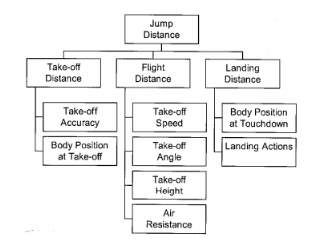
Figure 1: Long jumphierarchical technique model (Hughes and Bartlett, 2002).

Each playing position in Rugby Union comes with some responsibilities that are unique to their role, and other responsibilities that are common across all positions in the team (James et al, 2005). Hughes and Bartlett (2002) identified behavioural elements for each specific role as measures of performance. Three members of the research team (sharing knowledge of existing literature regarding this field through a combined experience of 50 years in Rugby Union and 40 in performance analysis) listed the key behaviours. They identified both common and specific KPIs for each position. Common behaviours being successful and unsuccessful actions involving; passing, tackling, carrying, tries scored and handling errors. Comparatively, a front row hooker’s throw in a line out would be classed as a specific behaviour, as this is a behaviour particular only to this player position (Hughes and Bartlett, 2002). The purpose of the Hughes and Bartlett study was not to create an extensive list of every behaviour, but more so to discover the key behaviours that contributed to an individual’s successful or unsuccessful performance. For instance, it would not be relevant to include the frequency that a hooker kicked the ball in a Rugby Union match, as this event is not very common as the responsibility of kicking does not lie with the hooker (James et al, 2005). Therefore although it can be classed as a behaviour, it is one that a) is uncommon and b) has relatively little impact on the overall success of a player or team; and therefore would not be defined not a key behaviour for that player.

2.1.1 Front Row KPIs

There are 15 starting positions in Rugby Union; certain positions can be grouped together as the individuals who carry out a similar and/or inter-linking role. One of these groups contains positions 1, 2, and 3 at the head of the team and is known as the ‘front row’. Positions 1 and 3 are the loose head and tight head props respectively, and position 2 is known as the hooker.

The loose head and tight head typically have a large stature to aid them in tackling hard, lifting players in the line-out, hitting the rucks and mauls (a ruck being where the ball is on the ground and numerous players converge, a maul being where a ball carrier is held by opposition players and players likewise converge in an attempt to gain ground), and forcing their team forward in the scrummage (BBC Sport). In addition, great importance in the modern game is now also placed on their ability to catch, time a pass for a team-mate to run into space, and run with the ball.

As well as performing all the common actions such as passing, tackling and carrying the ball, which are very important in producing a good overall performance (James et al, 2005), the front row has two main responsibilities: the line-out and the scrummage (Weston, 2007). The loose head and tight head roles lift players to catch the throw-in from the line-out and thus play integral roles in this process. Given the typical size and strength of roles 1 and 3, they also play a fundamental role in pushing the scrummage forward, thus indirectly retaining possession of the rugby ball.

In comparison, the hooker (position 2) has a slightly different role to play. As well as pushing the scrum forward, they are relied on to be an excellent ball handler who can set up intricate plays, and are hence known for their ball handling abilities. Another vastly important role of the hooker is to ensure line-out throws are successful. Given the opportunity for the opposition team to ‘steal’ the ball during a line-out, executing line-outs are often highly strategic. Each team has a variety of line-outs that they can carry out, with each strategy assigned a code word for the hooker to shout out as they begin. A successful line-out for the hooker taking the throw allows their team to retain possession and keep pressure high up the opposition’s side of the pitch. Losing possession during a line-out provides the opposition with a relief of pressure and the opportunity to counter attack. As a result, many of the pivotal roles that can influence a game fall to the hooker.

The front row is therefore often considered the key element in implementing the success of these game-changing KPIs. Hughes and White (2001) analysed the winning and losing teams in the 1999 Rugby Union World Cup and determined that teams would win more matches when their forwards were more effective in the line-out and were the better team at pushing in the scrummage – consequently retaining possession and maintaining pressure on their opposition. A test was carried out by Ortega et al, (2009) to identify any significant factors that contribute towards a winning team’s performance. Out of the 58 games of data they analysed taken from 3 years of Six Nations fixtures (an annual round robin international tournament), winning teams tended to have an efficiency rate of 90% from retaining possession from scrummaging and line-outs, and a further 94% of tackles completed successfully. However the sample size of 58 games is not very large, thus the analysis would be more compelling if the sample size was larger. Nevertheless, the test does indicate that of the factors analysed retaining possession from scrummaging and line-outs is very important.

2.2 Consistency

When reviewing the literature surrounding the project brief set by the WRU, it is immediately obvious that the topic on how consistency affects specific KPIs is a very niche area. However, there are examples of how teams who have used a minimal amount of players, and kept consistency within the team have become champions of their respective sports. For instance, the Arsenal team of 2003/04 has been voted as the best team in the Premier League’s 20 seasons (Chan, 2010). They are the only title-winning team to go the whole season unbeaten, which earnt them the sobriquet “The Invincibles”. The manager of The Invincibles, Arsene Wenger, predominately used 20 players for the whole season and used the same starting 11 players 74% of the time. Comparing this to the average number of players used in the latest 2016/17 season, which was 26, it allows the argument that consistency can play an important role towards success. There are obvious differences between football and Rugby Union i.e. less subs are available to use in football, but the concept of chemistry developing through consistently using the same players in team sports is transferrable.

Even though the literature behind relating consistency and specific KPIs to success is minimal, research did present how many authors tested for significant differences between certain KPIs and the reasons why a team wins or loses. Vaz et al (2010) attempted to identify if there were any statistics related to rugby that could discriminate between winning and losing teams. Their data was taken from the International Rugby Board (IRB), and the Southern hemisphere regional teams (S12). The study only analysed data from matches that were classed as a ‘close victory’. Vaz et al (2010) performed a cluster analysis on both of the 224 IRB games and 204 S12 games (separately analysed to preserve the disparity in each competitions style of play), allowing three different groups of games relating to the score differences to be established. 64 IRB matches and 95 S12 were classed as ‘close victories’, and were selected for further analysis, and the many variables to be tested were listed.

The statistical test, repeated measures ANOVA, was used to test the differences between the winners and losers. This test works by comparing the means of as many independent variables necessary against one or more dependent variables with many observations. It is an analysis of dependencies, as it is a test to prove an assumed relationship between these two variable groups (Statistics Solutions, 2017). In this case, the dependent variables are winners and losers, and independent variables are the range of specific KPIs. Following from this statistical test, a discriminant analysis was performed to identify 1) which independent variables are most useful in predicting the outcome of close games; 2) the equation between winning and losing teams that improved the differences in variable means and 3) the equation’s accuracies (Vaz et al, 2010). Discriminant analysis has the assumptions of independency amongst variables, equal variance/covariance across groups and multivariate normal distributions (Silva et al, 1995).

The results Vaz et al, (2010) on rugby related statistics that discriminate between winning and losing teams, found several significant differences for the S12 group. The winning teams made fewer rucks and pass movements, won more mauls and turnovers and completed fewer passes and made fewer errors. The results also showed that teams won more matches if they kicked a greater amount of their possession and made more tackles. However, it may be more appealing to assess the data using a logistic regression model instead of discriminant analysis, as it is in the process of being replaced by the regression model in more modern practices (Osborne, 2008). Instead of using the discriminant analysis, logistic regression been used in the data analysis chapters 5 and 6.

2.3 Substitutions

Due to there being little literature available on how mathematics and statistics has been used to benefit Rugby Union teams, the focus of this study has at times been aimed towards an analogous team sport, i.e. football, which has more extensive literature. As previously mentioned, there are plenty of differences between the two sports, but they have fundamental similarities relevant to the objectives of this study, namely 1) large squads with internal competition for places with emphasis often placed on matchday consistency and 2) the freedom to make a fixed number of substitutes at any point during a match.

Football managers and coaches have been utilising the statistics at their disposal for years now, and there are many cases where teams have bettered their opponents through analytical methods. AC Milan for example, put large amounts of focus on analysing statistics specific to player sustainability and the prevention of injuries (Aziza, 2010).  The team won their 7^th Champions League (considered widely to be the pinnacle of club achievement in football) trophy back in 2007, and did so fielding a starting eleven with an average age of 31. The team’s ability to keep their most experienced players fit and healthy, in the years where their age is expected to affect their fitness and ability, is a great credit to the club’s data analysts.

Once a match has started, managers have limited opportunities to affect the course of the game. As soon as the players are out on the field the responsibility of the outcome relies heavily on their shoulders.  Each team is limited to 3 substitutes per game, which can be made at any point throughout the match. The important decision of which substitution to make and when is a responsibility that the managers maintain ownership over. Substitutions in football can be a crucial factor which impact upon a team’s performance. Fatigued players can be replaced with fresh players, or tactical substitutions can be made whereby a defensive player may be brought on to protect a lead.  The tactical aspect of substitutions becomes further complicated when managers bring on players to drastically alter the formation and playing style of their own team. It is common for managers to use double substitutions, and on occasion triple substitutions may be made. Opposition managers often must react to such tactics and can be forced to play their hand earlier or later than they had planned. Substitutions are likewise as complicated in Rugby Union, however there are 7 substitutes available in a Rugby Union match, and once a player is brought off they cannot be brought back on, unless there is a blood injury which requires medical attention, or a front-row player is injured and an already substituted forward has to replace them (Feaheny, 2012) . When the stakes are high in the upper leagues of football or Rugby Union the use of substitutes is often a determining factor that managers must be keenly aware of.

The topic surrounding how to best use substitutions in football has caught the attention of many researchers who have looked at the topic from various angles, and used different mathematical techniques to assess the situation. A dynamic programming model was used by Hirotsu and Wright (2002) to find the optimal time to alter tactics, using data from the Premier League. A tactical change was related to changes in team formation as well as substitutions, and the model factored in variables such as whether a team were home or away, the time remaining, and the formation on the field. The results concerning what the difference in scores were during the game presented some interesting findings, but it was not clear how the managers would implement the proposed model positively to their team as specific times for substitutes to be used were not provided.

Another study performing an analysis on how substitutions were made in the 2004/05 La Liga season was carried out by Corral et al (2007). It was claimed that goal differential (i.e. difference in score) is a significant factor in determining what time the first substitute is made. The study backed this up with evidence supporting that teams who are losing will make a substitute earlier than teams who are winning or drawing. Also, they noted that offensive subs occurred earlier on than defensive subs. This research was very effective in analysing how La Liga utilise their substitutions, however they fail to provide managers with a specific time to make substitutes, and their data only relates to one league. Given the inherent difference in playing styles across leagues, the results may not be applicable to a league outside of La Liga.

Myers (2011), went on to look at the importance of timing for each substitution depending on certain match factors. An important point was raised in that instead of being proactive with their substitutes, managers have a tendency to be reactive. Players may be trained to last the whole 90 minutes, but as fatigue starts to become a factor their performance levels may decrease. Thus, if managers wait to substitute players once they have started to show signs of fatigue, it is most likely that the optimal time to substitute that player has already passed.

To enable their research into substitutions Myers (2011) used data, provided by ESPN Soccernet, representing 485 observations of substitutions, where 172, 155 and 158 observations came from the respective Serie A, La Liga and Premier League. They measured in the following variables; whether or not a team was home or away, the timing of each substitution and the goal differential before and after each substitution. They did not take into account what each team’s formation was, and whether or not the players was an attacker or defender. Myers (2011) produced lots of general statistics that looked at the average time teams made substitutes depending on certain variables. For instance, table 1 shows the results of a one-way ANOVA procedure, which looked at the average time each substitution is brought on depending on score positions respectively.

 

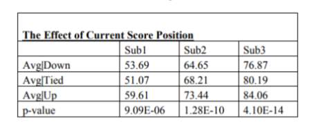
Table 1: How score positions effect substitution times (Myers, 2011).

When looking at the p-values, the results show that all three substitutions were statistically significant as each substitute produced a p-value less than 0.05, implying there was a significant difference between at least one of the mean substitution times, for each independent substitution group. Therefore, the current score of the match would significantly affect the time that a manager brings on each of their substitutes. Managers tended to make all 3 subs earlier when the team were behind or drawing, and wait longer to make a sub if the team is winning the match. This indicates that when a team is winning, a manager is more reluctant to substitute their starting players, as they do not want to interrupt a good flow of play. However, they will still be wary about player fatigue so do not want to leave it too late before using their substitutes.

The most important step to the research was to use the data mining technique of decision trees to try produce a substitution strategy that managers could benefit from. Myers (2011) developed a rule that looked at whether a team was able to improve the score state they were in once a substitution was made. A binary variable was used to demonstrate whether the score state was improved prior to a subtitute being made, the value ‘1’ indicating an improvement and ‘0’ denoting no improvement. This methodology was used to determine optimal splits in substitution time which lead to an enhanced probability of success.

The results of the decision tree came up with the proposed ‘decision rule’ that managers can utilise:

• If a team is losing, it is recommended to:
  • Make the first substitute before the 58^th minute
  • Make the second substitute before the 73^rd minute
  • Make the third substitute before the 79^th minute.
• If a team is drawing or winning, there is not specific time to make a substitute that will put the team at an advantage.

As a note, there were some conditions the rule did not apply to:

• When a substitute is forced in the first half due to an injury,
• If a match has gone into extra time, due to the score being equal after regular time, and
• If a substitute is due to a team member being red carded (presumably because a red card almost always forces a manager into a formation change).

When put to practice, teams recorded more games where their score improved if they were behind when they stuck to the substitution times of the decision rule, compared to when they did not (Myers, 2011).

2.4 Conclusion

The literature review provided insight into how analysis of consistency between front rows and optimal time for substitutions in Rugby Union is a niche area of study, with particular gaps. The review did however provide insight into the certain methodologies that can be utilised to help meet the expectations of the project brief. For instance, the use of multinomial logistic regression and a repeated measures ANOVA can be used to test whether consistency of the starting front row will have any noticeable benefits on their Key Performance Indicators. Also, the use of statistical tests that compare means of variables such as the one-way ANOVA, can be used to find significant factors that affect the times that front row substitutions are made. Finally, optimal substitution times can possibly be identified using the data mining technique of a decision tree, which should provide a specific time to bring on each front row player if there is one.

 

3 Methodology

To mathematically assess the project brief, various statistical tests were used to determine if there was enough evidence within the data to identify any significance differences between sets of variables. Different tests will be used depending on the area being analysed. For instance, it would not be suitable to use the same statistical tests to analyse if the consistency of a team benefits forward orientated KPIs, and when the optimal time to make a substitute would be as the same model might not fit both datasets. Before applying the statistical tests to the data, there are numerous assumptions that need to be satisfied to ensure the data fits the model.  The following is a summary of each statistical test to be used and their corresponding assumptions. For consistency, all tests will be performed with a significance level α = 0.05.
3.1Regression
Regression analysis is used to identify functional relationships between sets of variables, and due to its simplicity regression analysis is one of the most widely practiced statistical tools for analysing data with numerous factors (Chatterjee et al, 2015). To run a regression analysis, the data needs to be split into two sets of variables, the ‘dependent’ (or response) variable and one or more ‘independent’ (or predictor) variables. For example, analysis on how alcohol consumption is related to certain factors such as age, income and alcohol price may be an area that researchers want to investigate. The relationship between these factors can be conveyed in the form of an equation or model. In this example, the dependent variable would be alcohol consumption and the independent variables would be the various socioeconomic and demographic factors. The dependent variable is indicated by

Y, and the set of independent variables are denoted by

X1, X2, …, Xpwhere

pis the number of independent variables (Chatterjee et al, 2015). The relationship between the variables can be represented by a simple regression model:

Y=fX1, X2, …, Xp+ɛ

Where the random error defining the discrepancy in the model is denoted by ɛ. This error function is important as it takes into account that the model might not fit the data exactly. The relationship between

Yand

X1, X2, …, Xpis described by the function

fX1, X2, …, Xp. Regression models can determine how much impact each predictor variable has on the dependent variable, and can also be used to predict the outcome of the dependent variable (Cohen, 2005).

3.2 Logistic Regression

When comparing relationships between response and predictor variables, the two most frequently used models are the logistic regression model and the linear regression model. The distinguishing factor between these models is that the response variable in logistic regression is dichotomous or binary (Hosmer et al, 2013). For a response variable to be dichotomous it can only fall into one of two categories i.e. whether a team wins or loses, and is usually represented in binary form that is a 1 if the team has won, and a 0 if the team did not win. This difference between the well-known models is reflected in both the model and their corresponding assumptions.

Cox and Snell (1989) discuss some of the many proposed distribution functions used to analyse the dichotomous variables, leading them to believe there are two main reasons why the logistic distribution is chosen. It is a very flexible and easily used function, and a basis for meaningful estimates of effect are provided by its model parameters. The conditional mean of

Ygiven

x, is represented by the quantity

πx=EYx)in order to simplify the notation when the logistic distribution is used (Hosmer et al, 2013). The logistic regression model can be represented by:

πx=eβ0+ β1×1+eβ0+ β1x

The logit transformation is the transformation of

πxthat can be defined in terms of

πxas:

gx=ln⁡πx1-πx

= β0+ β1x

This is an important transformation as the function

gxhas many properties that makes the linear regression model so useful. Depending on the range of

x, the logit

gxcan range from

-∞to

+∞. It is also linear in its parameters and can be a continuous function. In logistic regression, the value of the dichotomous outcome variable given

xcan be expressed as

y = π(x) + ε(Hosmer et al, 2013). Herethe error function ɛ can be assumed to be one of two possible values:

• If

  y=1then

  ɛ=1-π(x)with probability

  π(x).

• If

  y=0then

  ɛ= -π(x)with probability

  1-πx.

Therefore, ɛ has a variance equal to

πx[1-πx]and a distribution with a mean of zero. This implies that, given the probability conditional mean of

πxthe dichotomous variable will have a binomial distribution (Hosmer et al, 2013).  The binomial logistic regression has the following assumptions:

1. The dependent variable should be measured on a dichotomous scale.
2. There must be one or more independent variables which are either measured on a continuous or categorical scale.
3. There should be independence of observations and the dependent variables categories should be mutually exclusive and exhaustive.
4. It is a requirement to have a linear relationship between the logit transformation of the response variable and any continuous predictor variables. A Box-Tidwell test is used to check for linearity.

3.2.1 Multinomial Logistic Regression

Multinomial logistic regression is a very similar case to when the outcome variable is nominal, however this form of logistic regression accounts for when there are more than two levels. For example, this test could be used to understand what type of drink people prefer based on their location in the UK, gender and their age, where the response variable would be multinomial as it has more than two categories such as water, tea, or coffee. McFadden (1974) proposed this model which is a modification on the binomial logistic regression, where the aim would be to estimate the probability of choosing any of the three drinks as well as to predict the odds of drink choice based on the covariates. The results would then be expressed in terms of odds ratios for the choice of different drinks.

Particular attention must be paid to the measurement scale when you are considering a regression model for discrete dichotomous variables with two or more responses. The assumption is made that the response variable

Yhas its categories coded as 0, 1 or 2, (in practice it is important to check that the software package being used allows a 0 code to be used, and does not have to start with 1). In this case, we would need two logit functions (Hosmer et al, 2013). For the model to be developed, the assumption is made that we have a constant term, represented by the vector

x, of length

p+1and

pcovariates, where

x0=1.

Then, the two logit functions are as follows:

g1x =ln⁡[Pr⁡Y=1xPr⁡Y=0x]

= β10+ β11×1+β12×2+…+β1pxp

=x’β1

and,

g2x =ln⁡[Pr⁡Y=2xPr⁡Y=0x]

= β20+ β21×1+β22×2+…+β2pxp

=x’β2

Following on from this, given the covariate vector the conditional probabilities of the response category are:

Pr⁡Y=0x =11+eg1x+eg2x

Pr⁡Y=1x =eg1x1+eg1x+eg2x

and

Pr⁡Y=1x =eg2x1+eg1x+eg2x

In a similar manner to the binomial logistic regression model, we let

πjx=Pr⁡(Y=j|x)  where

j=0, 1, 2(Hosmer et al, 2013). A general expression to go by for the conditional probability for the response variable that contains three categories would be:

πjx=Pr⁡Y=jx=egjx∑k=02egkx

Where the vector

β0=0and

g0x=0. The multinomial logistic regression has the following assumptions:

1. The dependent variable must be measured on a nominal level.
2. One or more independent variables that are continuous, ordinal or nominal are required.
3. There should be independence of observations and the dependent variables categories should be mutually exclusive and exhaustive.
4. There should be no multicollinearity.
5. It is required that there is a linear relationship between the logit transformation of the dependent variable and any continuous independent variables.
6. There should be no outliers.

3.3 Tests for Comparisons

A simple statistical experiment tests to see whether there are any significant differences between two means, or groups of means. Different tests are required depending on the data being analysed. If it was required to compare the means across two groups i.e. the effects of whether a team was home or away on the time a substitute is made, then a t-test would be sufficient (Andale, 2014). If the number of means required to be compared was greater than two, then using an Analysis of Variance (ANOVA) test would be more suitable to the data. There are many forms of ANOVAs that can be used, which all depends on the state the variables are in and how many are present.

 

 

3.3.1 Independent Samples t-Test

If the means of two populations need to be compared, an independent samples t-test can be an appropriate statistical test. It is also important to notice when not to use it, i.e. when observations are from a repeated measures experiment or are an ordinal level of measurement. There is a specific process that the t-test follows to enable the comparison of means. First, the two sample means

Ȳ1and

Ȳ2need to be computed using the following formulas:

Ȳ1=1n1 ∑j=1 n1Y1j

Ȳ2=1n2 ∑j=1 n2Y2j

The sample variances

s12and

s22for each group are calculated using the formulas:

s12=1n1-1 ∑j=1n1Y1j-Ȳ12

s22=1n2-1 ∑j=1n2Y2j-Ȳ22

This allows the standard error for the difference between the two samples means to be calculated by:

σȲ1-Ȳ2= s12n1+s22n2

and the degrees of freedom:

v=n1+n2-2

After all these calculations, it is possible to calculate the t-ratio using the formula:

t=Ȳ1-Ȳ2s12n1+s22n2

This is where the mean difference between groups is quantified by

Ȳ1-Ȳ2,and the mean difference within groups is quantified by

s12n1+s22n2. The assumptions for the independent samples t­-test are as follows:

1. Dependent variables should be measured on a continuous scale.
2. Independent variables consist of two categorical related groups.
3. There should be no significant outliers.
4. The differences between each pair should be approximately normally distributed, which can be checked using the Shapiro Wilk test for normality.

3.3.2 Analysis of Variance (ANOVA)

A statistical method used to analyse the dependent variable, which is measured against a number of independent variables under certain conditions is known as an Analysis of Variance (ANOVA). There are many variations of ANOVA tests, which are frequently used to compare the variance within groups against the variance between groups providing an analysis of equality between several means (Larson, 2008). ANOVAs are readily available today in the majority of statistical packages, and the task of inputting the data is very simple, hence providing easy access and accurate tests for investigators in all experimental sciences. However, it can be quite challenging for investigators to choose the appropriate ANOVA that suits their dataset, and to determine if the modelling assumptions are satisfied by the data.

There are two types of factors that distinguished by statisticians with regards to ANOVAs: ‘random factors’ and ‘fixed factors’. Random factors have a potentially infinite number of levels that represent a random sample, whereas fixed factors focus on the specific levels of interest. An investigator could repeat an experiment a number of times using identical fixed factor levels, whereas if an experiment was done using random factors it would be unlikely to have the same levels repeated (Larson, 2008). Usually, distinct populations with a unique response mean are represented by each level of fixed factors, which are called treatments if an investigator purposely modifies the levels of fixed factors. The main objective of an ANOVA testing against random factors is to make an inference about the random variation within certain populations, whereas for fixed factors it tests whether the means of the dependent variables are identical across the data’s specific levels.

3.3.2.1 One-Way ANOVA

A one-way ANOVA can be looked at as an extension on the independent samples t-test however, instead of comparing the means of two predictor variables, this statistical test allows us to simultaneously compare the means of several predictor variables (Larson, 2008). If it is required that several variables have their means compared, then this statistical test does so by testing a null hypothesis that all treatments have the same mean. A null hypothesis (sometimes represented as

H0) is used in many statistical tests, where its purpose is to determine that no statistical significances or variation between variables exist in the given set of observations. This hypothesis is assumed true, until statistically proven otherwise (Kwiatkowski et al, 1992). The alternative hypothesis (sometimes represented as

H1) would then be that at least one of the means differs from the others. Relative to the random error variance that is associated with each population, we assess whether there is sufficiently large variation among sample means that implies we should reject the null hypothesis. Thus, concluding that there exists a true difference between the population means (Larson, 2008).

The one-way ANOVA is required to satisfy the following assumptions:

1. The dependent variable must be measured at interval or ratio level.
2. There must be at least two categorical independent groups (typically it is used on data with at least 3 independent groups, but can be used on two).
3. There must be independence of observations.
4. There should be no significant outliers.
5. The dependent variable should be approximately normally distributed. This can be tested in SPSS by the Shapiro-Wilk test of normality.
6. Homogeneity of variances is required, which can be tested in SPSS by Levene’s test for homogeneity of variances.

 

3.3.2.2 Repeated Measures ANOVA

In a similar fashion to the one-way ANOVA, the repeated measures ANOVA compares the means of several predictor variables however, these variables are dependent on one another rather than being from independent groups (Laerd Statistics, 2013). Studies surrounding this statistical test investigates either the changes in mean scores under three or more different conditions, or differences in mean scores over three or more time points. The independent variables have categories called related groups (or levels), where the measurements are repeated over time and each related group is recorded as a specific point in time. For instance, if an investigation was testing to see the effects of exercise over a 6-month period on weight loss, where weight loss will be measured at 3 time periods (before, midway and after the exercise course) and the independent variable in this case would be time. Hence, for this investigation there would be three time points, each being a repeated group of the independent variable. The repeated measures ANOVA tests the related groups against the null hypothesis that there is no significant differences between the levels, in an attempt to statistically disprove the null hypothesis.

In order for the repeated measure ANOVA to process, the following assumptions need to be satisfied:

1. Dependent variables should be measures at a continuous level.
2. Independent variables should consist of at least two categorical related groups.
3. The related groups should contain no significant outliers.
4. The dependent variable in the related groups should be approximately normally distributed.
5. All combinations between related groups must have equal variances of differences, which is known as sphericity. This assumption can be tested by Mauchly’s test of sphericity in SPSS.

3.4 Decision Trees

Originating from machine learning, an efficient tool for solving classification and regression problems is a decision tree. This is a classification approach that is based on a hierarchical tree like structure or decision scheme, unlike other approaches that perform classification in a single step through the use of set features (or bands) jointly (Xu et al, 2005). The tree is composed of three types of nodes that form its structure, a root node that contains all the data, a set of internal nodes called splits and a set of terminal nodes called leaves. A binary decision is made from each node that separates one class or a set of classes from the other classes in the structure. The top-down approach is generally used, where the process is carried out by moving down the tree by creating new classes, until the leaf nodes have been reached.

Decision trees have the aim of creating a solution that is easy to understand, by splitting a complex decision into several basic decisions. In a decision tree, the dependent (response) variable is defined as the class which needs to be mapped, and the independent (predictor) variables are the different features of data (Breiman et al, 1984). There are two variations of the decision tree, a classification decision tree and a regression decision tree. A response variable that is discrete in nature would require a classification tree model. When the features carry the maximum amount of information, they are automatically chosen for classification and the computational efficiency increases as the remaining features are rejected, hence feature selection and classification are simultaneously performed. This also deals with the curse of dimensionality issue, as only a small number of features takes part in the process (Hughes, 1968). In a decision tree classifier an assumption is made that the feature and target vectors, for a sample of training data, are given. The task is to then produce a decision tree that optimises the average number of nodes in the tree, such that the training data is partitioned. This optimisation can be performed through bottom-up, hybrid or top-down approaches (Safavian and Landgrebe, 1991).

The regression decision tree approach is used when the response variable is continuous, and is built on the assumption that there is either a liner or non-linear relationship between the features (e.g. bands) and target objects (e.g. class proportions). This model is a variant of the classifier decision tree model that can be utilised to approximate class proportions from real valued functions (Xu et al, 2005). Binary recursive partitioning is an iterative process that partitions the data by splitting it, and is one aspect that the construction of the regression tree is based on. The training samples are initially used to decide the structure of the tree, and usually consist of 70% of the data although that is only a suggested percentage. Every possible binary split is then used to break the data. The algorithm chooses the split that minimises the sum of the squared deviations from the mean, where the split has partitioned the data into two separate parts. This process is applied to all the branches, and continues until the number of training samples at each node reaches a minimum size and becomes a leaf node.

Over-fitting can occur when the final structure has been reached due to the tree being constructed from a training sample, which could lead to less generalisation capability as the classification accuracy of the tree deteriorates when it is applied to data it is yet to see (Xu et al, 2005). Hence, by using a user specified cost complexity factor and a test set (usually around 30% of the data), a pruning process is generally applied. This is used to minimise the product of the total number of leaf nodes, the cost complexity factor and the sum of the response variable’s variance in the test sets. In this process, the last node to be produced is removed first.