Dissertation on Turbulent and Non-Turbulent Flows

Abstract

In this numerical study, the thin turbulent/non-turbulent interface separating the turbulent region from the irrotational fluid is studied by the means of direct numerical simulation of a developing turbulent mixing layer. A low vorticity magnitude threshold is defined to detect the position of the interface, and compute the statistical averages conditioned on the distance from the detected interface. The conditional statistical averages for vorticity are in good agreement with the results presented in past researches and studies. In addition, analysis on the comparison in considering two-dimensions and three-dimensions of the flow is conducted. The presented results show that results in both cases are nearly identical. Correlation of the statistical averages with respect to the interface and points at a distance away from it are presented. At the upper interface, which separates the high-speed flow and the turbulent region, the statistical averages for vorticity and velocity are better correlated over a longer distance than the lower interface, which separates the low-speed flow and the turbulent region. Lastly, the probability density function showed that the high-vorticity and dissipation worm-like structures in the turbulent region tend towards the upper interface.

Click to expand Table of Contents

Table of Contents

Introduction

Project Objectives

Thesis Outline

Literature Review

Structure of a Turbulent/Non-Turbulent Interface

Detection of the Turbulent/Non-Turbulent Interface

Scaling of the Turbulent/Non-Turbulent Interface

Other Types of Interfacial Layers

Passive Scalars in Interfacial Layers

Interfacial Layer between Laminar Boundary Layers and Free Stream Turbulence

Shear-Free Interfaces with Stratification

Flows with External Turbulence and Internal Forcing

Challenges in Turbulence Modelling of Interfacial Layers

Procedure

Flow Parameters and Numerical Modelling

Model Validation

Detection of the Turbulent/Non-Turbulent Interface

Statistical Averages with Respect to the Turbulent/Non-Turbulent Interface

Results and Analysis

Evolution of Mean Position of the Interface

Statistical Averages (2D) Normal to the Interface (Streamwise)

Statistical Averages (2D) Normal to the Interface (Spanwise)

Statistical Averages (3D) Normal to the Interface

Correlation of Statistical Averages

Positions of Large Vorticity and Dissipation Structures

Conclusion

Table of Figures

Figure 1 Detailed Schematics of a Turbulent flow (2)

Figure 2 Vortical Flow Fraction as Function of Vorticity Magnitude (2)

Figure 3 Mean Conditional Tangential Vorticity as a function of distance from the interface (10)

Figure 4 Illustration of the Turbulent/Non-Turbulent Interface (16)

Figure 5 Influence of Richardson Number on the Interface (2)

Figure 6 Averaged Velocity Profile over Three Time-Steps as a function of y/h

Figure 7 Vortical Flow Fraction over a Range of Vorticity Magnitude from 0 to 5

Figure 8 Vortical Flow Fraction over a Range of Vorticity Magnitude from 0 to 1

Figure 9 Contours of the Vorticity Magnitude with the Vorticity Threshold at 0.01

Figure 10 Contours of the Vorticity Magnitude with the Vorticity Threshold at 0.008(left) and 0.012(right)

Figure 11 Mean Profile across the T/NT Interface

Figure 12 Conditional Average of Vorticity Magnitude by Antonio Attili et al. (1)

Figure 13 Comparison in Vorticity Jumps at Different Threshold Levels

Figure 14 Isosurfaces of Interface at

ω=0.11(right) and

ω=0.21(left)

Figure 15 Statistical Averages of the Crosswise Position of the Interface along Streamwise(Left) and Spanwise(Right) Direction

Figure 16 Normal Vectors on a Circle

Figure 17 Statistical Averages of Vorticity

Figure 18 Statistical Averages of Turbulence Kinetic Energy Dissipation

Figure 19 Statistical Averages of Vorticity

Figure 20 Statistical Averages of Turbulence Kinetic Energy Dissipation

Figure 21 Statistical Averages of Vorticity about Angle

Figure 22 Statistical Averages of Vorticity about Angle

Figure 23 Statistical Averages of Turbulence Kinetic Energy Dissipation about Angle

Figure 24 Statistical Averages of Turbulence Kinetic Energy Dissipation about Angle

Figure 25 Statistical Averages of Velocity about Angle

Figure 26 Statistical Averages of Velocity about Angle

Figure 27 Statistical Correlation Averages of Velocity about Angle

Figure 28 Statistical Correlation Averages of Vorticity about Angle

Figure 29 Statistical Correlation Averages of Velocity about Angle

Figure 30 Statistical Correlation Averages of Velocity about Angle

Figure 31 Comparison of Correlation with respect to Different Positions

Figure 32 Probability Density Functions of the Distances of High Vorticity and Dissipation Structures

Introduction

In turbulent flows, such as wakes and mixing layer, the turbulent and non-turbulent (irrotational) regions are separated distinctly by visible interfacial layers (1). These layers are essential and critical in turbulent combustion and cloud mixing as they affect entrainment and mixing (1).

An interfacial layer is defined as a thin region with finite thickness that separates either regions of different turbulence intensities or turbulent flow and non-turbulent region (2). It is usually identified by the vorticity or scalar concentration gradients from the region. The existence of laminar superlayer, as shown in Figure 1, was first proposed by Corrsin & Kistler in 1955 from the first examination of interfacial process which transpires adjacent to a free shear layer and that separates turbulent from non-turbulent regions (3).

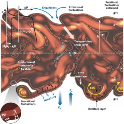
Figure 1 Detailed Schematics of a Turbulent flow (2)

Reynolds argued the impossibility of a maximum vorticity magnitude across the interfacial layer (4), however, an approximately continuous interfacial layer, with a peak in vorticity and a thickness corresponding to Taylor microscale was discovered by Bisset et al. (5) and Westerweel et al. (6) through numerical simulations and experiments. Despite similar conclusions on the presence of interfacial layers, numerical simulations and experimental results presented different findings on microscale vortices. Direct numerical simulations (DNS) showed the existence of elongated microscale vortices within the interfacial layers (7,8), while experimental studies observed vortices moving at a characteristic microscale speed relative to the large-scale flow, this indicated the vortices have no direct relation to the behaviour of the movement in the interfacial layer (9).

This thin interfacial layer, separating the turbulent and irrotational regions, is discovered to consist of two layers (2), the viscous superlayer and the turbulent sublayer. The former introduces vorticity to the irrotational flow through viscous diffusion and its thickness is found to be of the order of Kolmogorov microscale, whereas the latter is responsible for the vorticity variations from the viscous superlayer to the core of the turbulent region and its thickness is comparable to the Taylor microscale (1,2).

One common technique employed to detect interfacial layers incorporates the use of a low vorticity magnitude threshold, where regions with vorticity below the threshold are deemed as irrotational. Bisset et al. pioneered the approach of using conditional statistics and analysis of interfacial layers had benefited much from it (2). Using classical statistics, the large-scale intermittency of the flow smoothened the mean profiles from the turbulent and irrotational region, whereas conditioned statistics provided much steep gradients at the interfacial layers instead (2).

Project Objectives

Previous studies and investigations involved specifying a vorticity magnitude threshold to define the interfacial layer of the turbulent flow, then deriving the conditional statistics from a distance away from the interfacial layer normal to the flow direction. Results had shown that across an interfacial layer, the conditional statistics displayed a jump in magnitude, like a step function. However, these analyses are limited to the statistics normal to the flow direction and the results involves only two-dimensions (streamwise/crosswise plane) of the turbulent flow.

Thus, with the given field of data in three different time-steps of a spatially developing mixing layer, this numerical study will explore new methodology by creating new local coordinate system normal to the interfacial layer and investigate the conditional statistics along a line normal to the specific point of the interfacial layer in both two- and three-dimensions of the turbulent flow.

This numerical study will be done in different stages:

1. Methodology validation by acquiring similar results as shown in previous investigations using conditional statistics
2. Examination(2D) of the conditional statistics across the local coordinate system normal to the interfacial layer in the streamwise/crosswise plane and spanwise/crosswise plane
3. Examination(3D) of the conditional statistics across the local coordinate system normal to the interfacial layer
4. Examination of the correlation of the statistics with respect to different points near the interfacial layer
5. Study on the position of the high magnitude structures in the turbulent region

Thesis Outline

The organisation of the thesis is as follows. The “Literature Review” section will present the current state of art on interfacial layer of turbulent flows, covering the structure and scaling of interfacial layers, detection and identification of interfacial layers in a flow and lastly, different types of interfacial layers and their respective dynamics. “Procedure” section presents flow configuration, parameters, the proposed methodology used in this numerical study and the results of the model validation in the detection of the turbulent/non-turbulent layer, in which the statistical averages of the vorticity across the interfacial will also be presented. Lastly, the main results of this numerical study will be presented and discussed in the “Results and Analysis” section.

Literature Review

In the study of interfacial layer, the velocity fluctuations can originate from two important velocities as shown in Figure 1:

1) Boundary Velocity, Eb, the velocity at which the interface moves outwards as the turbulent flow expands with time and distance and,

2) Entrainment Velocity, Ev, being affected by various aspects of the velocity fields, they vary in magnitude and directions towards the interface for different turbulent flows (2). Fluid elements in the irrotational regions outside the interface may acquire vorticity from the turbulent regions in two ways: either 1) locally at selected areas where there are large fluctuations due to engulfment, an inviscid component of the outward growth, caused by the consumption of external fluid, or 2) along the interface through nibbling, a partially viscous process that results in an outward growth from the irregular eddy-motions near the interface  (10). These processes then associate the two velocities happening at the interface together (11).

Structure of a Turbulent/Non-Turbulent Interface

In wakes and boundary layers, there are intermittent zones between the turbulent regions and adjacent regions with no turbulence intensity (5). This interfacial layer, known as the turbulent/non-turbulent (T/NT) interface, is the simplest and extreme case of an interfacial layer between two regions of different intensity with zero at one side (2). It is important to note the difference between the viscous superlayer discovered by Corrsin and Kristler (3) and the T/NT interface. The latter is a very thin layer of fluid with zero thickness where major changes across the irrotational fluid and fully turbulent flow occur, whereas the former forms the outer boundary of the T/NT interface (5).

In Figure 1, the interfacial layer is structured with two adjacent layers: the viscous superlayer, denoted with

δv, and turbulent sublayer, denoted with

δw. The viscous superlayer exists to control the diffusion process which the irrotational region acquires vorticity, however, there has been no observation or report on the existence of such layer (10). The turbulent sublayer must match the vorticity from the turbulent region to the vorticity in the viscous superlayer (2). Thus, the T/NT interface is often referred as the turbulent sublayer with a finite thickness.

Detection of the Turbulent/Non-Turbulent Interface

In a fully developed turbulent flow, the vorticity magnitude of each fluid elements in the turbulent flow is expected to be non-zero whereas any fluid elements outside the turbulent flow are considered irrotational (zero vorticity magnitude). Hence, a simplest and straightforward approach will be to distinguish the regions with zero and non-zero vorticity magnitude to determine the position of the interface. However, the presence of numerical and experimental noises negates the feasibility of the simple approach (2,5). In experiments, the combination of free-stream turbulence and instrument noise result in a non-zero vorticity in the non-turbulent region, and similarly, background noise in numerical simulations has the same effect to the non-turbulent regions [1].

There have been several methodologies and techniques deployed to reduce the effect of noises on the irrotational region to detect the position of the T/NT interface in the turbulent flow. One technique involves a low-vorticity magnitude threshold, below which flow regions can be viewed as irrotational [2]. The selection of the threshold relies on the observation of the magnitude range in which the statistics in the interface is weakly dependent on the threshold value. Figure 2 illustrated the relationship between the vortical flow fraction and the normalised vorticity magnitude (vorticity magnitude normalised by the root-mean-square velocity and integral length scale,

ω̃=ωL/u(H)) [2]. The vortical flow fraction was observed to experience a sharp drop, followed by a plateau then lastly, a very slow descent with the increase in vorticity magnitude. Hence, it can be concluded that any magnitude threshold within the observed plateau can be applied to detect the position of the interface.

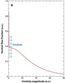
Figure 2 Vortical Flow Fraction as Function of Vorticity Magnitude (2)

In a numerically simulated wake, it was found that the contour at

Cω=0.7U0/b(with

U0 and breferring to the mean velocity of the wake and the width across both sides of the wake respectively) best depicted the vorticity in the wake (5). Contours between the stated level spread into the free-stream in a disorganized manner, whereas contours above the level outline many small low-vorticity region in the wake interior (5). It is important to note that the detected surface approximates the outer boundary of the T/NT interface, and it is impossible to define the thickness of an interface except in a conditionally averaged sense (5). The use of conditional statistics relative to the interface was pioneered by Bisset et al. (2) and the approach consists of the following steps: 1) detect the interface position using a vorticity threshold mentioned above, 2) define an interface envelope with coordinate

yi, 3) define a new local coordinate system on the interface and compute the statistics in the new local coordinate system (5).

Conditionally averaged measurements relative to the interface depicted a jump in the tangential vorticity component as the fluid element moves into the interface as shown in Figure 3. According to Bisset et al. and Westerweel et al., the mean profiles can be approximated as a step function with a linear gradient (5,10).

Other than the above approaches chosen for this numerical study, there are other methodologies used to define the T/NT interface. They consist of analysing 1) the vorticity probability density functions at points through the edge of the turbulent flow to observe for a change of shape (12), 2) a passive scalar field of very high Schmidt number (6) and 3) the turbulent kinetic energy (13). However, the observed change in turbulent kinetic energy across a shear free layer is not as drastic as the change in vorticity magnitude.

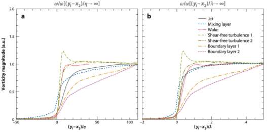
Figure 3 Mean Conditional Tangential Vorticity as a function of distance from the interface (10)

Scaling of the Turbulent/Non-Turbulent Interface

The thickness of the viscous superlayer,

δv, was estimated to be of the order of Kolmogorov microscale,

η=υ3ε14, where υ: kinematic viscosity  ε: turbulent kinetic energy. Kolmogorov microscale is known as the smallest scale in turbulent flow, where viscosity dominates and turbulent kinetic energy is dissipated into heat energy. This scaling had been validated in experiments in the turbulent front generated by an oscillating grid (13) and a turbulent round jet (14). However, the features of this layer were not directly captured. Similarly, other studies had highlighted that the important viscous effects near the edge of the T/NT interface can only be observed at very fine resolution no larger than

η(15).

As mentioned above, the turbulent sublayer is often referred as the T/NT interface. In several flows, changes in vorticity magnitude and scalar gradients are observed across this layer, thus the thickness of the turbulent sublayer (T/NT interface) can be assumed as the thickness in which the sudden jump in vorticity and scalar gradients were observed. In present flows, the thickness of the turbulent sublayer,

δw, is approximately

0.06b-0.08b, which is comparable to Taylor microscale,

λ(5). The scaling of turbulent layer is related to the geometry of the T/NT interface because it is defined by the regions of vorticity in the form of vortex tubes, where the radius of the largest vortices is approximately similar to the turbulent sublayer thickness (16).

As shown in Figure 4, the T/NT interface has an extremely complex geometry, influenced by the type of flow and the turbulence intensity. Despite the exhaustive studies on T/NT interfaces, there are persisting questions on the geometry of T/NT interfaces in free shear flows. It is unclear which statistics, for example the shape of the probability density functions, are universal and which depend on the flow type, initial conditions etc. (2). Some features are flow dependent as the large convolutions are outlines of the large-scale vortices under the interface, while small-scale features of the interface may be universal depending on the scale (5).

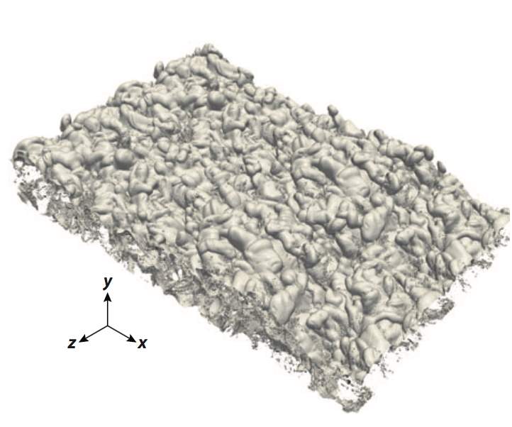
Figure 4 Illustration of the Turbulent/Non-Turbulent Interface (16)

Other Types of Interfacial Layers

Passive Scalars in Interfacial Layers

In many turbulent flows, scalars are introduced either from a point source in an inhomogeneous layer or as area fluxes at the boundaries of the turbulent region (17,18). It is extremely important to understand the dynamics of the interface and scalar dissipation. Experimental and numerical results had exhibited a jump in the scalar gradient similar to the mean velocity, with a thickness thinner than the vorticity field (10,15). As the mechanisms governing the passive scalar in the T/NT interface inherit much steeper gradients than the mechanism for the velocity field, the dynamics of passive scalars appear to be more challenging (15).

Interfacial Layer between Laminar Boundary Layers and Free Stream Turbulence

Resulting from the no-slip condition and blocking, boundary layers generate significant shear, affecting the ability of disturbances above and outside the boundary layers to penetrate the interface. Inviscid shear sheltering dominates when the fluctuations are at approximately same velocity as the external flow (19). The fluctuating shear related to blocking results in instability in laminar boundary layers, and when the Reynolds number is high enough, they will transit to turbulent boundary layers. Idealized linear calculations have shown that shear dominates the blocking effect on the wall and at high Reynolds number, the disturbances decay exponentially at the edge whereas at low Reynolds number, oscillatory disturbances penetrate the wall (20).

Shear-Free Interfaces with Stratification

Stable stratification influences the amplitude of interfacial fluctuations which can lead to trapping on one side of the layers. Richardson Number,

Ri= ∆ρgL/ρuH2, is used to characterise the properties of the flow at a sharp step stratification with turbulent region of density,

ρ+∆ρ, and non-turbulent region with density,

ρ(2). Figure 7 illustrates the influence of Richardson number on the morphology of the interface. In the figure, the turbulent region is denoted by

R(-), non-turbulent region by

R(+)and the colour of the contours describes the local density of the fluid. At low Ri, the interface is completely dominated by engulfment. Increasing Ri results in eddy impingement on the interface and mixing by Kelvin-Holmholtz instabilities inducing eddies (21). When Ri reaches beyond 40, entrainment tyrannized by breaking interfacial waves.

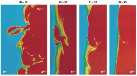
Figure 5 Influence of Richardson Number on the Interface (2)

Flows with External Turbulence and Internal Forcing

Complex mechanisms arise when there is turbulent flow outside the shear layer of interest or the presence of fluctuating body forces, increasing the internal turbulence (22,23). These can occur in the interior of the turbulent flows, in jet discharges (22), at the tops of canopies or buildings (24), or at the top of the viscous sublayer near a fixed wall (25). In these occurrences, the interface breaks down, either when the turbulence in the high-intensity regions decays or when heat is induced to the high intensity region (2).

Challenges in Turbulence Modelling of Interfacial Layers

For one-point closures, both turbulence kinetic energy,

k=u2/2and viscous dissipation rate,

εtend to zero in irrotational region. Therefore, in Eulerian one-point statistics, dissipation length scale,

lε=k32/εand eddy viscosity

υe=k2/εbecome ill-defined, creating numerical problems in the Reynold-Averaged Navier-Stokes (RANS) computation (26). A simple solution can be producing the correct mean profiles with RANS, or the correct interface, or a compromise of both but one aspect of flow physics will be unrealistic (5). A classic solution involves using a constant finite eddy viscosity at the outer edge of shear layers that decreases to a smaller value of a background eddy viscosity inside the irrotational region (27).

Statistical models based on

kor

εare widely used despite the uncertainty in the solutions due the dependence of numerical approximations (5). The models are unable to differentiate the dynamics at both side of the T/NT interface, thus one way to examine the limitations is to compare the spatial distribution relative to the interface using conditional sampling to the conventional distribution in the fixed coordinates (5). Results revealed that the statistical models do not represent the dominant dynamics of the interface completely. Diffusive modelling describes the momentum or scalars transfer towards the interface, but the processes at the interface are not well explained (5). Investigations showed that with appropriately chosen coefficients, such statistical models might reproduce the properties of the T/NT interface (5,6,26). But the models cannot represent the statistics of fluctuations or the mean field where the gradients of scalars are present in the external quiescent fluid (28).

For subgrid-scale models, it is shown that motion near the T/NT interface are not in equilibrium and consist an important fraction of the total kinetic energy of the flow (29). This phenomenon violates the assumptions applied in Large-Eddy Simulations (LES) approaches, and many subgrid-scale models are unable to handle it. The local dynamics at the T/NT interface at scales smaller than the grid size are not well represented in LES, contributing to the errors in calculations and estimations at the T/NT interfaces. Moreover, subgrid-scale modelling of a passive scalar near the T/NT interface may be more challenging and complex than for velocity field because of the small scales for mixing (2). More importantly, very little information is available on subgrid-scale modelling on this context.

Procedure

Flow Parameters and Numerical Modelling

In this numerical analysis, a flow configuration of two independent streams of velocity

u1and

u2flowing on the opposite sides of a rectangular plate as shown in Figure 6, with a constant thickness of

yh=0.9627, stretched across the spanwise direction, was investigated. The Reynolds number,

Re, dependent on the velocity scale

û= (u̅max+u̅min)/2and the Kolmogorov microscale expressed in terms of

his 1000 and the velocity ratio,

u1/u2= 0.5, where

u1is the low-speed flow at the bottom of the plate and

u2is the high-speed flow at the top of the plate.

As this analysis focused on the behaviour of the flow across the T/NT interface, only a small portion of the domain,

nx×ny×nz= (301×507×256), will be used for calculation and analysis. This is done to ensure that the studied domain is a fully developed turbulent flow and to save computation time.

Model Validation

Detection of the Turbulent/Non-Turbulent Interface

With the data on the velocity field of the flow at three individual time-steps and the C++ code provided to perform the necessary calculations, the mean profile of the streamwise-component of the velocity, averaged across streamwise and spanwise directions, at each time-step and the average turbulent kinetic energy dissipation rate,

<ε>and the root-mean-square (RMS) velocity of the homogeneous turbulent flow at different vorticity thresholds were calculated.

Knowing that the Kolmogorov microscale is

η=υ3ε14, the kinematic viscosity was calculated and expressed in terms of h using the relationship of Reynolds number, kinematic viscosity and the velocity scale. From the results shown in Figure 6, the velocity scale,

u̅, turned out to be

0.9443, resulting in the kinematic viscosity as

9.4434 × 10-4h. The average turbulent kinetic energy dissipation rate

<ε> =2υ, where

Sij=12(∂ui∂xj+∂uj∂xi)is the fluctuating rate of strain tensor, was calculated individually at each time-step before averaging over the three time-steps Together with

<ε> =3.5546 × 10-4, the Kolomogorov microscale,

η, was calculated to be

0.03942h.

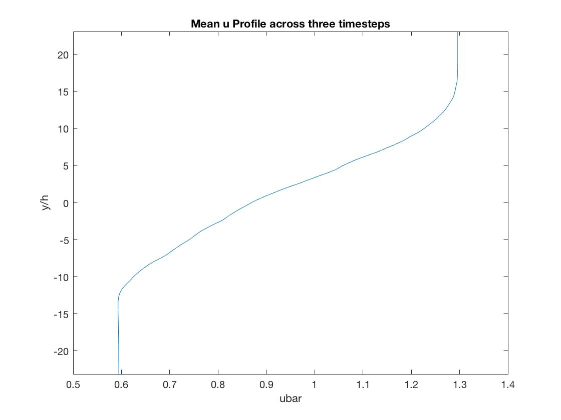
Figure 6 Averaged Velocity Profile over Three Time-Steps as a function of y/h

Adopting the low-vorticity magnitude threshold method (2) to determine the vorticity threshold,

ω̃=ωL/u(H), a range of vorticity magnitude from 0 to 5 at an interval of 0.01 was normalised by the RMS velocity of 0.9499 and Kolmogorov microscale of 0.0392. The vortical flow fraction was plotted accordingly as a function of the normalised vorticity threshold as shown in Figure 7, these results are then compared to the results shown by Carlos et al. in Figure 2 (2).

With a wide range of vorticity magnitude, the results portrayed a steep drop at the start, followed by a subtle descent in vortical flow fraction as the vorticity threshold increases. Compared to the findings by Carlos et al. (2), a plateau was expected immediately after the sharp drop in vortical flow fraction. However, in this case, no plateau was observed. Assuming that the plateau is expected to appear immediately after the steep drop, the vortical flow fraction should fall within 0.6 and 0.7 in this case. Hence, the range was reduced so that the vortical flow fraction at 0.5 to 0.8 can be better visualised.

After reducing the range of vorticity magnitude to be simulated to 0 to 1 at an interval of 0.01, a much gradual decrease in vortical flow fraction was observed after the steep drop at the start. Despite the absence of a plateau in this range of vortical magnitude, it could be seen that at

ω̃=0.01, the flow at both

t=11and

t=900had the same vortical flow fraction at 0.7 while the vortical flow fraction at

t=101was approximately between 0.65 and 0.7. Thus, the vorticity magnitude threshold used in this numerical study will be 0.01.

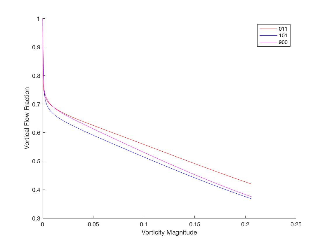
Figure 7 Vortical Flow Fraction over a Range of Vorticity Magnitude from 0 to 5

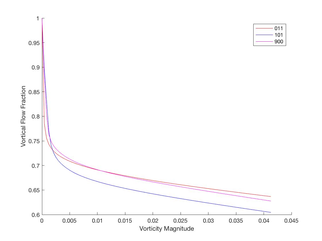
Figure 8 Vortical Flow Fraction over a Range of Vorticity Magnitude from 0 to 1

To ensure the T/NT interface is independent of the vorticity magnitude threshold, 3D flow visualisation was performed using Paraview 5.4.0-RC3 combining all three time-steps for simplicity and better visualization. Contours of the interface at

ω̃=0.01were plotted along with contours at various vorticity magnitude thresholds.

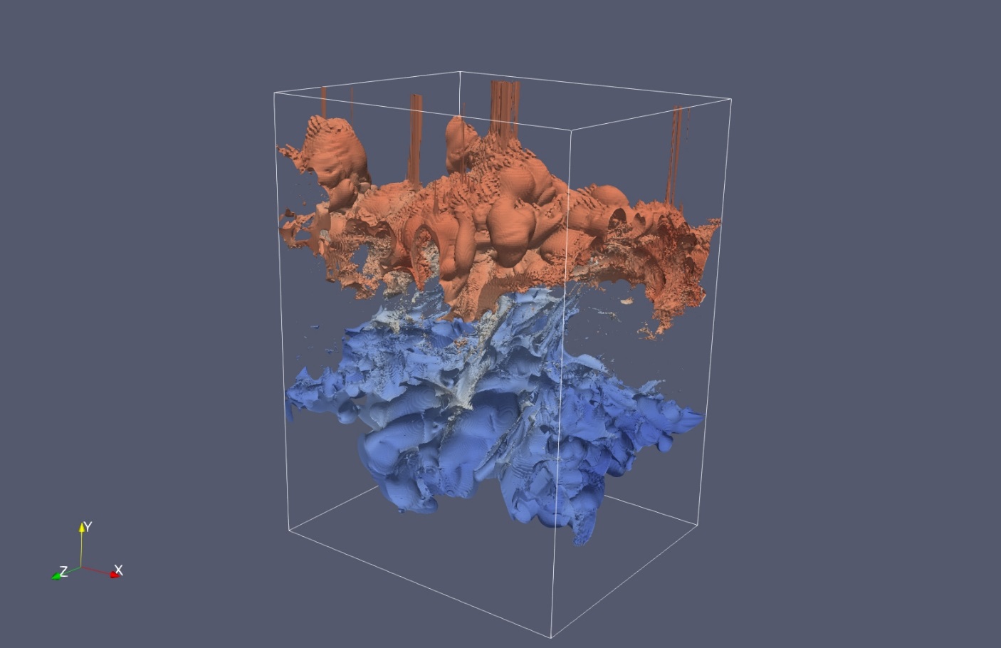
Figure 9 Contours of the Vorticity Magnitude with the Vorticity Threshold at 0.01

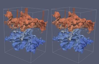
Figure 10 Contours of the Vorticity Magnitude with the Vorticity Threshold at 0.008(left) and 0.012(right)

In Figure 9, when the threshold was set at

ω̃=0.01, the irrotational and turbulent regions were defined clearly and the T/NT interface could be easily identified where the red isosurface (upper interface) meets the high-speed flow and the blue isosurface (lower interface) meets the low-speed flow. The contour plotted at

ω̃=0.01resembles much like the T/NT interface illustrated in Figure 4. The interface defined by varying the threshold

ω̃=0.008and

ω̃=0.012also produced near similar results, distinguishing the turbulent and irrotational regions clearly. From these comparisons, it can be concluded that the T/NT interface is independent of vorticity threshold at approximately 0.01.

Statistical Averages with Respect to the Turbulent/Non-Turbulent Interface

To testify that the identified interface behaves similarly as what were discovered in previous works, the vorticity across the interface will be used for validation, utilizing the conditional statistics approach by Bisset et al. (5)and defining a distance from the interface along the direction normal to the flow direction. As shown in Figure 9, the turbulent flow inherited several thicknesses and consists of bubbles of various sizes along the streamwise direction. Along the streamwise and spanwise direction, the lines parallel to the crosswise direction at some nodes passed through several irrotational regions, experiencing multiple jumps in vorticity. Thus, to eliminate any form of turbulent bubble or entrainment, a condition in which, the data was only acceptable if the vorticity only experienced a jump instead of multiple jumps, was enforced onto the selection of data to warrant the flow at the node moves from irrotational region to turbulent region once. Vorticity statistics parallel to the crosswise direction, are computed, conditioned on the distance from the interface ranging from

yi-y=-2to

yi-y=2, where

yiis the position of the interface, by averaging along both streamwise and spanwise directions and in time. The flow is turbulent when

yi-y>0, whereas

yi-y<0denotes the irrotational region of the flow.

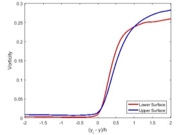
Figure 11 Mean Profile across the T/NT Interface

In Figure 11, the mean profiles across both sides of the T/NT interface experienced a sharp climb in vorticity with approximately similar gradients while moving into the interface from the irrotational region. However, as the velocity stream at the upper surface was moving faster than the velocity stream at the lower surface, two jumps of different magnitude from the two surface of the T/NT interface was observed at the interface position. It is important to note that both T/NT interfaces are two morphologically different entities. Comparing these results to the investigations by Antonio Attili et al. (1), these results resembled much closer to the conditional average of vorticity magnitude for the low-speed (solid line) and high-speed (dashed line) streams in Figure 12.

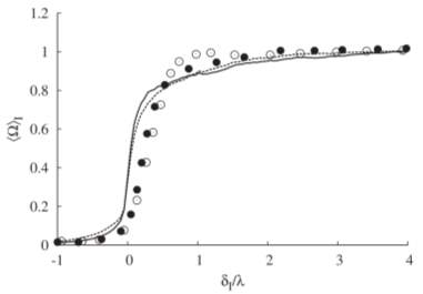
Figure 12 Conditional Average of Vorticity Magnitude by Antonio Attili et al. (1)

A comparison in vorticity jumps was done to survey its behaviour in relation to the threshold level. Figure 13 depicted the vorticity jumps across both interfaces at different threshold levels. As the vorticity threshold increases, the vorticity in the irrotational region naturally increases. From the results, a difference in vorticity in the irrotational region was observed. At both top and bottom of the T/NT interface, overshoots were observed in the vorticity at both

ω̃=0.11and

ω̃=0.21, behaving in a dissimilar fashion as when the threshold was at

ω̃=0.01, and the magnitude of the overshoots was observed to be approximately twice the magnitude of the vorticity jump when

ω̃=0.01. From the observations of the comparison in vorticity jumps over a certain threshold level, the vorticity jump at the interface at both

ω̃=0.11and

ω̃=0.21presented much steeper gradients, in much agreement with the results in the previous analyses. However, the results presented by Antonio Attili et al. (1) showed that the vorticity settled down after the jump without any presence of overshoot. And from the 3D contours of the interface, threshold levels of

ω̃=0.11and

ω̃=0.21outline about 80% of the turbulent flow (shown in Figure 14), which violates the characteristics of a T/NT interface.

With the current methodology adopted in this numerical study, fitting statistical averaged profiles were produced and displayed behaviours like the results of previous analyses. The resemblance in behaviours demonstrates a certain level of agreement on the flow physics near the T/NT interface. It is evident that the difference is relatively insignificant and the results will not be greatly affected. Hence, this methodology will be used in this numerical study to observe the behaviour of the flow with respect to a new local coordinate system normal to the interface.

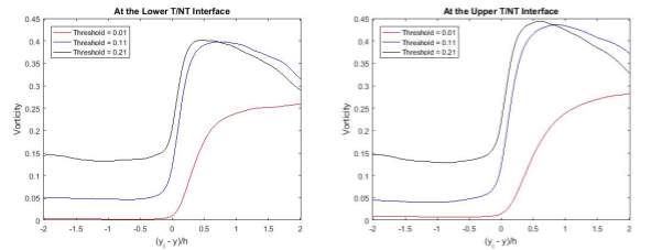
Figure 13 Comparison in Vorticity Jumps at Different Threshold Levels

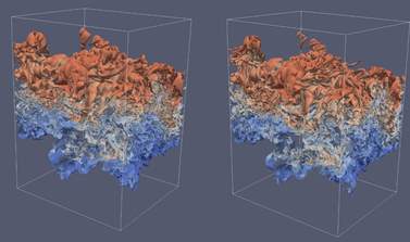
Figure 14 Isosurfaces of Interface at

ω̃=0.11(right) and

ω̃=0.21 (left)

Results and Analysis

Evolution of Mean Position of the Interface

Statistical analyses were done on the position of the interface in the crosswise direction, the results are shown in Figure 15 (red for upper interface and blue for lower interface). The mean position is characterised with a linear evolution, with the assumption of self-similarity for the mixing layer (1). Hence, with the statistical averaged crosswise position of the interface in the streamwise and spanwise direction, best linear-fit lines were plotted at the top and bottom interface to observe the mean position evolution along both directions. As expected, the position of the lower and upper interfaces move away from the centre of the flow,

yh=0, along the streamwise direction, expanding the size of the turbulent region. In the spanwise direction, the position of the lower interface shifts towards the centre of the flow, while the position of the upper interface shifts away from the centre of the flow instead. This observation showed that the flow does not increase its size in the spanwise direction, unlike in the streamwise direction.

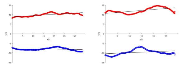
Figure 15 Statistical Averages of the Crosswise Position of the Interface along Streamwise(Left) and Spanwise(Right) Direction

In comparison of the mean position in both directions, one notable observation made is the mean position in the spanwise direction presented greater deviation from the linear fit as compared to the mean position in the streamwise direction. In the region at the middle of the flow in the spanwise direction,

zh=10-15, the thickness of the turbulent region appeared to be thinner than the thickness nearer to the boundary of the flow.

Statistical Averages (2D) Normal to the Interface (Streamwise)

To examine the statistical averages normal to the interface, two-dimensional vectors with component

xy and angle

ϕϑ with respect to the global coordinate axes, normal to the interface were created at each point of the interface. Data at distance from the interface ranging from

yi-y=-2to

yi-y=2were extracted and interpolated accordingly using the nearest nodes of the computational domain. Statistical averages on vorticity and turbulent kinetic energy dissipation were computed and analysed. Likewise, the condition of only one vorticity jump to ensure there is only one transition from irrotational to turbulent region was applied.

Ensuring that the normal vector is created correctly, the methodology is applied onto a simple geometry, in this case, a circle. As shown in Figure 16, the lines plotted from the circumference of circle are the normal vector to the circle at each degree, validating the methodology.

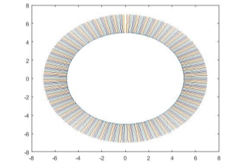
Figure 16 Normal Vectors on a Circle

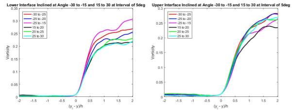
Figure 17 Statistical Averages of Vorticity

One unique characteristic of the T/NT interface is the orientation at each point is different spatially and temporally. Therefore, to ensure the accuracy of the results and sufficient data will be captured, a range of angle in the interval of 5 degrees was used. When the normal is oriented at a negative (positive) angle, the interface is leaning towards the upstream (downstream) at the upper interface, and vice versa for the lower interface. From the results shown in Figure 17, at both interfaces, the vorticity experienced a jump in magnitude at approximately similar gradient. However, at the lower interface, at different ranges of orientation of the normal vector, after the jump, the vorticity at different ranges settled at different magnitude from 0.2 to 0.32, whereby at the upper interface, the vorticity at different range of orientation settled at a much closer range of magnitude except for the normal oriented from 15 to 20 degree.

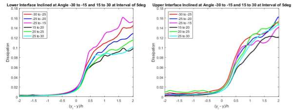
Figure 18 Statistical Averages of Turbulence Kinetic Energy Dissipation

Figure 18 displayed the statistical averages of the turbulence kinetic energy dissipation in the streamwise-crosswise plane. The dissipation relative to the interface is characterised by a jump, followed by a rather smooth increment in magnitude. Like the statistical averages on vorticity, the dissipation hit a larger range of magnitude after the increment at the lower interface as compared to that at the upper interface. From past studies and experimental reports, it was reported that the dissipation will increase slowly and smoothly to the value at the centre of the flow after the jump [3]. However, the results presented fluctuations after the jump at both interface. This could be due to the lack of information in the temporal development of the flow.

Statistical Averages (2D) Normal to the Interface (Spanwise)

Likewise, in the spanwise-crosswise plane, two-dimensional vectors with component

yzand angle

ϑψwith respect to the global coordinate axes, normal to the interface were created at each point of the interface. The method to compute the statistical averages in the streamwise-crosswise plane was used in the case of spanwise-crosswise plane. The results on the statistical average of vorticity were shown in Figure 19 for the lower and upper interface respectively.

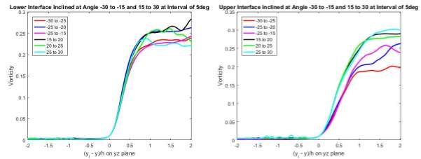
Figure 19 Statistical Averages of Vorticity

One key observation made was the vorticity at the lower interface settled at a smaller range of magnitude, as compared to at the streamwise-crosswise plane (Figure 17), and lesser fluctuation was observed after the jump showing that the vorticity settled earlier in the spanwise-crosswise plane.

The statistical averages at the upper interface in the spanwise-crosswise plane presented a slightly different result as that in the streamwise-crosswise plane (Figure 17). The gradients of the vorticity jump when the normal is oriented at a negative angle is gentler than the gradients when the normal is positive-oriented. Also, the latter settled and tended towards a unified value whereas the former settled at range of magnitude below the settling magnitude of the latter.

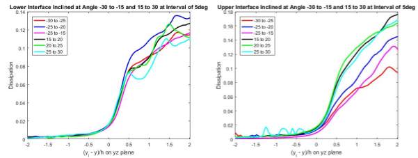
Figure 20 Statistical Averages of Turbulence Kinetic Energy Dissipation

Figure 20 illustrated the statistical averages of the turbulence kinetic energy dissipation in the spanwise-crosswise plane. Likewise, the dissipation at both interfaces behaved with a jump at the interface, followed by a slow increment moving into the turbulent region. At the lower interface, greater fluctuations were observed after the jump instead of a smooth increment. At the upper interface, when the normal is positive-oriented, a steep increase followed by a rather fast increment while the turbulence kinetic energy dissipations with negative-oriented normal started rising at the interface and the increment appeared to be constant, moving into the turbulent region.

As mentioned above, each position of the T/NT interface is not identical spatially and temporally, indicating that the interface is facing many different directions at each point of time. From the results from the model validation and statistical averages in both planes, the difference in magnitude of vorticity jump caused by the orientation of surface is trivial, especially for the statistical averages of the streamwise-crosswise plane and spanwise-crosswise plane. However, the surface orientation has a considerable effect on the turbulence kinetic energy dissipation. Significant differences in behaviour of the dissipation statistical averages were observed.

Statistical Averages (3D) Normal to the Interface

Using the same methodology to create the normal vector, three-dimensional vectors with component

xyzand angle

ϕϑψwith respect to the global coordinate axes, normal to the three-dimensional interface surface were created at each point of the interface by associating the normal in the respective planes at each point together. To make a reasonable comparison with results in the 2D cases, statistical averages on vorticity together with turbulence kinetic energy and velocity at the same range of angle for

ϕand

ψ in the interval of 5 degrees were computed under similar conditions in the 2D cases and illustrated respectively.

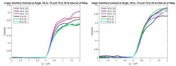
Figure 21 Statistical Averages of Vorticity about Angle

ϕ

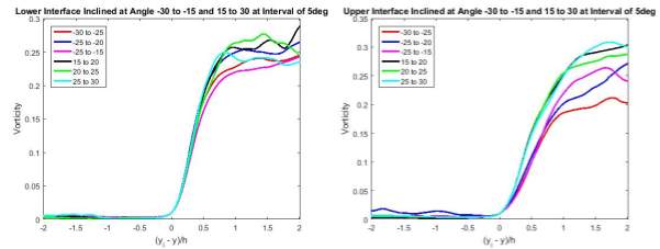
Figure 22 Statistical Averages of Vorticity about Angle

ψ

From the results shown in Figure 21 and 22, the vorticity experienced a sharp jump at the interface as expected, before settling down at approximately between 0.2 and 0.3 moving into the turbulent region. The gradient of the vorticity jump at the upper interface was observed to be slightly gentler as compared to the gradient at the lower interface. This phenomenon can be due to the difference in flow velocity in the irrotational region. Moving at faster velocity could require longer duration and space for the turbulent flow to induce vorticity into the irrotational region along the interface through nibbling.

In contrast to the statistical averages in the 2D cases (Figure 17 and 19), the behaviours of the vorticity across both interfaces in both 2D and 3D scenario appeared to be almost identical. Possible reasoning to such findings could be the magnitude of the vorticity were used, instead of the individual components to compute the statistical averages. Results may signify the reason why most past researches and studies focused only on two-dimensions of the flow instead, as it produces identical results when considering three-dimensions of the flow and saves more time and cost for the research.

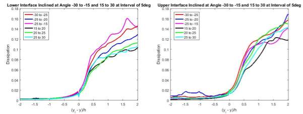
Figure 23 Statistical Averages of Turbulence Kinetic Energy Dissipation about Angle

ϕ

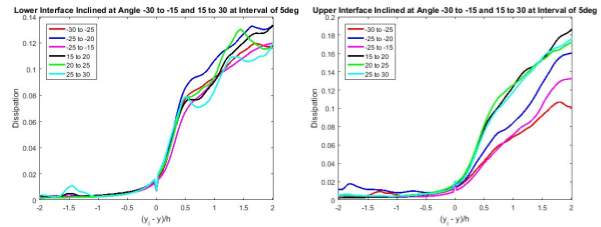
Figure 24 Statistical Averages of Turbulence Kinetic Energy Dissipation about Angle

ψ

Likewise, the turbulence kinetic energy dissipation varied almost identically as observed in the 2D cases (Figure 18 and 20). The turbulence kinetic energy dissipation experienced a sharp decrease (increase) moving across the lower (upper) interface. These increments /decrements were observed at all orientations of the normal (Figure 22 and 23).

Looking at the statistical averages of the velocity in Figure 25 and 26, significant changes in gradient were observed at the interface and at a small distance into the turbulent flow. At the interface, the irrotational flow gained vorticity from the turbulent region, affecting the entrainment velocity of the flow. As mentioned previously, entrainment velocity varies in magnitude and direction. At the lower (upper) interface, the velocity experienced a sharp increase (decrease) moving into the turbulent region. At a small distance into the turbulent region, a second change in gradient could be observed. This distance from the interface at which the second change in gradient was observed indicates the thickness of the interface. With the angles of the normal vector selected for this study not oriented very steeply, it suggested that the normal vector may not cut very deeply into the interface, thus normal vector at different angles may present different interface thickness and different gradient changes, which may not be clearly represented in the results.

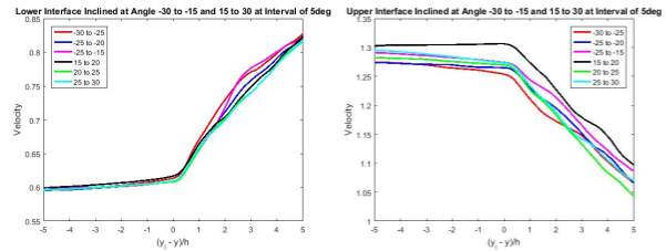
Figure 25 Statistical Averages of Velocity about Angle

ϕ

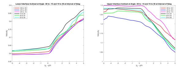
Figure 26 Statistical Averages of Velocity about Angle

ψ

Correlation of Statistical Averages

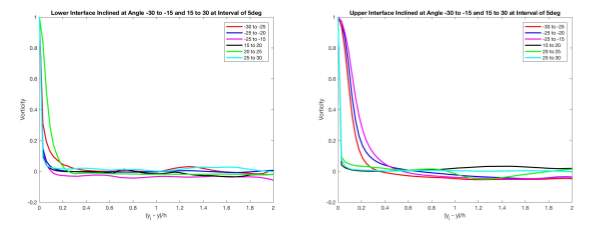
Figure 27 Statistical Correlation Averages of Velocity about Angle

ϕ

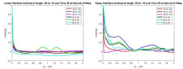
Figure 28 Statistical Correlation Averages of Vorticity about Angle

ψ

The local vorticity magnitude can be expressed in terms of the mean vorticity component and the fluctuating component (i.e.

ω=ω̅+ω’).  The Pearson Correlation Coefficient (PCC) between the vorticity fluctuation at the interface and at a distance away from the interface was computed for both angles,

ϕand

ψ, and depicted in Figure 27 and 28. As expected, steep descents were observed at both interface and the coefficient reaches zero after a short distance from the interface, signifies no linear correlation. However, at the upper interface, the correlation coefficient decreases at a less steeper angle, hitting the axis at approximately

yi-y/h≈0.4when the normal vector is oriented at a negative

ϕ. Similarly, at the upper interface when the normal vector is oriented at angle

ψ, the correlation coefficient decreases at a slower and less smooth manner. These results showed that the vorticity is correlated over a longer distance at the upper interface when it is oriented towards the upstream in the streamwise direction and any orientation in the spanwise direction.

Using trapezoidal rule, the PCC were then integrated to determine the length scale at which the flow is correlated to the interface and tabulated below in terms of the Kolmogorov length scale presented earlier.  These results showed that the vorticity in the turbulent region is insignificantly affected by the orientation of the surface and is quickly independent from the lower interface as compared to the upper interface, where entrainment regions or large-scale vortices are more prominent and likely to exist.

Lower Interface		Upper Interface
Angle,ϕ and ψ	Length Scale	Angle,ϕ and ψ	Length Scale
-30≤ϕ/ψ<-25	25.155η	-30≤ϕ/ψ<-25	93.521η
-25≤ϕ/ψ<-20	18.896η	-25≤ϕ/ψ<-20	69.037η
-20≤ϕ/ψ<-15	16.962η	-20≤ϕ/ψ<-15	142.252η
15≤ϕ/ψ<20	17.070η	15≤ϕ/ψ<20	67.895η
20≤ϕ/ψ<25	63.706η	20≤ϕ/ψ<25	29.949η
25≤ϕ/ψ<30	38.037η	25≤ϕ/ψ<30	31.693η

Table 1 Length Scale at the Respective Angles

Likewise, the local velocity of the flow can be expressed in terms of its mean velocity component and fluctuating component (i.e.

v=v̅+v’). Using the same computational methods, the PCC between the velocity fluctuation at the interface and at a distance away from the interface were computed and the results were illustrated in Figure 29 and 30. At the lower interface, it is prominent that the correlation coefficient experienced a sharp decrease in similar gradient at all orientation of the normal vector from a small distance moving into the turbulent region, followed by a change of gradient at

yi-y/h≈1.0while at the upper interface, the correlation coefficients decreased at rather different gradients for both positively- and negatively-oriented normal vector.

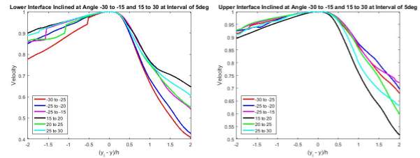
Figure 29 Statistical Correlation Averages of Velocity about Angle

 ϕ

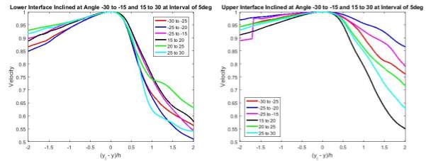
Figure 30 Statistical Correlation Averages of Velocity about Angle

ψ

The gradient at which the correlation coefficient at the lower interface decreased implied a rather low linear relationship between the interface and the turbulent region, showing that the flow was not greatly affected by the presence of any eddies near the lower interface. On the other hand, the different gradients observed at the upper interface suggested that the velocity fluctuations were somewhat correlated to the interface, this may indicate the presence of eddies near the interface when orientated at a certain angle. The correlation coefficient decreases at a much gentler rate when the normal vector is negatively oriented as compared to when the normal vector is positively-oriented. At positive angle, the velocity fluctuations in the turbulent region tend to be less related to the interface when interface is flatter (

ψ→0, ϕ→0). The difference in gradient could also hint the presence of entrainment zone at the upper interface.

Additionally, comparisons were conducted for both between the correlation of the velocity fluctuations with respect to the interface and the correlation with respect to points positioned a distance away from the interface into both irrotational and turbulent regions and between the lower and upper interface at the same regions. Figure 31 illustrated the results of the comparisons among the correlation with respect to irrotational region (red), the interface (black) and turbulent region (blue) at

25≤ϕ<30, and the comparison of similar regions at both the lower and upper interfaces.

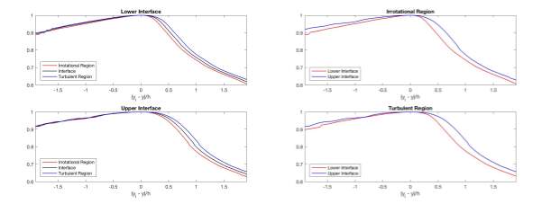
Figure 31 Comparison of Correlation with respect to Different Positions

The results of the comparison presented the correlation coefficients descending at different gradients as compared to the interface. The correlation with respect to the point a small distance into the turbulent region decreased at a gentler rate as compared to the one at the interface. Despite the gradient differences, the correlations at both interfaces appeared to behave into similar fashion. These could be due to the distance of the point taken in consideration for the comparison. The point could lie within the presence of the viscous superlayer as mentioned in the literature, causing the flow to behave similarly as in the turbulent region. With the point in the irrotational region positioned at a small distance away from the interface, the results also suggest that the velocity of the freestream flow is perhaps greatly influenced by the interface once it is in close proximity to the interfaces.

The results shown in Figure 31 also depicted the comparison of the correlations with respect to the irrotational and turbulent regions between the lower and upper interfaces of the turbulent flow. The results suggested that the velocity fluctuations were more correlated to the points in the irrotational and turbulent regions when the freestream flow is moving at a higher velocity. This finding shows that the characteristics of a T/NT interface is not universal, as the upper interface behaves differently from the lower interface.

Positions of Large Vorticity and Dissipation Structures

Within the turbulent region, there are many intermittent small worm-like structures due to high vorticity and high turbulent kinetic energy dissipation rate. Calculations and analyses were done to look at how these worm-like structures are located with respect to the lower and upper interface. Using the vorticity magnitude threshold technique, the contours of the structures are defined. Next, the shortest distance from the centre of mass of each structure to the respective interface were calculated. The mean distances of the structures to the respective interfaces are tabulated and presented in Table 2. It is evident that these structures are approximately twice as distant to the lower interface as to the upper interface. The probability density functions (PDFs) shown in Figure 32 also suggested that most of these high vorticity and dissipation structures are found near the upper interface.

Type of Structures	Lower Interface	Upper Interface
Vorticity	l/h=9.8127	l/h=5.6366
Dissipation	l/h=9.8563	l/h=5.4743

Table 2 Average Distance of the Structures to the Respective Interfaces

Figure 32 Probability Density Functions of the Distances of High Vorticity and Dissipation Structures

The PDF for the distances of the structures to the lower interface resembles much like a Gaussian distribution, where most of the structures found to be located approximately between

l/h≈5and

l/h≈12.5away from the lower interface. On the contrary, the PDF for the distances of the structures to the upper interface is observed to be a positive skewed distribution, showing most of the structures are nearer to the upper interface. Comparatively, the high vorticity structures tend to be nearer to the upper interface than the high dissipation structures; likewise, this is also observed in the PDF for the lower interface.

Conclusion

Detailed studies using the direct numerical studies data of a mixing layer and the low vorticity magnitude threshold technique were conducted to look at the characteristics of the flow across surfaces of a turbulent/non-turbulent (T/NT) interface at different orientations. The vorticity statistical averages on the distance from the interface achieved using the proposed methodology are in good agreement with the results presented from studies in the past, considering the difference in flow parameters and computational model. Results presented in this numerical study exhibited a significant jump in the vorticity and turbulence kinetic energy dissipation across the T/NT interface and a gradient change in the velocity profile of the flow moving from the irrotational region towards the core of the turbulence. It is shown that the positions of the interface evolve in a rather linear manner and the flow expands in thickness in the streamwise direction.

Comparison of results obtained by analysing two-dimensions and three-dimensions of the flow revealed that the results achieved in both scenarios are similar. This can be the reason why most researches and studies focus only on the flow in two-dimensional condition instead, as time and costs of studies can be greatly saved and reduced. Statistical averages on the individual vorticity and velocity components, i.e. tangential vorticity component,

ωz, and streamwise velocity component,

ux, can be further studied to find out the similarities and differences of the characteristic of the flow across the interface in both scenarios.

Correlation of the flow with respect to the interface was also studied. It is evident that the flow is better correlated at the upper interface than at the lower interface. The critical distance at which the flow at the upper interface loses correlation is significantly greater than that at the lower interface regardless of the orientation of the interface. The similar behaviour in the correlation can be due the point lying in the viscous superlayer. Further work can be done by looking at the correlation as the point moves further away from the interface.

Lastly, it is shown that the small worm-like structures in the turbulent flow due to high vorticity and turbulence kinetic energy dissipation tends to be located near the upper interface; the distance of these high magnitude structure to the lower interface follows a Gaussian distribution whereas the distance to the upper interface follows a positively skewed distribution.