Abstract— This paper reviews the ultrasound wave and its application in photoacoustic imaging. Photoacoustic imaging, as a newly developed biomedical imaging technique, can overcome challenges of conventional optical imaging techniques, provide images with high resolution and large penetration depth. In this paper, the background and principle of photoacoustic imaging is introduced. Acoustic wave generation and propagation in photoacoustic imaging is studied and presented. A photoacoustic imaging system and its components, especially the ultrasound detector, is introduced. By taking piezoelectric micromachined ultrasonic transducer (pMUT) as an example, lumped element model (LEM) of the ultrasonic transducer is studied and presented.  The challenges of photoacoustic imaging are also discussed at last.

Index Terms— Photoacoustic, ultrasound, imaging, transducer

I.     INTRODUCTION

ltrasound refers to acoustic waves with frequencies higher than 20 kHz. Applications of ultrasound include gesture recognition [1], range finding (50-300 kHz) [2], medical imaging (5-10 MHz) [3] and fingerprint sensor (10-15 MHz) [4]. Photoacoustic imaging, as one ultrasound application in medical imaging, is a newly developed technology that can create multiscale and multicontrast images of living biological structures ranging from organelles to organs [5]. It integrates the rich optical contrast with high spatial resolution and large imaging depth by detecting photoacoustic pressure generated by thermoelastic expansion following the absorption of optical energy [6]. Photoacoustic imaging has a great significance in biomedical research, including functional imaging, brain lesion detection, hemodynamics monitoring and breast cancer diagnosis.

Conventional pure optical imaging techniques form images based on the spatial variation in the optical properties of samples, such as the reflection, absorption, emission, scattering properties etc. For example, optical coherence tomography (OCT) was developed based on low coherence interferometry. It uses low coherence light (typically near-infrared light) to capture high resolution images from optical scattering media. The typical resolution of an OCT system is as high as 1 to 10 µm. Another imaging technique, confocal microscopy, uses a point source and a conjugate pinhole to block out of focus light in image formation, which can achieve optical images with high resolution and high contrast. Some other optical imaging

techniques, such as fluorescence molecular tomography, two photon imaging technique etc., are also developed and applied in biomedical studies. A typical optical imaging system with components is shown in the Fig. 1.

   

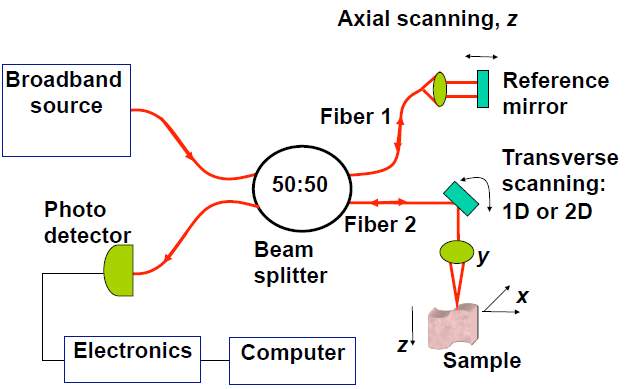
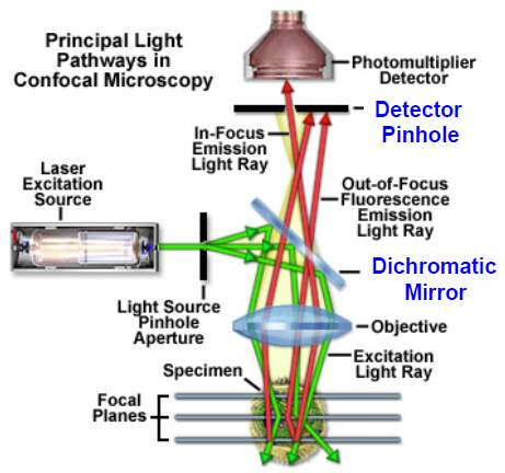
Fig. 1. Diagram of OCT system and fluorescence confocal microscopy system.

There are two main challenges for traditional pure optics imaging techniques, diffraction and diffusion. Diffraction can limit the spatial resolution and diffusion will limit the penetration depth. Besides, when the light propagates in tissues, both absorption and scattering would generate losses. Based on the Beer-Lambert’s Law, the total intensity is attenuated exponentially with the imaging distance and thus the penetration depth is greatly dropped.

However, photoacoustic imaging can overcome these limitations and possess several unique advantages. In photoacoustic imaging, pulse lasers are used to generate the photoacoustic wave. There is still diffusion of the light, but photons diffused inside the tissue are useful photons because all the photons can be absorbed by the targets and the absorbed energy will be converted to acoustic signals. Based on this, even though the light is diffused without any detail, the tissue absorbing it is sharply defined and will provide an equally well-defined ultrasound wave that can be detected. Besides, the scattering of acoustic signal inside a tissue is 100 times weaker than that of light. Because of these, photoacoustic imaging  technique can have a large imaging depth with a high resolution. As shown in Fig. 2, photoacoustic imaging can achieve millimeter imaging depth with a resolution of tens of micrometer.

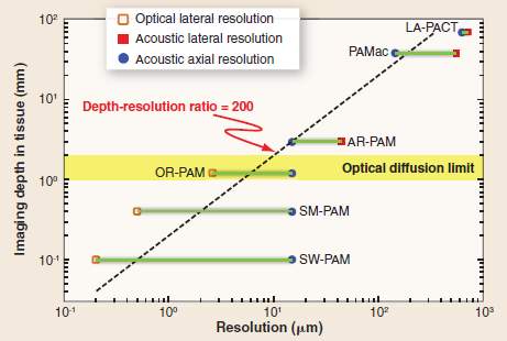
Fig. 2. Imaging depth versus spatial resolution in photoacoustic imaging[5].

There are two main types of photoacoustic imaging modalities, reconstruction based photoacoustic tomography and photoacoustic microscopy. The former one is the traditional mode of photoacoustic imaging. Reconstruction based photoacoustic imaging is the most commonly used and least restrictive photoacoustic imaging technique. A lot of methods, such as back-projection, Fourier transform, P-transform, k-wave method and finite element method have been developed to reconstruct the photoacoustic images from the detected signals. For photoacoustic microscopy, a focused laser beam or a focused transducer with mechanically scanning is used to form the photoacoustic images without any reconstruction algorithms [7]

During last decades, a lot of research on photoacoustic imaging has been presented. L. Xi et al. demonstrated a photoacoustic tomography system within a miniaturized MEMS probe that was practical for intraoperative tumor imaging [8].  C. Kim et al. presented a deeply penetrated in vivo photoacoustic imaging system using a hand-held photoacoustic probe integrated with a clinical ultrasound array [9], as shown in Fig. 3. Transducer arrays with high density of elements were also applied in the photoacoustic imaging system, B. Yin et al. built a fast photoacoustic imaging system based on a 320-elemet linear transducer array, which provided an efficient and convenient method for photoacoustic imaging [10].

Fig. 3. Integrated photoacoustic and ultrasound imaging system with a clinical ultrasound array probe [9].

Real-time photoacoustic imaging systems were also developed, which has potential applications in functional photoacoustic tomographic imaging and small animal studies.  J. Gamelin et al. presented a photoacoustic tomography system using a ring shape ultrasound transducer array with 512 elements, which achieved real-time imaging [11]. As shown in the Fig. 4, the photoacoustic imaging system includes laser source, lens, motor-controlled sample stage and transducer arrays. Data acquired from the acquisition computer are transferred to the FPGA and then processed to form the real time photoacoustic images.

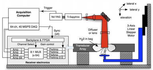
Fig. 4. Diagram of a photoacoustic system [11].

The laser used in their experiment setup provides 8-12 ns pulses at 15 Hz with wavelength tunable from 700 to 950 nm. The transducer array consists of 512 elements and has a center frequency of 5 MHz. Finally, real-time photoacoustic images were formed with a sub-200 µm lateral resolution and a corresponding 0.6-2.5 mm elevation resolution achieved.  The in vivo photoacoustic images of brain vasculature of a mouse are shown in Fig. 5.

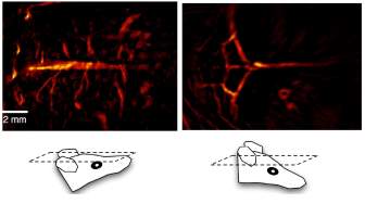
Fig. 5. In vivo photoacoustic images of brain vasculature [11].

II.   Photoacoustic effect

Photoacoustic imaging systems were developed based on the photoacoustic effect. The study of the photoacoustic effect has a long history and it dates back to 1880. When Alexander Graham Bell was experimenting with long distance sound transmission, he observed sound generation due to the absorption of the modulated sunlight and first discovered the photoacoustic effect. After that, photoacoustic effect in gas and liquids were also observed by other researchers. The research on photoacoustic and its applications starts to increase rapidly after the laser was developed in 1960s. Until the mid-1990s, photoacoustic effect starts to be employed in biomedical imaging and develops quickly.

Photoacoustic (PA) effect, also referred as optoacoustic (OA) effect, describes the acoustic wave generation by modulated optical radiation. In a broader sense, photoacoustic can mean the generation of the acoustic waves or other thermoelastic effects by any other types of energetic radiation, including electromagnetic radiation from radio frequency to x ray, electrons, protons, ions and other particles [13]. After optical absorption, the sample is heated due to the “photothermal effect,” which directly caused the temperature rise on the sample. This temperature rise will produce an intimal pressure increase and generates an ultrasound wave. The acoustic wave will then propagate and detected by an ultrasonic transducer or transducer arrays at the surface. Fig. 6 shows a pulsed photoacoustic effect with the absorption of the optical energy and induced ultrasound wave. In order to obtain the photoacoustic effect, the light intensity must vary, either periodically (modulated light) or as a single flash (pulsed light). Normally, nanoseconds laser pulses (around 5 to 15 ns) are used to generate the photoacoustic effect. The temperature increase on the tissue caused by the photoacoustic effect is also very low and won’t cause any damage on the issue.

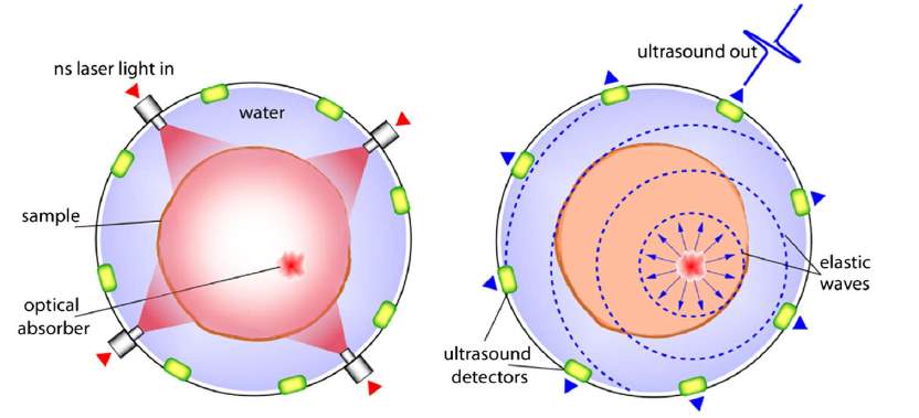
Fig. 6. Schematic of the pulsed photoacoustic effect [10].

III. Photoacoustic wave theory

Photoacoustic generation can be classified to two types according to their excitation modes: the continuous-wave modulation mode and pulsed mode. In the continuous mode, the excitation beam is modulated near a 50% duty cycle while in the pulsed mode, the excitation beam has a very low duty cycle with a very high peak power [13]. Continuous-wave modulation mode has low photoacoustic generation efficiency and low frequency transducers are usually used. Thermal diffusion effects are also important in continuous-wave modulation mode. However, photoacoustic generation efficiency is high in pulsed mode and high frequency transducers are required. Thermal diffusion effects are usually negligible in pulsed mode.

In photoacoustic generation, impulsive heating is assumed and requires that the acoustic propagation time is small compared with the length scale of the heated volume [15]. Then induced acoustic pressure

p0rat a point

ris expressed as:

p0r=γHr

(1)

where

p0is the pressure of the optically induced initial acoustic wave at the point r,

γis known as the Gruneisen coefficient, a dimensionless thermodynamic constant that measures the conversion efficiency of heat energy.

Hris the absorbed optical energy.

The Gruneisen coefficient

γis given by the:

γ=βc2Cp

(2)

where

βis the volume thermal expansivity, c is the sound speed and

Cpis the specific heat capacity at a constant pressure.

The absorbed optical energy distribution H(r) is given by the product of the local absorption coefficient

μarand the optical fluence

∅ r;μa, μs, g:

p0r=γμar∅ r;μa, μs, g

(3)

where

μsis the scattering coefficient and

gis the anisotropy factor.

As the equation shows, photoacoustic pressure

p0rdepends on many parameters related to mechanical, thermodynamic and optical properties. Different types of tissues have different optical absorption and scattering properties, so that a high contrast photoacoustic image can be formed.

More specifically, thermal acoustic wave propagation can be described by the following equation [17]:

(

∇2-1c2∂2∂t2) p(r, t)=-βCp∂It∂tA(r)                      (4)

where

pr, tis the thermoacoustic pressure at position r and time t, c is the sound speed,

βis the isobaric volume expansion coefficient,

Cpis the heat capacity,

Itis the temporal profile of the microwave pulse and

Aris the fractional energy-absorption per unit volume of soft tissue at the position r.

Photoacoustic wave equation has been well studied and wave solution has been presented. G. J. Diebold et al. investigated the photoacoustic effect in fluids and studied the photoacoustic pressure in one, two and three dimensions for short-pulse excitation conditions [18]. By employing Green’s-function solution for the velocity potential, the solution of the photoacoustic wave equation is presented.

Based on the Lambert-Beer law and rectangle function, impulse response of the photoacoustic system was obtained and convoluted with the exciting pulse to acquire the photoacoustic wave pressure. In this method, D. Cywiak et al. studied the general solution of the one-dimensional photoacoustic wave equation [19]. The dependent relationship between the photoacoustic pressure and the laser pulse duration is also studied and presented.

Here, the typical solution of a photoacoustic wave equation in one-dimension will be reviewed and derived step by step as the following:

The photoacoustic wave equation expressed in terms of the velocity potential is expressed as:

∇2φr,t-1c2∂2φr,t∂t2=βρCpHr,t

(5)

where

φr,tis the velocity potential, c is the sound speed,

ρis the density of the absorber in equilibrium,

βis the thermal expansion coefficient,

Cpis the specific heat capacity at a constant pressure.

Hr,tis the energy density per unit time distributed within the heat region during the radiation.

The pressure profile of the photoacoustic wave can be expressed as:

Pr,t=-ρ∂φr,t∂t

(6)

where P(r,t) is the pressure profile of the acoustic wave.

Next, we will calculate the energy density distribution

Hr,ton the absorber. In the absorption model shown in the Fig. 7, we assume that the laser spot size is much larger than the optical absorption length across the absorber, so that the shape of the sound source can be regarded as a plane. Also, we assume that the energy distribution within the thickness of the absorber is dominated by Lambert-Beer’s Law. If the laser beam hit the absorber at

z=z0, then the energy distribution inside the absorber per unit time can be expressed as:

Hx,y,z;t=αQx,y,z0exp⁡-αz0-zft           (7)

where

αis the absorption coefficient of the heated region.

Qx,y,z0is the laser energy hit the absorber at

z0.

ftis the temporal profile of the laser beam.

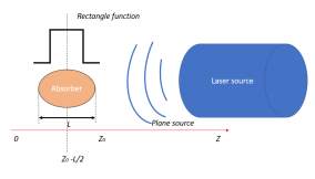
Fig. 7.  Absorption model used in solution.

Consider the thickness L of the absorber, a rectangle function

h zcentered at

z=z0-L2is applied and Eq. 7 is modified as:

Hx,y,z;t=αQx,y,z0exp⁡-αz0-zhz-z0-L2Lft

(8)

To obtain the solution of the photoacoustic wave equation, Green’s function is used. Green’s function describes the impulse response of an inhomogeneous linear differential equation defined in a domain with specified initial conditions or boundary conditions. By using Green’s function solution, the differential equation of Eq. 5 to be solved is:

∂2∂z2Gz,t,z’,t’-1c2∂2Gz,t,z’,t’∂t2=δz-z’δt-t’

(9)

where

Gz,t,z’,t’represents the Green’s function.

The solution of Eq. 5 in terms of Green’s function is:

φz,t=βρCp∫-∞+∞∫0+∞Gz,t,z’,t’Hz’,t’dt’dz’

(10)

In one dimension, the Green’s function can be obtained after integration:

 

Gz,t,z’,t’=-c2ut-t’+z-z’c,z>z’

Gz,t,z’,t’=-c2ut-t’-z-z’c,z<z’

(11)

where u(t) is the Heaviside function.

By substituting Eq. 11 into Eq. 10 and using the Eq. 6, the pressure profile is obtained as:

Pz,t=cβ2Cp∫-∞zHz’,t-z-z’cdz’+cβ2Cp ∫-∞zHz’,t+z-z’cdz’

(12)

In Eq. 12, the first term on the right side represents a right running wave and the second term represents the left running wave.

For an impulse input, the temporal profile of the laser beam is defined as:

ft=δt

(13)

where

δt  is the Dirac delta function.

Finally, applying Eq. 13 into Eq. 12, the impulse response for a plane sample is obtained as:

Pz,t=p02ut{exp-αct-zcht-zc-L2cLc

+expαct+zcht+zc+L2cLc

}                                               (14)

where

P0=c2βαQ0Cpand h is the rectangle function as mentioned above.

z0=0is chosen for simplicity.

With the photoacoustic wave solution and choose typical values for those constants, the photoacoustic wave pressure is studied both by simulation and experiments. As shown in Fig.  8, the profile of the photoacoustic wave pressure will tend to be a Gaussian distribution with the pulse duration increase and the width is given by the laser pulse duration. It’s also seen clearly form the figure that with increase of the time duration, the amplitude of the photoacoustic wave pressure will decrease, which is an expected result of the Lambert-Beer’s absorption law.

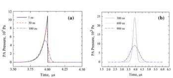
Fig. 8. Photoacoustic wave pressure vs. different        values of the pulse duration [19].

IV.     Photoacoustic imaging

Photoacoustic imaging is a promising biomedical imaging technique. It combines the high contrast of the pure optics imaging modalities with the high ratio of imaging depth to spatial resolution of the ultrasound. Besides, it won’t cause potential safety issues due to the thermal heating or high-pressure waves. During the photoacoustic imaging studies, short pulsed laser is commonly used to generate the ultrasound waves. In the case of the optical excitation, temperature increase caused by the conversion of the absorbed optical energy is very small (approximately less than 0.1 K), much below the temperature increase required to cause the physical damage or physiological changes to tissue. The initial acoustic pressure induced by this thermal expansion also has a low amplitude (less than 10 kPa).

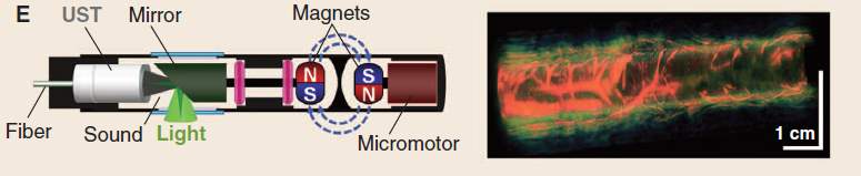
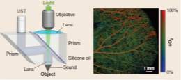
Fig.9. Photoacoustic imaging probe with in vivo images[5].

1. Spatial resolution

The spatial resolution of the photoacoustic imaging technique depends directly on the frequency of the acoustic wave. In photoacoustic imaging, with the use of nanosecond laser pulses, acoustic waves are excited with frequencies ranging from tens to hundreds of megahertz. Acoustic attenuation, bandwidth, element and area of the ultrasonic detectors are also factors that can limit the ultimate spatial resolution. H. Zhang et al. has proposed a high-resolution functional photoacoustic microscopy for in vivo imaging [14]. By using a 6-ns laser pulse from a Nd: YAG laser and a 50 MHz central frequency ultrasonic transducer, this PAM can construct

images with a 15 µm axial resolution and a 45 µm lateral resolution in its focal zone.

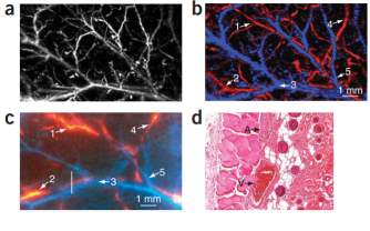
Fig. 10. Functional images by a photoacoustic microscopy in vivo in a rat [14].

2. Penetration depth

The penetration depth of the photoacoustic imaging technique is limited by both optical and acoustical attenuation. However, for most soft tissues, although acoustic attenuation is significant, it is optical attenuation that dominates [15]. Optical attenuation depends on both the absorption and scattering, and it’s strongly wavelength dependent, as shown in the Fig. 11. In homogeneous scattering media, the penetration depth is defined by

1μeff, at which depth the irradiance has decreased by 1/e.

μeffis called the effective attenuation coefficient.

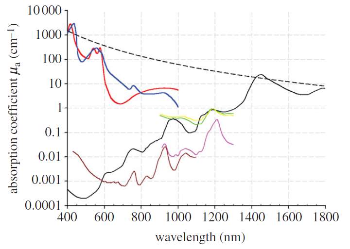
Fig. 11. Wavelength dependent absorption coefficient of different types of tissues [15].

3. Categories of photoacoustic imaging

There are three categories of photoacoustic imaging that are commonly used: photoacoustic tomography (PAT), photoacoustic microscopy and its variants.

Photoacoustic tomography (PAT) is an early developed photoacoustic imaging mode. It is the most general and least restrictive photoacoustic imaging approach. In PAT, a large diameter laser beam is required to illuminate the full field. The light penetrates deeply and strongly scattered. Tissues illuminated absorb the optical energy and generate the ultrasound waves, which propagate and detected by the mechanically scanned ultrasonic transducer or transducer arrays. The time-varying detected ultrasound signals are saved and used to reconstruct the three-dimension images.

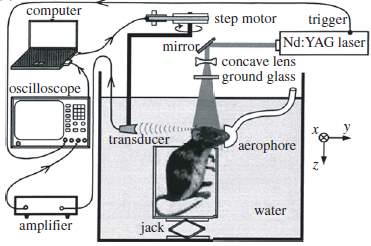
Fig.12.  PAT cylindrical scanner for small animal brain imaging [15].

Photoacoustic microscopy refers to techniques that photoacoustic images are formed by mechanically scanning the focused laser beam or the focused ultrasound transducer. The image is formed directly from the set of acquired A-lines, without any reconstruction as photoacoustic tomography.

For photoacoustic microscopy, they are classified to two types, optical-resolution photoacoustic microscopy (ORPAM) and acoustic-resolution photoacoustic microscopy (ARPAM). If a focused laser beam is used, it is named ORPAM. If using a focused transducer without light beam focusing, it is termed ARPAM. Typically, the resolution for ORPAM is from sub-micro to several micrometers. But due to the penetration limit of the highly focused light beam, the imaging depth of ORPAM is limited to be less than 1mm, which makes it difficult for ORPAM to be applied in cancer research if the tumor lies deep beneath the surface. What’s more, ORPAM is fundamentally sensitive to samples with good optical absorption so that it has a limitation to image tissues with low absorption contrast.

By using a single mechanically rotated focused ultrasonic transducer to map the photoacoustic signals, ARPAM is achieved. For ARPAM, the resolution varies from 30 µm to 1mm, varies with the aperture of transducers, bandwidth and focal length. Meanwhile, the imaging depth is improved, from several mm to cm [16]. Although the lateral resolution of ARPAM is not as high as that of ORPAM, the imaging depth is greatly improved so that it can detect target much deeper than that of ORPAM. It breaks the penetration depth of ORPAM and has wider applications, such as breast cancer detection, lymph node detection and molecular imaging.

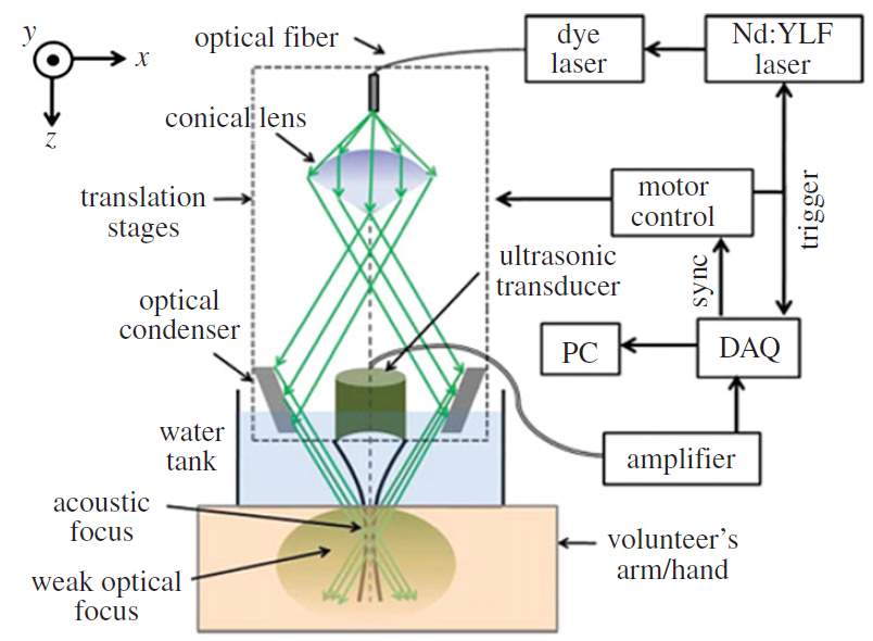
Fig. 13. Schematic of an acoustic-resolution photoacoustic microcopy system[15].

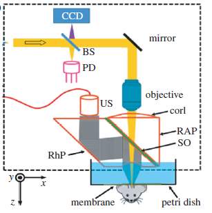
Fig. 14. Schematic of an optical-resolution photoacoustic microscopy scanner[15].

Compared with traditional pulsed-echo ultrasound imaging techniques, photoacoustic imaging has the following different aspects [15]:

1. In photoacoustic imaging, localization can be achieved in reception only for depth greater than approximately 1mm. However, localization can be achieved both in transmitter and receiver by focusing in pulsed-echo ultrasound imaging.
2. The amplitude of photoacoustic pressure (typically less than 10 kPa) is several orders lower than pulsed-echo ultrasound (peak pressure can excess 1 MPa).
3. Photoacoustic imaging represents the initial pressure distribution due to the absorption difference while ultrasound imaging represents the impedance mismatch between different tissues.

V.  Detection of the ultrasound wave

A. Development of the piezoelectric micromachined ultrasonic transducer (pMUT)

In photoacoustic imaging systems, ultrasound transducer is designed as the detector of the ultrasound wave. It works as a transducer to receive the photo-induced ultrasound pressure and convert it to an electrical signal.

Conventional ultrasound transducers consist of lead zirconate titanate (PZT) strips (dimensions on the order of millimeters) that are poled in the thickness direction to operate as thickness mode resonators. In this mode of operation, the frequency of the transducer directly depends on the thickness of the PZT, which can be a limiting factor because geometrical restrictions can conflict with the thickness required for a certain frequency. Furthermore, conventional ultrasound transducers have limitations in their performances, especially in bandwidth due to the acoustic impedance mismatch. Fortunately, many of these problems can potentially be overcome by micromachined ultrasound transducers (MUTs), including capacitive micromachined ultrasound transducers (cMUTs) and piezoelectric micromachined ultrasound transducers (pMUTs). pMUTs, unlike cMUTs that require large bias voltages, also have higher capacitance and lower electrical impedance, so that have been well studied as the ultrasound detector in photoacoustic imaging.

pMUT works on the principle of the piezoelectric effect. It has a structure of sandwich-liked membrane, including piezoelectric layer with top and bottom electrodes, plus one supporting layer. The schematic of a pMUT with the membrane deflection is shown in the Fig. 15. It can work at a flexural vibration mode. When the pMUT receive an acoustic signal and vibrate the membrane, charges will be generated and accumulated on the top and bottom electrodes, which will induce electric potential as the output signal.

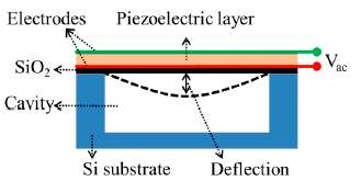
Fig.15. Structure of a pMUT [23].

In recent years, a lot of studies have presented different kinds of micromachined ultrasound transducers based on piezoelectric materials and advanced fabrication process.

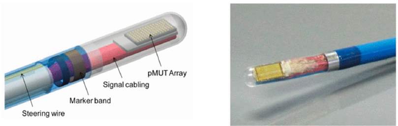
Fig.16. A photoacoustic imaging probe using a pMUT array [23].

Varies of pMUTs or pMUT arrays have been presented with sol-gel PZT, sputtering PZT and AlN [24] to achieve different frequency range and different sensitivities. The typical resonant frequencies of the pMUT can range from a few megahertz to several tens of megahertz. Y. Lu et al. proposed high fill-factor pMUT arrays with two types of piezoelectric materials, PZT and AlN.  A large dynamic displacement of 316 nm/V at 11 MHz in air and a high electromechanical coupling

kt2=12.5%are achieved by PZT pMUTs [24].

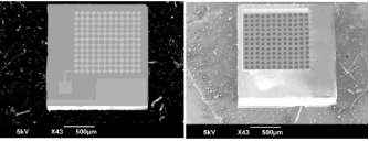
Fig.17.  SEM of a fabricated pMUT array [25]

B. Lumped element model (LEM) of the pMUT

Lumped element model is widely used to analyze the multi-energy domain systems. The lumped element model, also called lumped parameter model or lumped component model, simplifies the description of the behavior of spatially distributed physical systems under the lumped assumption. When the characteristic length scales of the governing physical phenomena are much larger than the geometric dimension of the interest, the partial differential equation (PDEs) of continuous (infinite dimensional) time and space model of the physical system can be simplified into a set of ordinary differentia equations (ODEs) with a finite number of parameters. This approach provides a simple and effective method to analyze the dynamic responses of the system and it has been widely used in electrical systems, mechanical multibody systems, heat transfer and acoustic systems, etc.

The lumped element modeling technique provides efficient predictions of the behavior of Multiphysics system. For acoustic devices such as microphone, speaker and pMUT, the lumped element model (LEM) has been well studied and presented [21] [26][27]. Three equivalent circuit models of the transducers are shown in the Fig. 13 and they can be converted between each other. In the circuit representation,

Zeis the electrical feedthrough,

Zmis the mechanical impedance,

Zais the acoustic load, and

ƞis the electromechanical transduction ratio.

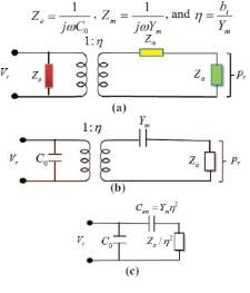
Fig. 18. Three equivalent circuit models of the transducer [27].

In the LEM analysis, membrane, cavity and vent hole of an ultrasonic transducer can be represented by the equivalent mass, spring and damper system, or capacitance, resistance and inductance in an electrical circuit. An equivalent circuit for a pMUT can be built with lumped elements, as shown in the Fig. 14 and Fig. 15.

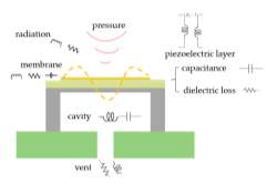
Fig. 19. pMUT structure with lumped parameters.

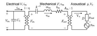
Fig. 20. Electrical, mechanial and acoustical model of the ultrasound transducer [28].

By combining the mechanical and acoustical models, a simplified circuit is shown in the Fig. 21. It includes acoustic domain and electrical domain, coupled by the piezoelectric layer, which is represented by a tranformer with the transfer ratio

∅ain the circuit. In the acoustic domain, acousti pressure

p  [Pa] is analogous to the voltage and the volume velocity

q[m³/s] is used to analog current. Acoustic impedance is defined as

pq. The particle velocity is

u[m/s] and the cross area is S [

m2].

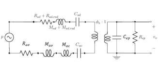
Fig. 21. The equivalent circuit of the pMUT LEM.

The acoustic impedance of the mass is expressed as:

pq=fmassSSu=Mu̇S2u=jωMS2=jωMac

(15)

Mac=MS2

(16)

where M is the mass and

Macis called the acoustic inertance.

Similarly, acoustic stiffness

Kac=KS2acoustic compliance

Cac=1Kacis also defined:

pq=fspringSSu=KxS2ẋ=KjωS2=Kacjω=1jωCac

(17)

Comparing with the formula

ei=jωL,    ei=1jωCin electrical circuit theory, inductance

Land

Mac, C and

Cacare analogies in lumped element model (LEM). Finally, the acoustic resistance

Rac, which may be due to one of several dumping mechanisms, is analogous to electrical resistance R.

Based on the acoustic theory, for a short closed tube or cavity of length l and cross-sectional area S, the volume V=ls. The acoustic impedance is given by:

Zac=ρ0c02jωV+jωρ0V3S2=1jωCac+jωMac

(18)

Cac=Vρ0c02

(19)

Mac=ρ0V3S2

(20)

For the diaphragm, the compliance and inertance are given by:

Cad=∫0R2πrwrdrP|V=0

(21)

Mad=MeqS2=∫0R2πrρAwr2dr∆V2|V=0

(22)

where w(r) is the distributed deflection of the diaphragm and

∆V=∫0R2πrwrdr.

For the coupling between the diaphragm and air on the free side, the radiation mass

Mad,radand resistance

Rad,radare defined to model them.

Rad,rad=kR2ρ0c2A

(23)

Mad,rad=8kRρ0c3πωA

(24)

The vent hole is represented as a resistor and an inertance, which are given by the following equations:

Rav=8lμπa4

(25)

Mav=ρ0 lπa2

(26)

where

lis the length of the vent,

μis viscosity of air and

ais radius of the vent.

In electrical domain, the capacitance and resistance (representing dielectric loss) of the piezoelectric layer are defined as:

Cep=ϵπr2hp

(27)

Rep=ρphpA

(28)

where

ϵis the dielectric permittivity,

ρpis the resistivity of the piezoelectric material,

hpis the thickness of the piezoelectric layer and A is the area of the piezoelectric layer.

Finally, the coupling between the acoustical domain and electrical domain is represented by a transformer with a transfer ratio

∅a[Pa/V] and given by:

∅a=daCad

(29)

where

da=∆V̅|p=0V  [

m3V],

Cad=∆V̅|V=0P[

m3Pa].

∆V̅is the volume displacement, V is the applied voltage and P is the applied pressure.

After lumped elements were defined and calculated based on design parameters, the transfer function of the equivalent circuit can be derived from the equivalent circuit (Fig. 16) and expressed as:

Hf=v0p=iZep∅aiZep+i∅aZad+Zac+Rav=∅aZep∅a2Zep+Zad+Zac+Rav

(30)

where

Zad,

Zac,

Rav,

Zepare impedances of the diaphragm, cavity, vent hole and piezoelectric layer,

∅ais the transfer ratio and

iis the flow in the circuit.

The transfer function of the circuit represents the sensitivity (V/Pa) of the pMUT. By programming in Matlab, the frequency response of the pMUT can be plotted, as shown in the Fig. 22.

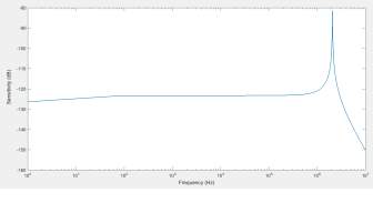
Fig. 22. Predicted frequency response of the pMUT based on LEM.

Based on the plot, the performance of the designed pMUT can be predicted. The resonant frequency, bandwidth, quality factor and the sensitivity can be analyzed. Effects of the cavity, vent and parasitic capacitance on the performance can also be understood and optimized based on the LEM.

VI. Challenges of the photoacoustic imaging

Although photoacoustic imaging has much advantages over those conventional imaging techniques. The feasibility of obtaining high contrast, high resolution three-dimensional images with large depth through photoacoustic imaging has been demonstrated. But its practical use is still limited by many factors. The presentations of the photoacoustic imaging in the last decades are also focused on experimental studies. There are still some challenges that inhibit the widely application of the photoacoustic imaging.

One challenge in terms of instrument is the lack of highly sensitive broadband ultrasound receivers for photoacoustic detection. A common problem is that the characteristic impedance of the piezoelectric element is very different from that of the air. Such a large impedance mismatch exists between them and cause the large reflection. A quarter-wavelength thick matching layer at the frequency of interest is thus usually used to solve this. However, the application of the impedance matching layer would limit the overall bandwidth of the transducer [28]. But the matching layer is still required in most of devices currently. This may be solved by advanced piezoelectric material and new design approaches in the future.

The lack of suitable laser systems is also a limitation for the clinical application of the photoacoustic imaging. Currently, commercially Q-switched lasers, Ti Sapphire and dye lasers are used in the photoacoustic imaging research and proved to be effective. However, their large size, lack of practical utility and requirement of cooling system inhibit their practical use in photoacoustic imaging applications [15].

VII. Summary

In summary, a review of the photoacoustic imaging from background, principle, categories, imaging systems to challenges has been presented. The advantages of photoacoustic imaging over conventional pure optical imaging techniques are discussed. Differences between photoacoustic imaging and traditional pulsed-echo ultrasound imaging are also compared. Ultrasound waves in the photoacoustic imaging has been studied, including its generation by thermal acoustic effect and detection by the piezoelectric ultrasonic transducers. Lumped element model (LEM) of the piezoelectric ultrasound transducer is also introduced and analyzed. Finally, current challenges that limit the practical application of photoacoustic imaging are reviewed and discussed.

References

1. K. Kalgaonkar and B. Raj, “One-handed gesture recognition using ultrasonic Doppler sonar,” 2009 IEEE International Conference on Acoustics, Speech and Signal Processing, 2009, p.1889-1892.
2. M. Saad, C. Bleakley, S. Dobson, “Robust high-accuracy ultrasonic range measurement system,” IEEE transactions on instrumentation and measurement, 2011, vol.60, no.10, p.3334-3341.
3. A. Sarvazyan et al., “Ahear wave elasticity imaging: a new ultrasonic technology of medical diagnostics,” Ultrasound in Med. & Biol., 1998, vol. 24, no. 9, pp. 1419-1435.
4. Y. Lu et al., “Ultrasonic fingerprint sensor using a piezoelectric micromachined ultrasonic transducer array integrated with complementary metal oxide semiconductor electronics,” Applied Physics Letter, 2015, vol. 106, 263503.
5. L. Wang and S. Hu, “Photoacoustic Tomography: in Vivo Imaging from Organelles to Organs,” Science, vol. 335, no. 6075, pp. 1458–1462, 2012.
6. D. Wang, Y. Wu and J. Xia, “Review on photoacoustic imaging of the

brain using nanoprobes,” Neurophotonics, vol. 3, no. 1, pp. 1-8, 2016.

7. M. Xu and L. V. Wang, “Photoacoustic imaging in biomedicine,” Review of Scientific Instruments, vol. 77, no. 4, 2006.
8. L. Xi et al., “Evaluation of breast tumor margins in vivo with intraoperative photoacoustic imaging,” Optics Express, vol. 20, no. 8, pp. 8726-8731, 2012.
9. C. Kim et al., “Deeply penetrating in vivo photoacoustic imaging using a clinical ultrasound array system,” Biomedical Optics Express, vol. 1, no.1, pp. 279-284, 2010.
10. B. Yin et al., “Fast photoacoustic imaging system based on 320-element linear transducer array,” Physics in Medicine and Biology, vol. 49, pp. 1339-1346, 2004.
11. J. Gamelin et al., “A real-time photoacoustic tomography system for small animals,” Optical Society of America, vol. 17, no. 13, pp. 10489-10589, 2009.
12. S. Manohar and D. Razansky, “Photoacoustics: a historical review,” Advances in Optics and Photonics, vol. 8, no. 4, pp. 587-617, 2016.
13. A. C. Tam, “Applications of photoacoustic sensing techniques,” Review of Modern Physics, vol. 58, no. 2, pp. 381-431, 1986.
14. H. F. Zhang et al., “Functional photoacoustic microscopy for high-resolution and noninvasive in vivo imaging,” Nature Biotechnology, vo. 24, no. 7, pp. 848-851, 2006.
15. P. Beard, “Biomedical photoacoustic imaging,” Interface Focus, vol.1, pp. 602-631, 2011.
16. Lei Xi, “Multi-scale photoacoustic tomography and its applications to cancer research,” thesis, 2012.
17. M. Xu, G. Ku and L. Wang, “Microwave-induced thermoacoustic tomography using multi-sector scanning,” Medical Physics, vol. 28, no. 9, pp. 1958-1963, 2001.
18. G. J. Diebold, T. Sun and M. I. Khan, “Photoacoustic monopole radiation in one, two, and three dimensions,” Physical Review Letters, vol. 67, no. 24, pp. 3384-3387, 1991.
19. D. Cywiak et al., “A one-dimensional solution of the photoacoustic wave equation and its relationship with optical absorption,” Int. J. Thermophys., vol. 34, pp. 1473-1480, 2013.
20. Y. Qiu et al., “Piezoelectric micromachined ultrasound transducer (PMUT) arrays for integrated sensing, actuation and imaging,” Sensors (Switzerland), vol. 15, no. 4, pp. 8020–8041, 2015.
21. M. D. Williams, B. A. Griffin, T. N. Reagan, J. R. Underbrink, and M. Sheplak, “An AlN MEMS piezoelectric microphone for aeroacoustic applications,” Journal of Microelectromechanical Systems, vol. 21, no.2, pp. 270-283, 2012.
22. R. A. Kruger, P. Liu, Y. Fang, and R. Appledorn, “Photoacoustic ultrasound (PAUS)–reconstruction tomography,” Medical Physics, vol. 22, no. 10, pp. 1605-1609, 1995.
23. Y. Qiu et al., “Piezoelectric micromachined ultrasound transducer (PMUT) arrays for integrated sensing, actuation and imaging,” Sensors, vol. 15, pp. 8020-8041, 2015.
24. Y. Lu and D. Horsley, “Modeling, fabrication, and characterization of piezoelectric micromachined ultrasonic transducer arrays bsed on cavity SOI wafers,” Journal of Microelectromechanical Systems, vol. 24, no. 4, pp. 1142-1149, 2015.
25. W. Liao et al., “Piezoelectric micromachined ultrasound transducer array for photoacoustic imaging,” Transducers, 2013.
26. S. Akhbari, F. Sammoura and L. Lin, “An equivalent circuit model for curved piezoelectric micromachined ultrasonic transducers with spherical-shape diaphragms,” IEEE International Ultrasonics Symposium Proceedings, 2014, pp. 301-304.
27. R. Przybyla et al., “In-air ragefinding with an AlN piezoelectric micromachined ultrasound transducer,” IEEE Sensors Journal, vol. 11, no. 11, pp. 2690-2697, 2011.
28. T. H. Gan, D. A. Hutchins, D. R. Billson, and D. W. Schindel, “The use of broadband acoustic transducers and pulse-compression techniques for air-coupled ultrasonic imaging,” Ultrasonics, vol. 39, no. 3, pp. 181–194, 2001.

Haoran Wang is with the Department of Electrical and Computer Engineering, University of Florida, Gainesville, Florida, 32611, USA. (e-mail: wanghaoran@ufl.edu)