CFD Modelling of Venturi Meters At Low Reynolds Numbers

Abstract

This study focused around low Reynolds number flows, between 200 and 20,000, these flows are usually associated with slow moving highly viscous fluids such as oil. CFD was to be used and to be verified by test data. Once the CFD was verified by the test data improvements were then to be made to the design of the venturi so that the discharge coefficient (Cd) could be improved, thus improving the flow measurements within this range. It could be assumed that if the CFD results were consistent with the test data for a regular venturi geometry that the CFD results for the edited geometries would be an accurate representation of the flow effects.

The standard venturi meters were created in ANSYS design modeller in such a way that they could be used axisymmetrically in fluent and were based on engineering drawings that were provided for these purposes. While meshing the domain, a mapped mesh was generated so that the elements within the mesh would be quadrilateral and then sizing was added so that there was a bias towards the wall of the domain.

The CFD was proven to be accurate and the geometry of the venturis were edited. Improvements to the Cd of venturi meters has been achieved, however, these are only marginal improvements and further work is required.

Contents

Introduction

Literature Review

Theoretical Background

CFD Theory

Venturi Theory

Validation of CFD Models

Methodology

Results and Discussion

Modifying The Geometry

Results and Discussion

Conclusions

References

Notations

Notation	Definition
2D	Two Dimensional
A	Area
Cd	Discharge Coefficient
CFD	Computational Fluid Dynamics
D	Pipe Diameter
d	Throat Diameter
P	Pressure
Q	Volume Flow
β	Beta
Δ	Change in…
ρ	Density

Introduction

With the oil industry in decline in recent years and the price per barrel of oil dropping to as low as $48.45 (Ref 1) it has become crucial for the oil industry to save money where ever possible. In recent history, the oil industry has been riding a wave of high oil prices and has not been overly concerned with cost savings, thus they are far behind other industries in this aspect. This study has been carried out as it has been identified that the oil industry could benefit from an improvement in flow measurement devices. This study also focuses around very low Reynolds numbers, between roughly 200-20,000 as this has been identified as a key area in which there is not a vast amount of knowledge or understanding of the accuracy and use of differential pressure flow meters and much of the oil that flows through pipe lines is highly viscous, meaning that the Reynolds numbers will typically fall within this range. Differential pressure flow meters would be an ideal tool for the oil industry as they are relatively cheap, they can be easily calibrated and they are easy to maintain as there are have no moving parts, thus saving money in the long-run. The specific type of flow meter that was looked at during this study was a venturi meter, these would be ideal for such an application as currently the discharge coefficient for a venturi meter is typically between 0.95 and 0.99. Figure 1 illustrates how a venturi meter works, a venturi meter reduces the cross sectional area that the flow can pass through, as a result the velocity of the flow increases and the pressure decreases as described by Bernoulli’s equations. This pressure change is also shown in Figure 1as well as the resulting pressure loss, called “Head loss” in the figure. This pressure loss after the flow meter is reduced by the diverging section of a venturi meter and is one aspect of a venturi that may make a venturi meter more desirable than other types of differential pressure flow meter such as an orifice where there is a larger loss in pressure downstream due to the lack of a divergent section that eases the flow back towards it’s original state.

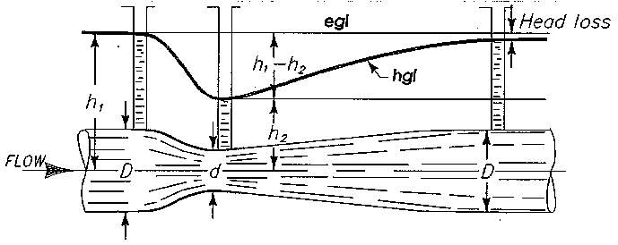
Figure 1: Diagram of Venturi Meter (Ref 2)

Despite the accurate results that can be obtained from venturi meters little is known about how they perform at low Reynolds numbers, the ISO standards that currently exist only accommodate for Reynolds numbers as low as 250,000. (Ref 3) The aims of this study have been to verify the feasibility of CFD modelling of flows at such low Reynolds numbers and to attempt to improve the design of venturi meters for these specific cases using the verified CFD models as the tool to analyse any changes made to the venturi meters. Any improvement that could be made to the accuracy of these flow meters would be of a great advantage to the oil industry as a simple 1% improvement in flow measurement could save the UK’s oil industry £350 million a year (Ref 4).

In this study CFD has been used to plot the behaviour of the discharge coefficient (Cd) as the Reynolds number increases. This has been done to gain a better understanding of how the flow of fluids will behave throughout the laminar, transition and turbulent regions of the flow. The CFD results have been verified through-out by comparing them to test data and using the exact flow characteristics for each different flow within the CFD to ensure a direct comparison could be made. The test data and engineering drawings for the venturis used has been supplied by TUV NEL, a national measurements laboratory, along with the results of the Cd and the Reynolds numbers at each measurement an extensive list of fluid properties has been supplied to ensure accuracy in the modelling of the flow. Two separate fluids were used in this study to measure the effects of Reynolds numbers on the Cd, these were Siptech and Aztec, due to the accuracy of the test data provided the key fluid properties for each fluid did not remain constant as the measurements were adjusted considering any elemental changes present at the time of measurement, such as room temperature, flow temperature and atmospheric changes in pressure. Three separate venturi meters have been examined through all the flow regions to characterise the flow, the venturis range from 0.4β to 0.75β with differing geometries. The results have been given as graphs plotting Cd Vs Reynolds number and show that at these low Reynolds numbers it is crucial to understand how the operating Reynolds number range will affect the performance of the venturi, the numerical procedures used to obtain these results will also be described.

Literature Review

The research carried out has been focused on very small Reynolds numbers and has not only focused on venturi meters but also other forms of differential pressure meters to gain a greater understanding for the behaviour of the fluid flow at these Reynolds number ranges. A large amount of research has been conducted throughout the duration of this study, however, a relatively small amount of information has been available directly concerning fluid flow within the desired range of Reynolds numbers

C.L. Hollingshead (2011) carried out a study into the effects of low to high Reynolds numbers on the flow of oil and water through several different flow meters, including venturi meters. The venturi meters used were multi-stage converging venturis, meaning that instead of a single straight line converging section the venturi meters had two straight converging sections at different angles leading from the pipe to the throat. The study found that at high Reynolds numbers the Cd remained relatively constant with only small fluctuations, however, at low Reynolds numbers the Cd of the flow varied with Reynolds number and as such this range of Reynolds numbers would require flow measurement refinements. The study suggested that more test data should be obtained and a larger range of β values should be examined. (Ref 5)

A study was carried out on the applicability of conventional orifice plates and venturi meters to monitor the rate of oil/water emulsions by R. Pal (1993). The study determined the different Cd values produced by a single orifice plate and a single venturi meter with emulsions of varying concentration of oil, between 0-84.32% The study concluded that Venturi and Orifice meters were viable flow meters for oil and emulsions and that any calibration curve found for any single phased Newtonian fluid is applicable to surfactant stabilized emulsions. (Ref 6)

A study was carried out by B.Pinguet, G.Miller, P.Mosknes and B.Theuveny on the influence of liquid viscosity on multiphase flow meters. The study was conducted to gain an understanding of the performance of differential flow meters when used to measure highly viscous fluids. The issue presented was based on the increasing extraction of heavy oil by the oil industry, these heavy oils are much more viscous than the crude oil that is the standard within the industry. These highly viscous oils have much lower Reynolds numbers, they can also trap regions of less viscous fluid, as these regions pass through a flow meter it can lead to a large miscalculation in the volume flow rate. The study concluded that the highly viscous flows can easily be quantified if the physics of the multiphase flow is considered. It was also demonstrated that in a well-controlled environment that the heavy oil emulsions could be accurately measured with differential pressure meters, even at very low Reynolds numbers. (Ref 7)

M. Ishibashi carried out a study on critical toroidal-throat venturi nozzles covering the boundary-layer transition regime. The study found that there was a correlating equation relating the Cd and Reynolds numbers covering the range of Reynolds numbers within ISO 9300 and that a single equation can replace the two equations detailed within ISO 9300 : 2005. (Ref 8)

NEL also carried out a study into the effects on the Cd in standard and non-standard convergent angles in venturi meters. The study was carried out on large Reynolds numbers when compared to those contained within this project, however, the study found that there were promising results on the uncertainty of the flow measurement when the convergent angle was changed from the standard 21° to 10.5°, other measurements were taken with the convergent angle set to 31.5°, however, these results were deemed to be more unstable. (Ref 9)

Theoretical Background

CFD Theory

Before using any computational tools for any engineering calculations it is important to have an understanding of how the computational models work.

The key equations underlying LES CFD analysis are the Navier stokes equations. The Navier-Stokes equations are only valid when the flows are incompressible, the energy equation adjusts calculations for compressible flow, however, the flow within this study is incompressible, therefore, the Navier-Stokes equations are valid and the energy equations are not required for the calculations. The Navier-Stokes equations are solved simultaneously and are made up of a number of equations including the momentum and continuity equations.  By filtering the continuity and momentum equations we get the following Equation 1and Equation 2 shown below.

∂ρ∂t+∂∂xiρu̅i=0

1

∂∂tρu̅i+∂∂xjρu̅iu̅j=∂∂xjσij-∂p̅∂xi-∂τij∂xj

2

Where

σijis the stress tensor due to molecular viscosity and

τijis defined as the subgrid scale stress. These terms are defined below in Equation 3 and Equation 4.

σij≡μ∂u̅i∂xj+∂u̅j∂xi-23μ∂u̅l∂xlδij

3

τij≡ρuiuj¯-ρu̅iu̅j

4

Newton’s second law states that the forces acting on an object can be calculated through the rate of change of the momentum. This is how the above described momentum equations are used within Fluent, the forces acting on the fluid are firstly calculated using this method, after the forces have been calculated the resulting vectors can be generated. These vectors are then used within the continuity equation.

When a higher level of accuracy is required the second order upwind schemes are used. Quantities at the cell faces are calculated using a multidimensional linear reconstruction approach. By doing this a higher level of accuracy is achieved through a Taylor series expansion of the cell centered solution about the cell centroid. The second order upwind scheme, which was used for the calculation of a number of parameters within the CFD analysis, is described below in Equation 5.

ϕf,  SOU=ϕ+∇ϕr̅

5

Where

ϕfis the face valueof the cells,

ϕis the cell centered value,

∇ϕis the gradient in the upstream cell and

r̅is the displacement vector from the upstream cell centroid to the face centroid. The gradient

∇ϕis also limited so that no new minimums or maximums are introduced during the analysis. (Ref 10)

Within the transition region of the flow the transition k-kl-omega model was used. The k-kl-omega transition model is a three eddy viscosity equation that includes transport equations. These transport equations allow for the calculation of turbulent kinetic energy (

kT), laminar kinetic energy (

kL) and the inverse turbulent time scale (ω). These equations are shown below in Equation 6, Equation 7 and Equation 8 respectively.

DkTDt=PkT+R+RNAT-DT+∂∂xjv+αTαk∂kT∂xj

6

DkLDt=PkL-R-RNAT-DL+∂∂xjv∂kL∂xj

7

DωDt=Cω1ωkTPkT+CωRfW-1ωkTR+RNAT-Cω2ω2+Cω3fωαTfW2kTd3+∂∂xjv+αTαω∂ω∂xj

8

The involvement of laminar and turbulent variations on the mean flow and energy equations via the eddy viscosity and total thermal diffusivity is given in Equation 9and Equation 10.

-uiuj¯=vTOT∂Ui∂xj+∂Uj∂xi-23kTOTδij

9

-uiθ¯=αθ,TOT∂θ∂xi

10

The effective length is given in Equation 11

λeff=MIN(Cλd,λT)

11

Where

λTis given in Equation 12.

λT=kω

12

The small scale energy is defined in Equations 13, 14 and 15.

kT,s=fssfWkT

13

fW=λeffλT

14

fss=e-CssvΩkT2

15

Equation 16 shows how the large scale energy is calculated.

kT,l=kT-kT,s

16

The turbulence production terms generated by turbulent variations are shown in Equation 17.

PkT=vT,sS2

17

The small scale turbulent viscosity is shown in Equation 18.

vT,s=fvfINTCμkT,sλeff

18

Where ,

Cμ=1A0+AsSω

19

fv=1-e-ReT,sAv

20

A damping function required due to the production of turbulence from intermittency is shown in Equations 21 and 22.

fINT=MINkLCINTkTOT,1

21

ReT,s=fW2kTvω

22

In Equation 7

PkLis the production of laminar kinetic energy by large scale turbulent fluctuations, this parameter is defined below in Equation 23.

PkL=vT,lS2

23

vT,1

is the large scale turbulence viscosity and is shown in Equation 24.

vT,1=MINvT,1*,0.5kL+kT,1S

24

When

vT,1*is defined as shown in Equation 25.

vT,1*=fτ,1C11Ωλeff2vkT,1λeff+βTSC12ϕNATd2Ω

25

Equation 24contains a limit that ensures that the realizability of the 2D developing boundary layer is not violated, the time-scale-based damping function

fτ,1is shown below.

fτ,1=1-e-Cτ,1kT,1λeff2Ω2

26

And

βTSfrom Equation 25 is defined as:

βTS=1-e-MAXϕNAT-CTS,crit,02ATS

27

Where,

ϕNAT=d2Ωv

28

The near wall dissipation is calculated using Equations 29and30.

DT=2v∂kT∂xj∂kT∂xj

29

DL=2v∂kL∂xj∂kL∂xj

30

In Equations 6, 7and8 R is the averaged effect of the breakdown of streamwise variations into turbulence during bypass transition, R can be defined as:

R=CRβBPkLωfW

31

Where

βBPis the threshold function that controls the transition process.

βBP=1-e-ϕBPABP

32

ϕBP=MAXKTvΩ-CBP,crit,0

33

Turbulence breaking down caused by inherent instabilities is thought of as a natural transition production tern. This term is defined as:

RNAT=CR,NATβNATkLΩ

34

When,

βNAT=1-e-MAXϕNAT-CNAT,critfNAT,crit,0ANAT

35

and

fNAT,crit=1-eCNCkLdv

36

The intermittency effect from the outer region of the boundary layer can be reduced through the use of ω. The damping equation shown below can be defined from Equation 8.

fω=1-e-0.41λeffλT4

37

The total eddy viscosity and eddy diffusivity from Equations 9and10can be shown as Equations 38and39respectively.

vTOT=vT,svT,l

38

αθ,TOT=fWkTkTOT vT,sPrθ+1-fWCα,θkTλeff

39

The turbulent scalar diffusivity from Equations 6, 7and8 can be written as Equations 40and41.

αT=fvCμ,stdkT,sλeff

40

kTOT=kT+kL

41

A compressibility factor is available within the k-kl-omega transition model, as default it is left switched off, as the flows are incompressible this study this has been left as the default.

The constants for the equations involved in the k-kl-omega model are given below.

A0=4.04, As=2.12, Av=6.75, ABP=0.6

ANAT=200, ATS=200,CBP,crit=1.2, CNC=0.1

CNAT,crit=1250, CINT=0.75, CTS,crit=1000, CR,NAT=0.02

C11=3.4×10-6, C12=1×10-10, CR=0.12, Cα,θ=0.035

CSS=1.5, Cτ,1=4360, Cω1=0.44, Cω2=0.92

Cω3=0.3, CωR=1.5, Cλ=2.495, Cμ,std=0.09

Prθ=0.85, σk=1, σω=1.17

(Ref 10)

The chosen model used to analyse the turbulent flows within this study was the standard k-omega model. The standard k-omega model in Fluent has been based on the Wilcox k-omega model. The Wilcox k-omega model uses modifications for compressibility, shear flow spreading and low Reynolds number effects, which is very applicable for this study. The Wilcox model is, however, relatively weak with respect to the sensitivity of the solutions produced to values of k and omega outside of the shear layer, the model implemented in Fluent has reduced this weakness but it still may have an effect on the results produced, particularly for free shear flows. The k-omega model has been modified many times in recent years, the production terms have been added to the k and omega equations, as a result the overall accuracy of the model for predicting the free shear flows has been improved.

The standard k-omega model is an empirical model based on model transport equations for the turbulence kinetic energy and the specific dissipation rate, which can also be thought of as the ratio of epsilon to k.

The general transport equations for the kinetic energy, k, and the dissipation rate, omega, are shown below in Equations 42and43.

∂∂tρk+∂∂xiρkui=∂∂xjΓk∂k∂xj+Gk-Yk+Sk

42

∂∂tρω+∂∂xiρωui=∂∂xjΓω∂ω∂xj+Gω-Yω+Sω

43

Where

Gkis the generation of turbulent kinetic energy caused by mean velocity gradients,

Gωis the generation of ω.

Γkand

Γωare the diffusivity of k and ω respectively.

Ykand

Yωare the dissipation of k and ω due to turbulence.

Skand

Sωare both user defined terms.

The diffusivities for the k-omega model are shown in Equations 44and45.

Γk=μ+μtσk

44

Γω=μ+μtσω

45

When

σkand

σωare the turbulent Prandtl numbers for k and omega respectively. The turbulent viscosity,

μt, can be computed by combining both k and omega, this is shown in Equation 46.

μt=α*ρkω

46

The low Reynolds number correction factor is generated by

α*. This factor damps the turbulent viscosity causing low Reynolds number correction, this is shown in Equation 47.

α*=α∞*α0*+RetRk1+RetRk

47

Where

Ret=ρkμω

48

Rk=6

49

α0*=βi3

50

βi=0.072

51

It should be noted that for high Reynolds numbers in the k-omega model

α*=α∞*=1.

The production of turbulent kinetic energy can be taken from the transport equation for k, this is shown below in Equation 52.

 

Gk=-ρui’uj’¯∂uj∂xi

52

The production of turbulent kinetic energy can also be calculated in a manner consistent with the Boussinesq hypothesis as shown below.

Gk=μtS2

53

S is the modulus of the mean rate of strain tensor.

Gω

represents the production of ω,

Gωis defined below in Equation 54

Gω=αωkGk

54

When

α=α∞α*α0+RetRω1+RetRω

55

When

Rω=2.95α*and

Retare calculated as shown above in Equations 47and 48.

 

It should be noted that for high Reynolds numbers in the k-omega model

α=α∞=1

.

The turbulence dissipation of k is defined in Equation 56.

 

Yk=ρβ*fβ*kω

56

Where

fβ*=1 1+680Xk21+400Xk2      Xk≤0-Xk>0

57

and

Xk≡1ω3∂k∂xj∂ω∂xj

58

β*=βi*1+ζ*FMt

59

βi*=β∞*415+RetRβ41+RetRβ4

60

ζ*=1.5

61

Rβ=8

62

β∞*=0.09

63

The turbulence dissipation of ω is defined in Equation 64.

Yω=ρβfβω2

64

Where the parameters are defined below.

fβ=1+70Xω1+80Xω

65

Xω=ΩijΩjkSkiβ∞*ω3

66

Ωij=12∂ui∂xj-∂uj∂xi

67

and

β=βi1-βi*βiζ*FMt

68

The compressibility correction factor,

FMt, is defined below in Equation 69.

FMt=0Mt2-Mt02  Mt≤Mt0Mt>Mt0

69

When

Mt2≡2ka2

70

Mt0=0.25

71

a=γRT

72

It should be noted that for high Reynolds numbers in the k-omega model,

βi*=β∞*

. In the incompressible form

β*=βi*.

The constants required for the equations involved in the k-omega model are given below.

α∞*=1, α∞=0.52, α0=19, β∞*=0.09, βi=0.072, Rβ=8

Rk=6, Rω=2.95, ζ*=1.5, Mt0-0.25, σk=2, σω=2

(Ref 10)

Venturi Theory

Differential pressure meters work by constricting the cross sectional area that a flow can pass through. By doing this the velocity of the flow is increased through the restricted area, this results in a decrease in the static pressure as defined within Bernoulli’s theorem. A venturi flow meter constricts the flow by introducing a converging section into the pipe that narrows the diameter of the pipe. The pipe is narrowed down to the throat diameter (d). The flow is then gradually expanded back to the full diameter of the original pipe by a diverging section of the venturi.

A venturi can have a number of different types of inlet converging sections, from toroidal sections, where the converging section is curved and multi staged converging sections where there are two different straight sections at separate angles that lead to the throat and the standard venturi where the flow is constricted by a simple single straight converging section.

Figure 2: Standard Venturi

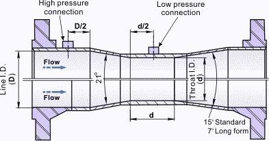
In Figure 2the standard geometry for a venturi is shown. D represents the diameter of the pipe and d represents the diameter at the throat. From the figure it can be seen that the length of the throat is to be the same as the diameter of the throat, this is also true for the inlet section of the venturi. The standard angle for the converging section of the venturi is set at 21°, while the diverging angle can be set at any angle between 7° and 15°, for the purposes of this study the diverging section was set to 7° as this was the same as the geometry used in the test data.

For incompressible flows applying Bernoulli’s equation we get Equation 73

P1+12ρu1-2=P2+12ρu2-2

73

Where P is the static pressure, ρ is the fluid density and u is the mean velocity of the flow. The subscript 1 represents the upstream pressure tap and the subscript 2 represents the downstream pressure tap in the throat of the venturi.

From continuity we get:

Q=14πD2u1=14πd2u1

74

Where Q is the volumetric flowrate, D is the pipe diameter and d is the throat diameter.

By combining Equations 73and74,Equation 75is generated.

Qt=πd2411-β4+2P1-P2ρ

75

Where β is the diameter ratio. This can be represented by Equation 76.

β=dD

76

The volume flowrate calculated by Equation 75is only theoretical, the actual volume flowrate can be calculated by adding a correction factor. This correction factor is known as the discharge coefficient, Cd. This is shown in Equation 77.

Q=Cdπd2411-β4+2P1-P2ρ

77

Where

Cd=QQt

78

The theoretical volumetric flowrate can be re-written as shown in Equation 79.

Qt=AThroat(1-β4)×2∆Pρ

79

By substituting Equation 79intoEquation 78an equation to directly calculate the discharge coefficient can be obtained. This is shown in Equation 80.

Cd=Q(1-β4)×2∆PρAThroat

80

Where

πd24has been simplified to

AThroat, the cross sectional area of the throat and

P1-P2has been simplified to

∆Pas the pressure difference.

Validation of CFD Models

Methodology

The experimental data for the verification of the models has been supplied by Tuv nel, a national standards laboratory. The data taken during the tests is extensive and highly accurate, all of the required information to verify the CFD models has been supplied and has allowed for the creation of highly accurate models to be created within ANSYS.

The CFD models were created and run within the University of Strathclyde computer labs using the available Dell Optiplex 7010 i5 computers which have 8GB of RAM, 2 3.2 GHz processors and a 1TB hard drive.

The 2D models were created in ANSYS Design modeller. Initially the design of the 2D models were based on the ISO standards for venturis, however, the geometry of the venturis that can be created by this method can vary slightly depending on assumptions made whilst reading the standards. Once the engineering drawings of the venturis used in the test data was supplied the geometry of the models could be made as accurately as possible. This had a positive effect as the small changes that were made allowed the models to become more accurate when compared to the test data. The models were created in 2D based in the drawings that were provided. Only half of each of the models was created so that the analysis could be run axisymmetrically when the models would be imported into Fluent. 4D was added to the upstream section of each of the models to ensure that the velocity profiles would be correct by the time that the flow reached the venturi, 8D was also added to the downstream sections of the models as the ISO standards state that a venturi should be installed at least 8D upstream of any features on the pipe such as an elbow.

Once the geometry of each model was complete the geometry was imported into ANSYS’s meshing tool. A mapped mesh was added to the face of the geometry so that the mesh could be set to quadrilaterals. This was done so that the edges of each of the cells within the mesh could be made in such a way that they were perpendicular to the direction of the flow, this ensured that the errors during the computational calculations were kept to a bare minimum. Each face also had an edge sizing applied to it using a number of cells division method. Each wall edge section was matched up to a corresponding section of the axis to ensure that the mapped mesh could still be created, the inlet and outlet were also paired together. A bias was applied to the edge sizing at the inlet and outlet to ensure that the mesh was finest at the domain boundary walls, this is so that the wall shear effect can be accurately computed during the analysis. The density of the mesh was also edited across the axial length of the model, this was done by editing the edge sizings at each region, and the finest regions were the converging section and the throat due to these being the areas of greatest interest for the purposes of this study. The downstream region after the venturi meter was left relatively coarse when compared to the rest of the mesh, this was so that the computational time could be optimised as this region did not affect the results of the CFD with respect to this project. The overall density of the mesh was kept constant throughout all of the models by modifying the edge sizings depending on the geometry. Once the mesh was created named sections were then created within the meshing tool, the axis was labelled “axis”, each section of the wall was selected and named under one named section, “wall”. The inlets and outlets were then named “inlet” and “outlet” respectively. This was done so that when the mesh was read into Fluent the program would automatically recognise each section.

The initial meshes were created with over 100,000 elements in each model, the aspect ratio ranged between 1-20, the element quality ranged from 0.1 to 1, however the areas closest to the walls and within the converging and throat sections were the areas of highest quality. The skewness within the mesh ranged between 0.12-1.3e-10, where 0 corresponds to a high quality and 1 corresponds to bad quality. The orthogonal quality ranged between 0.98-1, where 1 corresponds to high quality. The overall quality of the initial meshes produced were of very high quality, however, due to the high number of elements within the models the computational time was excessive. To counter this the density of the mesh in each model was drastically reduced so that each mesh contained around 40,000 elements. As a result the aspect ratio range changed to 1-26, the range of element quality changed to 0.076-1 but there was a higher distribution of high quality elements. The skewness of the mesh did not change and nor did the orthogonal quality of the mesh. As a result of the changes made to the meshes of each model the computational time was drastically reduced while maintaining the high accuracy of the results produced by fluent, the results varied by up to 0.2% between the two different meshes. This shows that a mesh independent solution was reached while attempting to minimise the computational time involved in the CFD analysis.

Before the mesh could be read into Fluent so that the CFD analysis could be run the test data that would be copied into Fluent had to be selected. The supplied test data was extensive with far too many data points to recreate through CFD analysis, this meant that the data had to be selected. Within the available spreadsheet the data was separated into different levels of accuracy by colour coding. The white data was the most accurate, then the beige data, then the red data was the least accurate data. It was decided that there was enough data in the highest accuracy band and so the only data that would be used to read across into Fluent would be the white data. Even after this decision there were still too many data points to try and run analysis on each one. The data was then filtered further by eliminating data points with very similar Reynolds numbers and ensuring that enough data points were selected so that an accurate representation of the relation between the Cd and the Reynolds number could still be shown. It was also ensured that the highest and lowest Reynolds numbers tested were included in each model so that the largest range of Reynolds numbers possible were analysed.

Once the mesh was completed using ANSYS’s meshing tool and the test data was selected, the meshes were read into Fluent. Every time the mesh was imported into Fluent a mesh check was carried out to ensure that there were no errors while using Fluent. The solver was set to pressure-based, absolute velocity formulation, steady time and 2D axisymmetric. The energy equations were left off as they do not need to be solved simultaneously with momentum and continuity when the flows are incompressible as they are in this instance. The laminar model was used when modelling flows where the Reynolds number did not exceed 2300 in either the throat or the pipe as all flow below this point was assumed to be fully laminar. When the flow passing through the throat did exceed 2300 but the flow within the pipe was below 2300 the transition k-kl-omega model was used. A number of turbulence models, such as k-epsilon and k-omega, were tested within this region as well as the transition SST model. While all of these models would allow their residuals to converge below the desired point of 1e-6 it was found that they were much less accurate when compared to the transition k-kl-omega model. This was despite the fact that the transition-k-kl-omega model would not converge. The k-kl-omega model was used throughout the study as it proved to be more accurate than the other available models within this region and the results also proved to be repeatable. Once the flow in the pipe and the throat exceeded 2300 the k-omega model was then used as this proved to be the most accurate turbulence model, it proved to be as accurate as the transition model within this region whilst reducing the computational time required.

After each run was complete the material properties were adjusted so that the most accurate model possible was run each time. The material properties for both Siptech and Aztec remained fairly constant throughout the test data, however, there were slight alterations in the fluid properties in each test run, so to maintain a high level of accuracy these characteristics, density and viscosity, were changed after each run. The walls were also set to aluminium as in the engineering drawings it stated that the venturi meters were to manufactured from aluminium. The cell zone conditions were altered from solid to fluid to create the fluid domain. The boundary conditions were then set. The named section “axis” was set as the axis for the axisymmetrical analysis. The inlet was set to a velocity inlet with the velocity specification method set to “components”. This allowed the velocity to be set as a constant fully axial velocity, the reference frame was set to absolute. The upstream pressure that was supplied within the test data was also input into the initial gauge pressure. The values of the velocity and gauge pressure were edited between each run. The outlet was set as a pressure outlet with the gauge pressure set to the downstream pressure supplied within the test data. The walls were set to stationary walls with the no slip condition applied.

The pressure-velocity coupling scheme was set to simple as this was deemed to be sufficient for the models that were being run. For the laminar models the spatial discretization gradient was set to least squares cell based, the pressure to second order and the momentum equations to second order upwind. For the transition and turbulent models the settings were the same and the remaining spatial discretization factors were all set to second order upwind. This was done to increase the overall accuracy of the results obtained by each model. The residuals absolute criteria were all changed to 1e-6 to ensure a fully converged solution. Surface monitors were added to analyse key characteristics of the flow, mass flowrate, volume flowrate and pressure monitors were all added. The pressure monitors were placed in the same locations as the pressure tapping for each venturi as indicated within the engineering drawings, to do this lines had to be created as surfaces within Fluent with the local height set for each position.

The models were then initialized from the inlet using standard initialization and the models were run until they converged, or in the transition model’s case for a maximum of 4000 iterations. The pressure difference between the throat and the pipe and the volume flowrate from each run was noted down and logged into an excel spreadsheet so that the Cd and the error between the CFD and test data could be calculated. The volume flowrate was noted as it was noticed that this was similar to the volume flowrate given in the test data but ultimately different, the marginal differences were noted to have an effect of the Cd values obtained and so the volume flowrate from each run was noted.

The Cd values were calculated by using equations Error! Reference source not found., Error! Reference source not found. and Error! Reference source not found.. These equations were programmed into excel so that the time spent doing calculations was kept to a minimum.

The work within this study has been carried out on a CFD programme called Fluent. This CFD solver is a product of ANSYS 17.1 and used the steady state, incompressible flow, Navier–Stokes equations to solve the model.

Before being able to analyse the flow within each of the venturis the models were created in ANSYS design modeller in 2D so that they could be used axisymmetrically within Fluent to save computational time. Each venturi was modelled on their engineering drawings and then a further 8D was added to the end of each venturi to simulate a continuance of the pipe. 8D was used as it is stated within the ISO standards for venturis that there must be a minimum of 8D after a venturi of straight pipe before a bend or any other featured can be introduced.

After the venturis were modelled they were meshed using ANSYS’s meshing tool, the mesh was made as quadrilaterals so that the boundary of each element was perpendicular to the direction of the flow to minimise the error in the calculations. Edge sizing were then added to the inlet and outlet of the venturis with bias towards the wall to ensure that the mesh was finest near the wall, again this was done to minimise the errors in calculation of the flow properties due to effects such as wall shear stress. The original models contained 150,000 elements, however, it was found that the computation time required to complete each model was too long and so the element count was reduced to roughly 40,000. It was found that by doing this the computational time required was reduced significantly without a large drop in accuracy of the results, less than 0.1% difference in the error between the test results and CFD results was noticed between the two different meshes.

Once the meshing was complete the mesh was read into Fluent. Within Fluent two different models were used to run the simulations, the laminar model was used when the Reynolds number within the throat of the venturi was less than 2300, the k-kl-epsilon transition model was used once the Reynolds number became larger than 2300 as it was assumed that the flow was turbulent above 2300 and laminar when below 2300. The CFD was also carried out under pressure-based solvers and set to be solved axisymmetrically. The material properties were changed each time to accommodate for the differing factors that were present when the physical tests were carried out and to account for the change in fluid between Siptech and Aztec. The inlet of the venturi was set to a mass-flow inlet and the outlet set to a pressure outlet, the wall of the venturi was set to wall and the axis was set as axis. The values provided for mass flow and upstream pressure were used at the inlet and the value for the downstream pressure was set at the outlet as the initial gauge pressure. The convergence criteria were set to 1e-6, meaning that the solution had converged when the residuals had all reached 1e-6, however, this proved difficult with the k-kl-epsilon model in the transition region as the solution would not converge. The k-epsilon turbulent model was then used to gain the results at this point as this model would converge throughout the transition region, the results from the turbulent and transition model were then compared and it was found that despite the lack of convergence the transition model was significantly more accurate than the turbulence model within this region. As the results from the transition model were found to be consistent as well as more accurate the decision was made to continue with the use of the k-kl-epsilon model. To calculate the Cd lines were set up on each model where the tappings would be for flow measurement so that the pressures at each point could be measured. From the pressures at the inlet of the venturi and at the throat, along with the fluid data provided it was possible to calculate the Cd using Equation Error! Reference source not found., Equation Error! Reference source not found.and Equation Error! Reference source not found..

Results and Discussion

The standard way to present results of this type is for them to be displayed on a graph with Cd on the y-axis and the Reynolds number on the x-axis as a semi-log graph. This is done as it clearly displays the relation between the Reynolds number of the flow and the resulting Cd obtained from the results, the graph is usually displayed as a semi-log graph as there is usually a very large range of Reynolds numbers being analysed, into the millions of Reynolds numbers. As this study is only looking into the very low Reynolds number region, the highest Reynolds number analysed was 20,000, the results are displayed on a regular graph of Cd vs Reynolds number in the form of dot plots. On the graphs the CFD results will be displayed alongside the experimental data for comparison. From the supplied data, the tests have been completed using two different fluids, Siptech and Aztec, both of these fluids have been used throughout the laminar, transition and turbulent regions and as such there has not been a distinction made between them within the results.

To complete the CFD analysis, three separate venturis were selected each with a different β value and differing geometry as shown below in

Table 1.

Table 1: Venturi Geometry

	β	D (mm)	d (mm)
Venturi 1	0.4	154	61.6
Venturi 2	0.6	102.3	61.4
Venturi 3	0.75	154	115.6

The standard geometry for a venturi can be seen below in Figure 3.

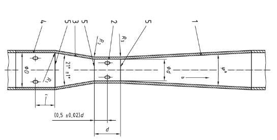
Figure 3: Standard Geometry of a Venturi

From these simple geometry figures and knowledge from the ISO standards it is possible to recreate the venturis in ANSYS. The results from these three different venturi meters can be seen below in Figure 4, Figure 5, Figure 6, Figure 7, Figure 8 andFigure 9. These figures show both the comparison between the test data and the CFD results and the error between the two.

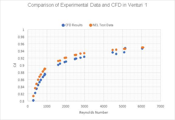
Figure 4: Comparison of Test Data and CFD Data for Venturi 1

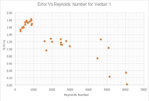
Figure 5: Error Between Test Data and CFD Data for Venturi 1

The results from Figure 4andFigure 5show that the CFD analysis of venturi 1 has been successful. Figure 4 shows the close correlation between the test data and the results obtained through fluent while Figure 5shows a trend in falling error values, as the flow becomes more turbulent and moves away from the transition region the accuracy of the results has increased. There are also two clear regions where there are no results, the first region lies between 1000 and 1500 Reynolds numbers, the second is between 3000 and 4500. This was not desirable, however there were no results available within these regions within the highest level of accuracy bands and it was considered that the general trend of the Cd vs Reynolds number could still be clearly seen.

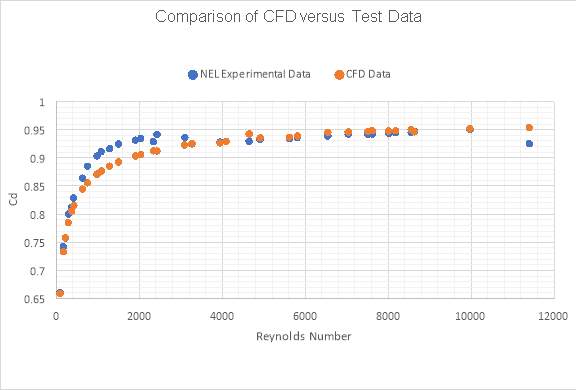
Figure 6: Comparison of Test Data and CFD Data for Venturi 2

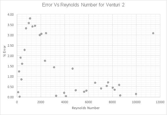
Figure 7: Error Between Test Data and CFD Data for Venturi 2

Figure 6 and Figure 7 show a good level of accuracy of results from the CFD analysis. From Figure 7 it can be seen that the errors vary differently than the errors produced within the model generated from venturi 1. The errors shown in Figure 7 are more representative of the errors that would be expected from the analysis being carried out. The errors in the laminar region begin very small and increase as the model becomes more turbulent. The highest errors then occur within the transition region of the models where the flow through the venturi throat is turbulent but the flow within the pipe remains laminar. The error then falls again as the model becomes turbulent within both the pipe and the venturi throat.

Figure 8: Comparison of Test Data and CFD Data for Venturi 3

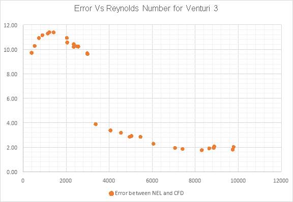
Figure 9:Error Between Test Data and CFD Data for Venturi 3

Despite the test results being used coming from the highest band of accuracy available it has been assumed that there has been an error made while either running or calculating the results obtained from venturi 3. This assumption has been made as the Cd vs Reynolds number curve produced from these results clearly does not follow the general trend of these types of curve for venturi meters. The results appear to have shifted upwards within the laminar and transition regions and as a result the CFD results do not have a close correlation to the test results obtained. However, the CFD results display a curve that is typically representative of what should be expected from a flow meter of this type and since there has been a good level of accuracy obtained from the other two models it has been assumed that the CFD results for venturi 3 show an accurate representation of the flow for a venturi of the same geometry.

A graph containing all of the data plots from the test data for venturi 3 is shown in Figure 10.

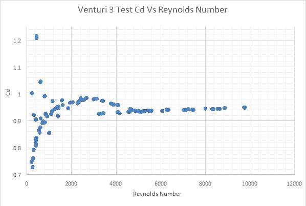
Figure 10: Cd vs Reynolds Number graph for all test data for Venturi 3

Figure 10shows that the graph produced from the test data for venturi 3 shows a curve that resembles the curves produced from orifice plates within the same region of extremely low Reynolds numbers. The graph also shows the high percentage errors that occur in some of the data that has been excluded from the rest of the study. For comparison Figure 11has been shown below.

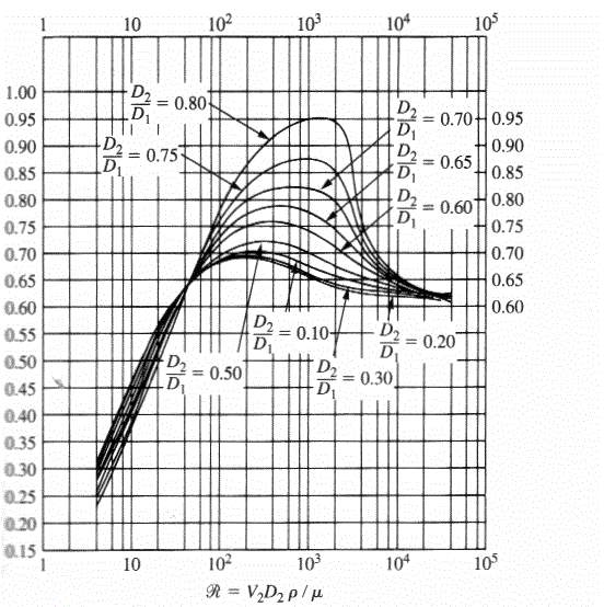
Figure 11: Typical curves for Cd vs Reynolds Number of an Orifice Plate (Ref 10)

It can be seen that the data produced from venturi 3 is not consistent with the data expected from venturi meters.

From the data produced by the CFD analysis it can be said that the levels of accuracy produced are consistently of a satisfactory level, therefore, the models can be said to be verified by the test results. This means that by setting up other models in the same manner the results can be assumed to be accurate, therefore it is acceptable to alter the geometries of the venturi meters and analyse them in the same manner to alter the Cd vs Reynolds number curve.

Modifying The Geometry

Selecting Modifications

From equations Error! Reference source not found., Error! Reference source not found. and Error! Reference source not found. it can be seen that the Cd value varies depending on the geometry of the venturi, the fluid properties and the change in pressure, which in turn depends on the velocity of the flow. Due to these facts, it was decided that the geometry of the venturi should be edited to obtain different measurements of the Cd value. When considering how to alter the venturi meters there was not a lot of areas where change could be made as the geometry of a venturi is relatively simple. The inlet and outlet could not be modified as this would simply alter the size of the flow meter. The throat diameter could not be changed as this would be a change in β of the meter. The converging and diverging sections of the venturi are the only regions where a change could be made without altering the venturi’s β value of the pipe size. The diverging section of a venturi simply allows the flow to ease back to the full pipe diameter and in doing so it reduces the overall pressure loss caused by the differential pressure flow meter. The section that was selected to be modified was the converging section of the venturi, this was also because the largest gradients, such as the velocity and pressure gradients, within the system are present within this region where the flow is being accelerated. The standard converging angle of a venturi meter at this point is 21°, as a change in any other measurement within this region would result in a different β a change in angle was targeted, this would also change the length of this region and thus the length along which the flow can accelerate. The different angles that were selected were 10.5° and 31.5°. These angle were selected as research conducted and published by NEL has considered the effects that these non-standard angles have on venturi meters at higher Reynolds numbers and have had reasonable success with their results. The venturi with an angle of 10.5° was found to be a more stable solution than the standard venturi and the venturi with a set angle of 31.5°.

Methodology

To create the geometry for each of the different venturis the project files were duplicated twice, once for the sharpened convergence angle and once for the eased convergence angle. The duplications were made so that the time required to set up each model was reduced as many of the settings were not required to change.

To modify the geometries of each venturi the design modeler of each duplication was opened. The angles that the converging sections were set to were each changed to either 10.5° or 31.5°. All of the other constraints for the walls remained the same, however, some further alterations were required. The axial section was separated into different regions so that when the mesh was created each section could be selected to align with the corresponding wall section. The lengths of these sections were changed so that the sections all matched up and the mesh could then be created without unnecessary issues.

Once the geometries were complete the project files were updated and ANSYS’s meshing tool was opened. To ensure that the mesh density was kept constant the sizings that were set on each edge were checked. The sizing on the converging section for each venturi was edited so that the density remained constant for each model. The number of divisions was increased for the venturis with eased convergence as the length of the section was increased due to the angle change. The number of divisions was decreased for the venturi with sharpened convergence as the length of this section was decreased due to the sharper angle that was introduced.

The number of elements within the sharpened convergence venturi has been reduced to between 30,000 and 35,000 depending on the model selected. The number of elements within the eased convergence mesh has been increased to 40,000 to 45,000.  The element quality within both of the modified models improved at the lower end of the quality range, both ranging between 0.01 and 1. The distribution of the elements at different element qualities did not seem to differ. The number of elements at the highest quality increased in the eased convergence model while the number of element at the highest quality decreased in the sharpened convergence model, this is to be expected due to the differing number of elements within each model. This shows that the quality of the elements have improved overall.

Figure 12: Eased Convergence Venturi Element Quality

Figure 13: Sharpened Convergence Venturi Element Quality

By looking at Figure 12and Figure 13a comparison can be made between the two mesh qualities. While the overall distribution of elements appears to be the same a large proportion of the extra elements in the eased convergence models appear to be of very high quality.

The aspect ratio and skewness of each model has remain relatively unchanged from the values given in chapter 1. The orthogonal quality of the models did change slightly. Both models retained a maximum quality of 1, however, the lower end of the ranges changed. The eased convergence model had an improved orthogonal quality range of 0.994-1, while the orthogonal quality range for the sharpened convergence model decreased in quality to 0.926-1. This decrease in quality was not significant enough to merit any further alterations to the mesh. From these figures it was decided that the meshes were of high enough quality to proceed with the meshes that were generated.

To finalize the meshes before importing them into Fluent the named sections had to be re-done as they were lost after the alterations to the geometry. This was done in the same was as in chapter 1.

Once the meshes were complete the data to be used for each model was selected. This was done in a similar way to the method described in chapter 1, however, it was decided that less runs were required as these models did not need to be verified and the Cd vs Reynolds number curve could still be produced accurately without as many points.

The models within Fluent were set up in the same way as described in chapter 1 for all regions of flow, laminar, transitional and turbulent. The only difference in the set-up of the fluent models was the positioning of the pressure readings. The line were required to be moved to ensure that they were reading the pressures from the same relative point of the venturi. This was particularly important for the eased convergence venturi as the position of the pressure reading that was read across from the standard venturis would be in the converging section of the venturi, this would drastically affect the results obtained from the CFD. This was still done for the sharpened convergence venturis although it was not as necessary as the previous position of the pressure reading would still be in the pipe section, just slightly farther away as desired, this would only result in minor differences in the pressure reading.

Results and Discussion

The results from the analysis of the modified geometries has been displayed in the same manner as in chapter 1, by a Cd vs Reynolds number dot plot on plain axis.

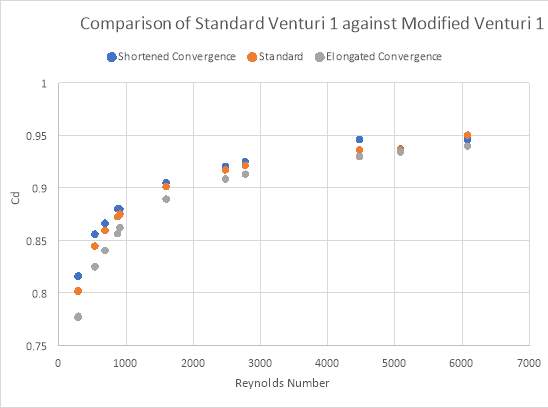
Figure 14: Comparison of Standard Venturi with Edited Venturis

The results shown in the above figure indicate that there is a marginal improvement in the Cd value for the Venturi meter with a converging angle of 31.5°, the lengthened convergence, however, shows a marginal decrease in the Cd values. As the β value for each of these venturi meters remains constant the overall pressure change should remain the same, the slight differences in Cd value may be attributed to the loss of pressure that occurs across any given length of pipe. In the venturi where the convergent region was shortened due to an increased angle the flow must traverse across a smaller distance, therefore, incurring less pressure loss between the two tapping points where the reading would be taken, this would then lead to a slightly reduced overall pressure difference. The opposite could be said for the lengthened convergent region where the overall pressure difference would be increased due to this effect. The larger differences between the meters can be seen within the laminar region, this is where the pressure differences due to this effect would be greatest as there would be a larger wall shear stress, it can also be seen in Figure 14 that as the Reynolds Number increases the difference between the Cd values decreases as the flow becomes more turbulent, thus reducing the wall shear stress and resulting pressure loss.

Conclusions

This study has proven that the effects of Reynolds number on the discharge coefficient of venturi flow meter can be accurately estimated using CFD techniques. The trickiest regions to estimate are the transition regions where the flow is laminar within the main pipe but turbulent within the throat of the venturi, however this can still be calculated to a relative degree of accuracy.

Through the use of CFD it has been demonstrated that some slight changes to a venturi’s geometry can result in a marginal improvement of the discharge coefficient at very low Reynolds numbers, however, the results suggest that within the fully turbulent region these marginal gains may dissipate. In order to fully understand the effects of the changes in geometry further investigation is required.

References

1. Crude Oil, http://www.nasdaq.com/markets/crude-oil.aspx (2017, accessed 13 March 2017)
2. Chapter 2 – Basic Concepts Related to Flowing Water and Measurement, https://www.usbr.gov/tsc/techreferences/mands/wmm/chap02_14.html (accessed 06 April 2017)
3. ISO 5167-4:2003. Measurement of fluid flow by means of pressure differential devices inserted in circular cross-section conduits running full- Part 4: Venturi tubes.
4. Bowman N, The Importance of Correct Measurement. 2017 [Cited 2017 March 1]; Available from: http://classes.myplace.strath.ac.uk/course/view.php?id=11625
5. Hollingshead C.L., Johnson M.C., Barfuss S.L., Spall R.E. Discharge coefficient performance of Venturi, standard concenctric orifice plate, V-cone and wedge flow meters at low Reynolds numbers. Technical Paper, Utah State University, USA, 2011
6. Pal R., Flow of Oil-in-Water Emulsions through Orifice and Venturi Meters. Ind. Eng. Chem. Res. 1993, 32, 1212-1217.
7. Miller G, Pinguet B, Mosknes P, Theuveny B, The Influence of Liquid Viscosity on Multiphase Flow Meters. 8^th International South East Asia Hydrocarbon Flow Measurement, 4^th-6^th March 2009
8. Ishibashi M, Discharge coefficient equation for critical-flow toroidal-throat venturi nozzles covering the boundary-layer transition regime. Flow Measurement and Instrumentation 44 (2015) 107-121
9. Reader-Harris M.J, Brunton W.C, Gibson J.J, Hodges D, Nicholson I.G. Discharge coefficients of Venturi tubes with standard and non-standard convergent angles. Flow Measurement and Instrumentation 12 (2001) 135-145.
10. ANSYS Fluent Theory Guide, Release 15.0, November 2013
11. Experiment No.3: Flow through orifice meter Background and Theory, http://uorepc-nitk.vlabs.ac.in/exp3/index.html (accessed 07 April 2017)