CFD Simulations for Wettability of Different Surfaces
Info: 9254 words (37 pages) Dissertation
Published: 9th Dec 2019
Tagged: EngineeringEarth Sciences
3 Research methods
3.1 Calculation methods
3.1.1 Introduction of Gibbs free energy calculation
Generally speaking, the Gibbs free energy of a multi-phase wetting system [49,50] is calculating by the equation (1):
G= γla Ala + γsl Asl + γsa Asa
(3.1)
where γ is the surface tension, A is the interfacial area. s, l and a stand for solid, liquid and air, respectively. In order to find out the specific expression of the Gibbs free energy, an assumption has been made that the volume of the droplet is very tiny and a constant value is kept. Thus, the effect on the droplet penetrating the grooves can be ignored. What is more, the surface tension drag force and the droplet gravity should also be ignored as they are too small to consider.
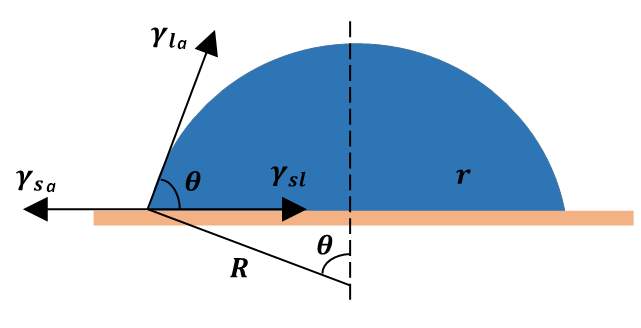
Figure 3.1 Diagram of the wetting system for a droplet.
Based on these assumptions, an interfacial area could be obtained by calculating the outside interface of the droplet and the interface inside the grooves:
Ala = 2Rθ + 2R fla sinθ (3.2)
Where R and θ are the radius of the droplet and original contact angle, respectively. fla stands for the volume fraction that the droplet contacts with the air on the grooves (0 ≤
fla≤ 1). The following equation shows the solid-liquid interfacial area:
Asl = 2R fsl sinθ
(3.3)
Where
fslis the wetting area per unit base area of the droplet (0 ≤
fsl≤ r) and r is the surface roughness ratio. Thus, the solid-air interfacial area can be obtained by the difference between the total solid area, At, and the wetted area:
Asa = At – 2R fsl sinθ (3.4)
The radius of the spherical cap could be calculated by the relationship between the droplet radius and its volume:
r = R sinθ = sinθ [V/(θ – sinθ cosθ)]1/2 (3.5)
Substitution of formulae (2-4) into Eq. (1), a representation of surface Gibbs free energy can be derived:
G = 2 γla (θ+ fla sin θ)[V/(θ- sinθ cosθ)]1/2 –
2 fsl (γsa – γsl) sinθ [V/(θ – sinθ cosθ)]1/2 + At γsa (3.6)
3.1.2 The calculation of Young’s contact angle
Young’s contact angle is derived based on an assumption that the surface is designed to be a perfect flat surface with a roughness. In this case, fsl=1, fla = 0, thus, the Gibbs free energy of Young’s model can be obtained as the Eq. (6).
G = 2 γla θ [V/(θ – sinθ cosθ)]1/2
–
2 (γsa– γsl) sinθ [V/(θ – sinθ cosθ)]1/2 + At γsa (3.7)
It can be seen from Eq. (7) that Gibbs free energy is a function of one variable, contact angle,θ. And a differential equation of Gibbs free energy can be derived as the following equation.
dG/dθ= 2V1/2[γla cosθ – (γsa– γsl)] (θcosθ –sinθ)/(θ– sinθ cosθ)3/2
(3.8)
Eq. (8) shows that when
dG/dθ (θ=θY)equals zero, a theatrical contact angle
cosθY= (γsa– γsl)/γlacan be obtained. This is the famous Young’s equation for the equilibrium contact angle on an ideal surface and it is a foundation to derive the following models of Wenzel and CB contact angle.
3.1.3 The derivation of Wenzel and Cassie-Baxter contact angle
It might be noticed that At can be regarded as zero in Eq. (7-8), because it is a constant value and will not effect to the calculation results of the Gibbs free energy. Another assumption has to be made is that all the contact situation, for example, the interfacial surface inside the pillars and outside should be evaluated as a horizontal value so that surface fractions of
fsland
flacan be derived. To reduce the complexity of the Gibbs free energy calculation, dimensionless Gibbs free energy can be calculated instead, it reduced the difficulty of calculation and the representation is shown below:
G*=G2 γlaV 1/2=θ– sinθ cosθ-1/2(θ– βsinθ)
(3.9)
where
β = fsl cosθY – fla. It is known as Cassie-Baxter (CB) contact angle derived when the minimal Gibbs free energy obtained. Assuming that
dG*/dθ (θ=θCB)equals zero, then the CB contact angle can be derived:
cosθCB= fsl cosθY – fla (3.10)
If the grooves are fully penetrated by the liquid droplet (fsl =r and fla=0), the CB state will be transferred to the Wenzel state and its equation is given as equation (11):
cosθW= r cosθY
(3.11)
After the calculation of two contact angle
θWand
θCB, substitute the value of contact angle into equation (9), two Gibbs free energy of Wenzel and CB state can be obtained respectively. This is a crucial step as it will decide which state the wetting system will be at a steady state by comparing Wenzel and CB Gibbs free energy. More detailed calculation will be given of a specific geometry in next chapter.
3.1.4 Surface modelling
By the derivation of the Gibbs free energy, the theoretical equilibrium contact angle of a liquid droplet can be done on the fabricated flat-top pillars surface and a semi-circular grooves surface model (the flat-top surface is as shown in Fig. 3.1(a). These two surface models are chosen as they are simple geometry but widely found in a natural and artificial situation. For example, the surface geometry of a Lotus leaf can be regarded as a semi-circular grooves structures and flat-top pillars surface are usually selected to manufacture an industrial super-hydrophobic surface.
The unit cell can display all the characteristic dimensions of the whole surface. When a liquid droplet falls onto a surface and remain stable on it, the penetrating depth will be fixed at that time. Because of it, the value of penetrating depth z can be obtained. In a case of flat-top pillars model, a and h represent the width and depth of each pillar. fla can be calculated by the horizontal length exposed to the air and fsl can be derived by the total length solid regions wetted by liquid. The corresponding fractions can be obtained from Eq. (12):
fla = 1 – a fsl(z) = a + 2z (0≤ z < h)
(3.12)
For semi-circular model, an illustration can be seen in Fig. 3.2(b).
rrepresents the radius of semi-circle and z is the penetrating depth, then. fsl and fla can be calculated by the lengths of the wetted solid surfaces as presented in Eq. (13):
fla=2(r-r2-(r-z)2 ) fsl = 2r arccos( r-zz )
(3.13)
By substituting the surface fraction back to contact angle representations, the Gibbs free energy can be derived and the stable situation can be determined by surface energy theory which is the system will tend to be stable when the surface energy approaches to the minimum value. Then, compare the Gibbs free energy of Wenzel and CB state, a steady state can be obtained. The calculation of a specific case will be an inverse way.
These are the default steps to calculate the Gibbs free energy which will be carried out in the next simulations. The calculation normally starts from the characteristic dimensions of a specific surface. In this paper, two geometries of flat-top pillar and semi-circular surface are tested. And the surface properties specification has already given out above. Once the surface properties obtained, i.e. the fraction of multi-phases fsl and fla, the contact angle under two different assumptions (Wenzel model and CB model) can be derived. However, which state will be the steady state is not yet known and the calculation of surface Gibbs free energy is of importance because this is a critical parameter to decide when the system will tend to be stable. After calculating the Gibbs free energy of a specific surface geometry, it can be determined at which state the system will be the most stable and that is where the Gibbs free energy achieves its minimum value.
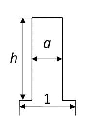
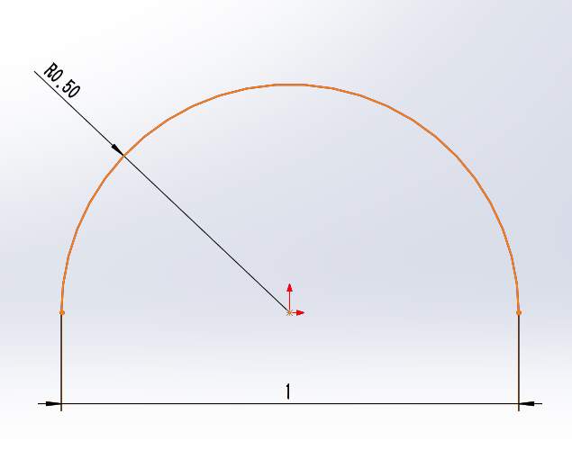
Figure 3.2 an illustration of flat-top pillars geometry and semi-circle
3.2 Simulation methods
All the simulations will be operated on STAR-CCM+, up to now, the physical model has already been determined. Because this is a two-phase situation so that multiphase function will be involved in this project. Multiphase flow is a term which refers to the flow and interaction of several phases within the same system where distinct interfaces exist between the phases. The term ‘phase’ usually refers to the thermodynamic state of the matter: solid, liquid, or gas.
In modelling terms, a phase is defined in broader terms, and can be defined as a quantity of matter within a system that has its own physical properties to distinguish it from other phases within the system. For example: Liquids of different density; Bubbles of different size; Particles of different shapes.
Multiphase flows are different from multi-component flows. In multi-component flows, the varied species are mixed at the molecular level. These species have the same convection velocity. In multiphase flows, the divergent phases are mixed at the macroscopic scale. These phases have different convection velocity. Many flows are multiphase multi-component flows.
3.2.1Establishment of the simulation regions
In this paper, the simulation can be classified into two types. One is the standard Young’s contact angle with no manufactured surface which means the surface in this case is an ideal surface. The other is Wenzel and Cassie-Baxter contact angle with different shaped surfaces which needs to import an external surface with geometric shapes. However, both cases will be carried out under a same fluid region. Fluid region is a region of all the fluids which will participate the simulation. Air and water droplet are the fluids which will be modelled with the region. The size of region should be big enough to be able to simulate the real situation when water droplet falling onto the surface and it should also be small enough because the size of region decides the cell numbers of mesh directly. Normally, more cell numbers got, the CPU time would increase massively so that it is significant to control the size of fluid region properly. There is a balance to be made between the accuracy and CPU time. In this simulation, the final size of fluid region has been set up to a
6mm×6mm×6mmcube which could contain an imported surface with a dimension of
5mm×2mm×5mm. To reduce the modelling time, this 3D fluid region will be converted into 2D region as shown in fig. 3.3.
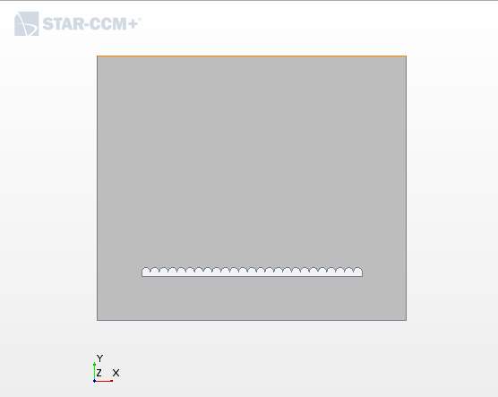
Figure 3.3 the graph of geometry scene in STAR CCM+
For Young’s contact angle simulation, the bottom of fluid region can be treated as target surface and the result can be observed on the bottom surface. For Wenzel and CB contact angle simulation, an imported surface is the target surface which the water droplet will fall on.
The establishment of all the geometry which include the surface and fluid region is the foundation of all simulations because all the simulation processes will happen within the fluid region.
3.2.2Mesh and physical models
Mesh is an ordinary process of CFD software that is a numerical mathematics method to make the research object can be solved. Mesh is the discretized representation of the computational domain, which the physics solvers use to provide a numerical solution.
STAR-CCM+ provides mesher and tools that you can use to generate a quality mesh for various geometries and applications.
STAR-CCM+ could provide the following meshing strategies which are suitable for different situations:
*Unstructured Meshing:
◦Parts-Based Meshing — Parts-based meshing builds the mesh models by the settings of the physics continua and this is a flexible meshing technique. This strategy shows some advantages compared with region-based meshing.
◦Region-Based Meshing — Region-based meshing builds the mesh of the surface and regions based a size of region. And region-based meshing is not available in parts-based meshing, if you want to acquire them both at the same time.
*Structured Meshing:
◦Directed Meshing — Directed meshing normally gained a high-quality, well-structured meshes based on CAD geometry. This meshing is conducted by building a surface mesh guided with a line over the CAD geometry and this surface will sweep throughout the body or a 2D mesh through the volume of a geometry part.
STAR-CCM+ provides both finite volume and finite element solution methods. The finite element approach can be applied when certain requirements are needed for the mesh.
The Parts-based meshing will be used and Parts-based meshing is the main method of all current and future meshing developments in STAR-CCM+. The concepts of the mesh, composites, parts, surfaces, and operations are the main properties of this meshing and they also are the common concepts on CAD and CAE software.
As mentioned before, size of mesh is vital to the efficiency which is so-called CPU time. Besides, less number of mesh grids doesn’t always mean good things to the simulation because accuracy is another important part that must be fulfilled.
There is a way to find a balance between mesh quality and mesh quantity. A mesh grid independency test is a method to examine if the mesh grids are enough to simulation.
In this case, the base size of mesh is set as
10-5 mmand an additional step of mesh refinement is also adopted. Mesh refinement is a process that only concentrating on the target region and ignoring the other non-important regions. The specific operation is keep the global mesh size and establish a higher quality mesh which only appears around the target region, in this case, the target region is the space around the water droplet. The mesh refinement is based on global settings, and an accuracy of 25% of the base size is taken in this simulation which means the absolute mesh size of refinement is
0.25×10⁻⁵ mm. Then, build the mesh with settings above and a three-dimensional meshed cube will be obtained. To reduce the CPU time of the following simulations, current 3D mesh will be converted into 2D mesh, also this step will help us to observe the contact angle better because the geometry and water droplet are axis-symmetric. The final mesh is shown as in figure3.4. It can be easily seen how the mesh refinement works and a clear section view which could contain all the physical information is available within this 2D mesh.
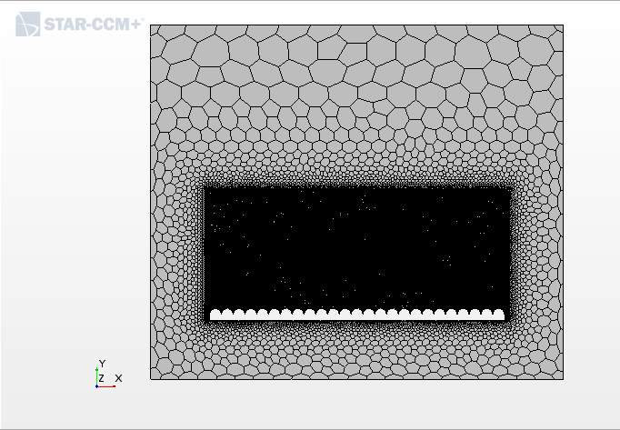
Figure 3.4 The mesh scene in STAR CCM+
Another important setting is the choice of physical model and this will decide if the simulation can reflect the real situation when a water droplet falling onto a surface. The key settings of this part are the selection of Eulerian multiphase and interaction between Eulerian phases. In this case, water and air are two phases involved and the surface tension force has been set to 0.075 N/m which is a factor indicates interaction between two phases. Both Eulerian phases have been selected as constant fluid with their default density and viscosity. The fluid simulation method is VOF method which has been introduced already and fluid type is selected as laminar considering this is a slow and relatively steady case. The other routine settings are shown in the figure 3.5. And they are easy to understand and most of them are required settings and no need to explain in detail.
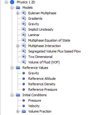
Figure 3.5 Physical settings of modelling
3.2.3 Boundary conditions and solver
Before running the simulation, boundary conditions are the last settings which need to be done. After converting the 3D mesh into 2D mesh, there are 4 boundaries for Young’s model case and 5 boundaries for Wenzel and CB model case with imported surfaces.
For Young’s model, the top surface of fluid region is selected as pressure outlet which means the region is connected to environment so that the pressure is the standard pressure. Two vertical surfaces remain as ‘slip wall’. And for the bottom surface, the boundary condition is selected as ‘non-slip wall’ and the contact angle can be chosen for this surface. Here, different values of contact angle will be selected when running different simulations. For example,
120°is selected during all the simulations of Wenzel and CB model cases.
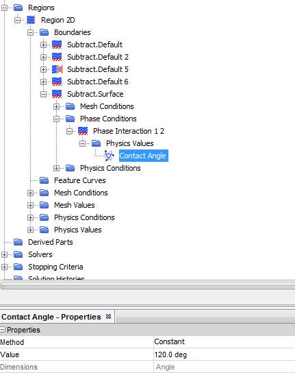
Figure 3.6 the settings of boundary conditions
A specification is need to state is the setting of contact is actually how this CFD software define the properties of a surface. Normally, the surface tension between solid surface and fluid is used to represent the properties of a surface, for example,
γsa and γslin Young’s contact angle equation.
According to the Young’s equation:
γlacosθ= γsa – γsl
Where
γsaand
γslare the interfacial, air-solid and liquid-solid surface tension. So that
cosθ= γsa – γslγla
γla
is the surface tension between air and water which is checked from the table and this value is 0.072 N/m. In STAR-CCM+, both contact angle and
γla(surface tension) can be assigned which means the other two surface tension values
γsl and γsacan be derived based on equation above. That is how the roughness and properties of the surface can be controlled in STAR-CCM+.
After finishing the settings of boundary conditions, it is ready to run the simulation and one more step to be taken is the settings of solver. The number of iterations and inner steps will decide the modelling time of a simulation, also, a scalar scene is needed to observe some physical parameters, for example, the density of air and water, volume fraction of two fluids involved in this simulation and the velocity of air and water during the process of falling.
To evaluate the results more accurately, the setting of 5000 iterations with 2 inner steps which means 10000 physical steps is selected. Two scalar scenes of density and volume fraction are established.
Up to now, all the settings are finished and the simulation is ready to run. Specific values are required with different research purpose and the discussion of results will be introduced in next chapter.
4 CFD simulation results
To simulate a hydrophobic surface and water droplet behaviour, a suitable CFD software should be chosen for this task. Star CCM+ with powerful functions is adopted in this project. By using STAR CCM+, a CFD software with powerful functions based on the solution of Naiver-stokes equation the wetting behaviour can be simulated with a method of VOF model.
Before the simulation, there are a few specifications that need to be cleared out. The basic modelling method of this project is VOF method which is a method of multiphase condition. The main point of this method is to determine the type of fluids and the interaction between them. In this project, two fluid phases are air and water both with a constant density. The surface tension between two phases is 0.072 N/m which is checked from the table of surface tension between air and water.
The simulation will start from the Young’s contact angle simulation to justify the reliability of the physical model. After that, simulation with different types of manufactured surface will be taken into consideration and this project will classify this situation into two categories which is known as Wenzel and Cassie-Baxter model.
4.1 Young’s contact angle
4.1.1 Specification of Young’s contact angle
When modelling Young’s contact angle, the surface is assumed as an ideal surface with no geometric features on the surface. But it doesn’t mean this surface has no roughness. The roughness of surface is represented in a way of contact angle or it can be called wettability. As mentioned in chapter 3, the roughness properties are controlled by simply giving values to contact angle in simulation settings. The contact angle in STAR CCM+ is actually the Young’s contact angle, and measuring the results of Young’s contact angle case and check if it is the same as the value assigned before, then the model of Young’s contact angle can be proved to be correct or not.
4.1.2 Results
So that the equilibrium contact angle is the only value which is to be assigned, Serval types of contact angle, the value will be set as
90°,
120°and
180°.
1.Young’s contact angle of
90°
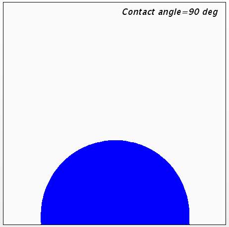
Figure 4.1 the result of CA=
90°
A contact angle of
90°can be observed in figure 4.1,
90°is a criterion of hydrophilic and hydrophobic surfaces, if this angle is bigger than
90°, the surface would be hydrophobic as introduced before.
2. Young’s contact angle of
120°
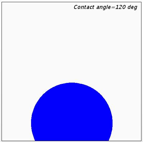
Figure 4.2 the result of CA=
120°
When contact angle comes to
120°, the surface has already become hydrophobic and the water droplet beads on the surface as seen from figure 4.2. By measuring the contact angle, this value is
120°as assigned.
3. Young’s contact angle of
180°
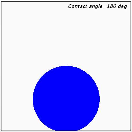
Figure 4.3 the result of CA=
180°
The contact angle of
180°doesn’t exist, however, it can be obtained theoretically to testify if the physical model of simulation is correct. The expected result is that water droplet totally stands on the surface with little contact area. Due to the influence of gravity, surface tension and other factors, the result shows the water droplet beads on the surface with a minimal area which gives a contact angle >
170°.
4.1.3 Summary
The results of Young’s contact angle show that the physical model of this simulation is correct, the contact angle can be obtained accurately as designed. Due to this, the following simulation can be continued when the surfaces come to more complex geometries instead of an ideal surface. This is the foundation of the further simulations and it is also the basic situation as both Wenzel and CB contact angle are derived based on the Young’s contact angle.
A conclusion can be found is the surface properties such as roughness and surface tension are shown in the way of contact angle in this CFD software. The only setting required is to assign value to contact angle under the boundary conditions of the target surface and to see if the final results are corresponding to the desired results.
After obtaining the Young’s contact angle, the Cassie-Baxter and Wenzel contact angle can be derived with equations respectively. And influences of different geometries and steady state models will be discussed during next sections. Normally, the characteristics of manufactured wetting surface will influence the contact angle, i.e. the contact angle of an ideal surface would be Young’s contact angle as shown in this part. However, the contact angle will be different when the surface has some geometric shapes and the final contact angle will not be the Young’s contact angle anymore. Instead, the other types of contact angle models will be applied to specific conditions and it will be discussed later.
4.2 Flat-top pillar geometry
The geometry of flat-top pillar is shown as in figure 3.2. The surface is consisted of a certain number of pillars and an illustration of a unit pillar is shown below. The characteristics of this kind of surface will be determined by the dimensions of width a and depth h. In this part, the purpose of simulation is to specify the relationship between contact angle and different geometric dimensions. The influence of the change of geometry and how it will affect the wettability behaviour. Both Gibbs free energy theorem and contact angle model will be considered in this part.
The drawing of flat-top pillar surface is carried out by using Solidworks, the length of surface board is
5 mm.
4.2.1 Criteria calculation
A.
h
is a costant
I. the surface fraction
fsl and fla
With the geometry of flat pillar, a and h are the width and depth of each pillar and two situations of different variable values will be simulated in this project.
First, keep the depth
ha constant value=0.1 and
ais changing within the range of (0, 0.2), here 0.2 is the length of a unit pillar as shown in the figure 3.2.
In this case,
flacan be calculated by the length of the horizontal line exposed to the air and
fslwas calculated by the total length solid section that was wetted by liquid. The corresponding values can be obtained.
fla = 0.2 –a fsl(z) = a + 2z (0≤ z < h)
II. Wenzel and CB contact angle
By using the terms above, the Wenzel and CB contact angle can be derived first which is the only variable when calculating the Gibbs free energy. The representations of Wenzel and CB contact angle are
cosθCB= fsl cosθY – flaand
cosθW= r cosθYrespectively. In this case, depth
his a constant value and width
ais changing, so that
θCBwill change with width
aand
θWwill remain a constant value because the surface roughness
r=0.2+2hand this is a constant because
hdoesn’t change. Here,
0<a≤0.2 mm, 0≤ z < 0.1mm, then substitute the contact angle into the equation of Gibbs free energy and obtain the graph of Gibbs free energy vs
θCBwhich is determine by width
aand penetrating depth
z. To plot the graph with a better illustration, a definition of relative penetrating depth z* will be introduce here. The relative penetrating depth z*=z/h and
0≤z*≤1. Based on this definition, the system will be in Wenzel state when z*=1. The fraction equation can be rewritten as
fla = 0.2 –a fsl(z) = a + 2z*×h (0≤ z < h)
III. Gibbs free energy
The representation of Gibbs free energy is
G*=G2 γlaV 1/2=θ– sinθ cosθ-1/2(θ– βsinθ)
Here,
β= fsl cosθY – fla. It is well-known that Cassie-Baxter (CB) contact angle
θcould be derived when the minimal Gibbs free energy can be fulfilled.
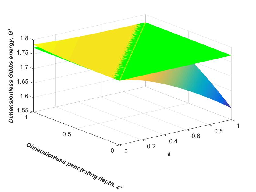
Figure 4.4 the dimensionless Gibbs energy plot in 3D
It can be found that with the change of width
aand penetrating depth
z, the Gibbs free energy of Wenzel state is higher than that of CB state at most time and when penetrating depth
z=0, Wenzel Gibbs energy is greater than CB Gibbs energy, which means, when the system is in a stable stage, the wetting state will be CB state instead of Wenzel state as CB state has a smaller Gibbs free energy in this case. Based on the surface energy theorem, all the states will maintain the lowest surface free energy, so that the Wenzel state won’t be stable in this situation.
VI. transition point between Wenzel and CB state
For a specific case in which the width
ahas already been determined, a 2D graph of Gibbs free energy and relative penetrating depth can be plotted as shown in figure 4.5. It can be found that the Gibbs free energy will change when relative penetrating depth z* is less than 1 and it will become a point value when z*=1. This point is the Gibbs free energy when the system is in Wenzel state and the values when
0≤z*<1indicates the system is in CB state. The stable point can be obtained by comparing the value of Wenzel Gibbs free energy and CB Gibbs free energy too. As said before, the Gibbs free energy of Wenzel state is higher than that of CB state in 3D plot so that it is the same result in this 2D graph.
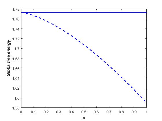
Wenzel
CB
Figure 4.5 Gibbs free energy with width
a
in 2D
For every single value of a, there exists a stable state with the minimum Gibbs free energy and it can be either Wenzel state or CB state. Each stable Gibbs free energy has a corresponding contact angle and this contact angle is a function of specific width
afor a determined geometry. Then plot the relationship between width
aand contact angle in steady state as shown in figure 4.6. A ‘transition point’ can be derived which is a criterion of contact angle in steady state.
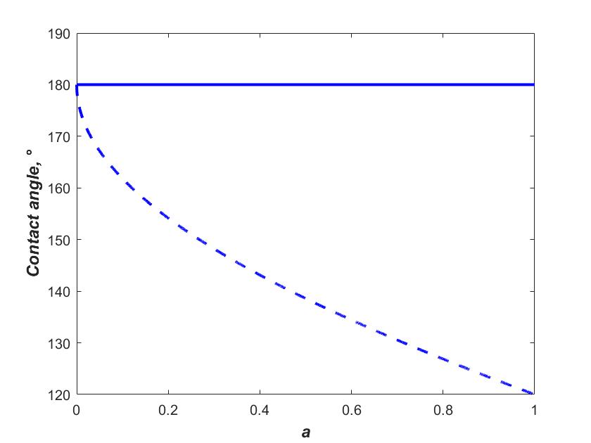
Wenzel
CB
Figure 4.6 Contact angle of Wenzel and CB state
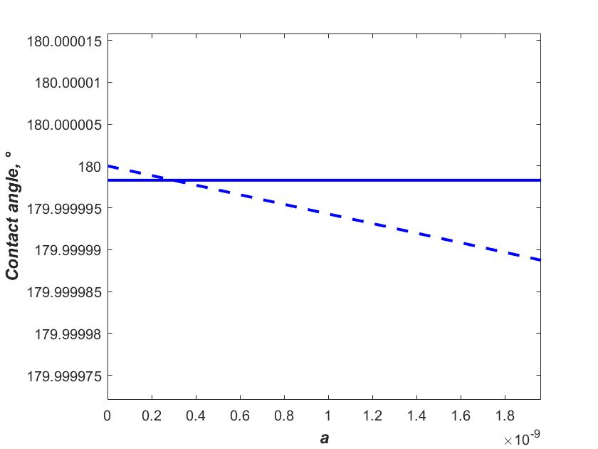
Wenzel
CB
Figure 4.7 the transition point in a zoomed view
With the increasing of width
a, Wenzel contact angle
θWremains a constant and CB contact angle
θCBdecreases with
a. A intersect is found when
a=0.2in the fig.4.7 and it is the transition point when a unit cell is applied. However, The Gibbs free energy calculation shows that the steady state should always be in CB state in real situation which means no transition point should be found. Actually, if substitute this
a=0.2of a unit cell into the real dimension that the total length is
0.2 mm, the corresponding transition value will be
0.2×0.2=0.04 mmand this value can be ignored as it is too small to be considered for the simulation. Same idea that calculating the transition point by using a ratio of a unit cell will be used later.
The following simulation results should show that with the variation of width
a, the water droplet will remain standing on the surface and will not fill up the grooves fully. Three situations will be tested with different values of
a. As the transition point or critical value of this case can be ignored so that it can be regarded as there is no transition point under this situation. Three random values of width
awill be assigned to see if the results are coincidence with the theoretical assumption. What should be observed is the water droplet standing on the surface of flat-top pillar and all the pillars won’t be filled up with water fully. Then the conclusion that CB state will be the final steady state can be obtained in this case. Furthermore, the contact angle at the final moment will be the CB contact angle which can be calculated by equation (10).
The second situation considered for flat-top pillar is keeping the width
aa constant value and assigning different values to the depth
h. The width
ais set as
0.1 mmand three different values of
0.1 mm, 0.05 mmand
0.04 mmwill be assigned to the depth
h. Unlike the previous situation, these values are not chosen randomly because there exists a critical point that will separate Wenzel state and CB state or it can be called ‘transition point’.
B.
a
is a constant
In this case,
flacan be calculated by the length of the horizontal line exposed to the air and
fslwas calculated by the total length solid section that was wetted by liquid. The corresponding values can be obtained.
fla=0.2-a=0.1 fsl(z) = 0.1+2z (0≤ z < h)
It is obvious that
fsl and fslis a function of z only once the width
ahas been assigned as a constant. However, the h is changing in this case and it will influence the value of z because the range of z is determined by h. If rewrite the equation of fraction, it will be
fla=0.2-a=0.1 fsl(z) = 0.1+2z* ×h (0≤ z < h)
II. Wenzel and CB contact angle
It is clear that
fslis determined by the value of z*
×hand the CB contact angle can be derived with it. Knowing width
a=0.1 mmand
0≤h≤0.2 mm, the CB contact angle is represented as
cosθCB= fsl cosθY – fla
Where
θYis the Young’s contact angle and it can be found that
cosθCBis a function of relative penetrating depth
z*and depth
h.
The Wenzel contact angle is calculated by
cosθW= r cosθY, here r is the surface roughness which is
0.2+2hin this case. Unlike the previous situation, the value of
θWwill change as the depth
his changing.
III. Gibbs free energy
The calculation process is similar with the first part, the Gibbs free energy will be derived first. As mentioned above, the equation of Gibbs free energy is
G*=G2 γlaV 1/2=θ– sinθ cosθ-1/2(θ– βsinθ)
Gibbs free energy is a function of
cosθCBand
θCBso that the relationship between Gibbs free energy and relative penetrating depth
z* and depth
hcan be plotted as shown in figure 4.8. It can be found that two surfaces are intersected when the variable are changing. If the depth
hhas already chosen for a specific case. Then the relationship between Gibbs free energy and relative penetrating depth z* can be plotted. It is a 2D graph when choosing different value of h, with the change of relative penetrating depth z*, the Gibbs free energy will vary with it and reach a minimum value which is the stable point. And the Gibbs free energy of Wenzel state is determined when z*=1 as before. By comparing the Gibbs energy values of Wenzel and CB state, a steady state can be found.
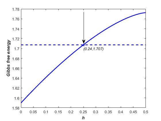
figure 4.8 the Gibbs free energy plot with depth
h
VI. transition point between Wenzel and CB state
Similarly, for every single value of h, there exists a stable state with the minimum Gibbs free energy and it can be either Wenzel state or CB state. Each stable Gibbs free energy has a corresponding contact angle and this contact angle is a function of specific width a for a determined geometry. Plot the relationship between width a and contact angle in steady state as shown in figure 4.9. A ‘transition point’ can be derived which is a criterion of contact angle in steady state.
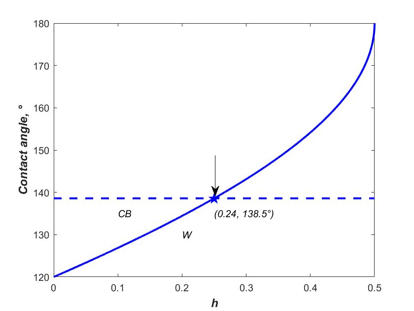
Figure 4.9 the contact angle of Wenzel and CB state
With the increasing of h, the CB contact angle remains a constant because this is the steady state assuming that system is in CB state and when z*=0 is the most stable case. The Wenzel contact angle rises when h is increasing. An intersection is obtained where two lines come across. This intersection point is a transition point which means the contact angle of Wenzel and CB state are same when h=0.048. The graph above is plotted with a standard unit cell. The illustration of a unit cell has been given before. The transition point of a unit cell is where depth
h=0.24and the transition point of this geometry can be obtained by
0.2×0.24=0.048with a same ratio of a unit cell.
Beyond this point, Wenzel contact angle will be bigger than CB contact angle and the steady state of the wetting system will be in CB state at that time. If
h<0.048, Wenzel contact angle will be smaller than CB contact angle and the steady state of the wetting system will be in Wenzel state instead.
The following simulations should be carried out focusing on this critical value h=0.048, so that different values of
0.1 mm, 0.05 mmand
0.04 mmwill be assigned to the depth
hto see if there will be a transition of state when the simulation running with these geometries. The results of h=0.1 and 0.05 should be similar is that water droplet will stand on the pillars and the final state is CB state. The result of h=0.04 should be different that water droplet penetrates all the pillars and the final state is in Wenzel state.
4.2.2 Simulation results
All the simulations run with a same Young’s contact angle of
120°and under the same model of simulation. The only difference is the surfaces with different size of geometries.
A)
h=0.1, a=0.02
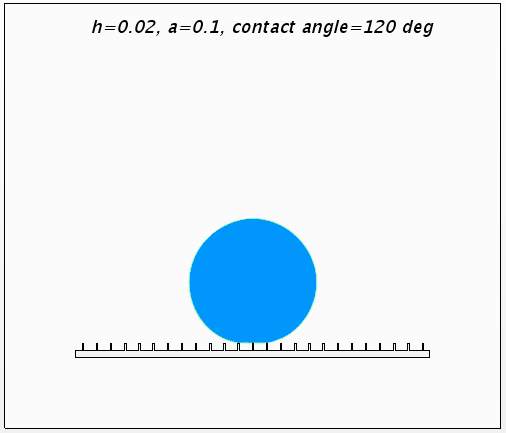
Figure 4.10 the results of
h=0.1, a=0.02
This is the result when
h=0.1, a=0.02. Based on the calculation before, the steady state should be in CB state. It is clear that water droplet is standing on the surface and extra water penetrates into the pillars so that it is sure that this wetting system is in CB state with this geometry.
The contact angle is measured to be around
140°and Young’s contact angle which is equilibrium contact angle is assigned as
120°. It can be found that surface wettability has been influenced with this flat-top pillar geometry. And the surface becomes more hydrophobic than before as the contact angle increases from
120°to
140°.
As the system is in CB state, this contact angle can be also calculated with the equation:
cosθCB= fsl cosθY – fla
B)
h=0.1, a=0.05
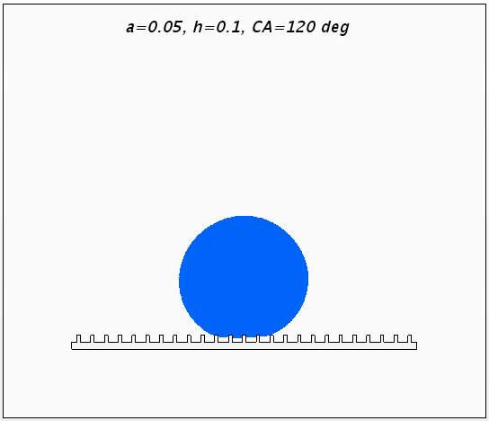
Figure 4.11 the results of
h=0.1, a=0.05
This is the result of )
h=0.1, a=0.05. The final state should be the same as before according to the calculation. And water droplet remains standing on the surface and a little amount of water flows into the pillars but the system is still in CB state with no doubt. It is noticeable that the penetrating depth is not 0 in this case and it is different from the theoretic hypothesis. This can be caused by some reasons, one is that the simulation doesn’t run with enough time which means the system is not in steady state yet. Also, the calculation doesn’t take all the physical factors into considerations, like fluid type, laminar or turbulence, influence of gravity and the interaction between air and water. These could affect the result and this might explain the reason why the result doesn’t satisfy the assumption.
However, the contact angle of
137°is still measured which is greater than the original contact angle
120°. The hydrophobicity has been increased compared to the Young’s model surface.
C)
h=0.1, a=0.1
(Standard-pillar geometry)
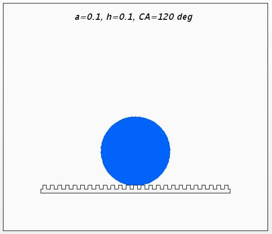
Figure 4.12 the results of
h=0.1, a=0.1
This is the result of
h=0.1, a=0.1and this can be also called the standard because width
aamd depth
hare the same value in this case. The final state should be under CB state too as there is no Wenzel state when width
avaries. It is obvious that no water penetrates the pillars and water droplet only contact with the top surface of flat-top pillars. This result satisfies with the calculation that steady state will occur when penetrating depth is zero.
The simulations of three situations when width
ais changing are finished by now and results are the same as expected before running the simulations. None of these simulation results obtains a Wenzel state when choosing different values of width
a.
After this, two more simulations will be carried out based on this standard-pillar geometry. The width
awill remain a constant and depth
hwill vary to see if it will influence the final results.
A contact angle around
150°is obtained which shows a good hydrophobicity of this manufactured surface.
D)
a=0.1, h=0.05
(
>critical value
)

Figure 4.13 the results of
h=0.05, a=0.1
This is the result of
a=0.1, h=0.05and the depth
his bigger than critical value of
h=0.048. According to the calculation, the Gibbs free energy of Wenzel state is higher than that of CB state when
h=0.05so that the system will be in CB state at the end. As seen from the graph, water droplet is on the surface with a little contact area with flat-top pillars and it is the CB state still though the penetrating depth is greater than before. Same situation has happened in case (b) and the possible reasons have already been discussed before.
The contact angle in this case is also greater than
120°and reaches around
140°.
E)
a=0.1, h=0.04
(h*=0.048,
<critical value
)
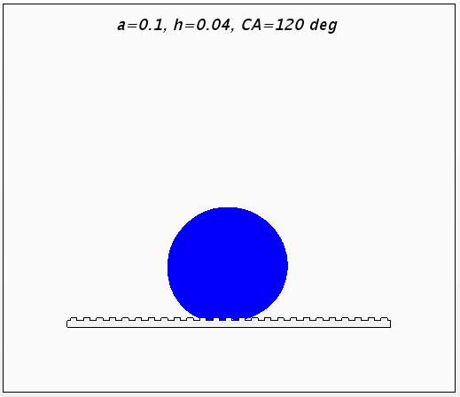
Figure 4.14 the results of
h=0.04, a=0.1
This is the results of
a=0.1, h=0.04and it is a special situation because the depth
his under the critical value which means the phenomenon will be different. The result shows that water droplet penetrates the pillars fully and it is in Wenzel state. The critical value of depth
his 0.048 so that this result is correct based on the calculation.
In this particular case, the contact angle reaches up to 135 approximately. The surface in Wenzel state shows a good hydrophobicity as well as those in CB state.
4.2.3 Summary
After the analysis of these five simulations under different situations, some conclusions and discussion can be made.
1. all the surfaces with flat-top pillar geometry show a good hydrophobicity compared to the original surfaces which means the ‘ideal surface’ in Young’s case.
2. the hydrophobicity of each surface is different and the geometric dimensions are the key factors which caused these results. Also, it is significant to determine the steady state of a hydrophobic surface even though it is hydrophobic already. The dimensions of pillars will influence the steady state as well.
3. there might have some unexpected results which is not compatible with the calculations, but it is acceptable. In a real simulation, for example, in this paper, STAR CCM+ is used for modelling the wettability of a surface. Many settings for this fluid software only are needed which may not be involved in calculations. The settings of Eulerian multiphases and VOF model are the main steps of the simulation, properties of water and air, like density, viscosity, gravity and surface tension force are needed. But they will not be considered in calculations of contact angle.
4. the physical size of simulation in flat-top pillar case is quite small. It is enough to finish the modelling work though it might also influence the precision of the simulation. Normally, the region size should be big enough to avoid some unnecessary problems like the effect of wall boundaries or the effects of eddy within a small region. Considering the state of two fluids, air and water are very stable and they are defined as laminar, so that the small size of region can be acceptable. However, large scale of simulation region should be carried out if possible. Constricted by the CPU limit and experimental time, the simulations in this part are the most accuracy ones as possible.
5. for a flat-top pillar geometry, the width
aand depth
hare main dimensions which decide the hydrophobicity and steady state of a wetting system. It is proved that with a fat-top pillars the surface will have a good hydrophobic behaviour and this kind of surface is easy to manufacture in industry.
4.3 Semi-circular geometry
Besides the flat-top pillar surface, the semi-circular surface may have a different wetting behaviour as its special geometric shape. The semi-circular surface consists of many aligned semi circles as shown in the figure 4.15. A unit cell of semi-circular geometry is represented and it can be found the radius is the main characteristic dimension which decide the surface property. Similarly, the conception of penetrating depth z* will be introduced to this semi-circular geometry to calculate and plot the relationship between the Gibbs free energy and surface dimensions.
4.3.1 Criteria calculation
with the geometry of semi-circular surface, radius
ris the only dimension of this geometry. And different values of radius will be assigned to find out the influence of this value. It is similar with the process before, calculation should start with fractions of two fluids. Then, calculate the theoretical contact angle of Wenzel and CB state. Finally, substitute contact angle the equation of Gibbs free energy and plot the relationship between radius and Gibbs free energy.
I. the surface fraction
fsl and fla
In this case,
flacan be calculated by the length of the horizontal line exposed to the air.
fslis calculated by the total length solid section that was wetted by liquid and it is a curved line in this case. The corresponding values can be obtained.
fla=2r-2rcosθ=2(r-rcosθ) fsl = 2∙r∙θ
Here,
=arccosr-zz, so that the terms above can be rewritten as
fla=2(r-r2-(r-z)2 ) fsl = 2r arccos( r-zr )
II. Wenzel and CB contact angle
the CB contact angle is represented as
cosθCB= fslcosθY – fla
and Wenzel contact is calculated by
cosθW= rcosθY
In this case, surface roughness is
πrwhich is the half length of a circle when the water droplet penetrating the grooves fully.
iii. Gibbs free energy
With the values of Wenzel and CB contact angle, substitute them into the equation of Gibbs free energy
G*=G2 γlaV 1/2=θ– sinθ cosθ-1/2(θ– βsinθ)
A graph of Gibbs free energy of circular surface can be plotted as shown below. It can be found that the Gibbs free energy of CB state is always higher than that of Wenzel state. A same conclusion can be made is that the steady state of this circular geometry will be Wenzel state no matter how radius changes.
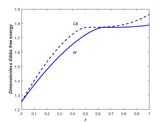
Figure 4.16 the Gibbs energy vs. radius R
VI. transition point between Wenzel and CB state
As the steady state has been proved to Wenzel state based on the plot of Gibbs free energy, which means there is no transition point in this case. If plot the graph of contact angle as shown in figure 4.17. It can be found that CB contact angle is greater than Wenzel contact angle.
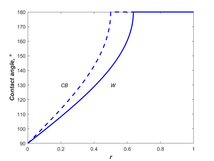
Figure 4.17 the contact angle vs. radius R
4.3.2 Simulation results
a) r=0.1 mm
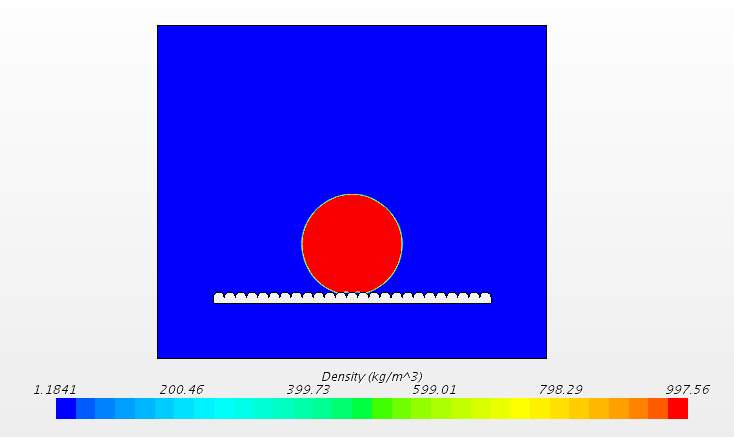
Figure 4.18 the result of a semi-circular surface with a radius of
0.1 mm
This is the result when
r=0.1 mmand it can be seen that the water is penetrating the grooves. As the limit of computer memory, the final state can be obtained for circular geometry. However, a trend that water will keep penetrating can be predicted from the residual plot. The result doesn’t achieve a convergence which means this is not the final state. As the steady state can be determined, more attentions can be paid to the contact angle instead. The original contact angle is
120°, and it reaches to around
145°now with the circular geometry. It also shows a good hydrophobicity.
4.3.3 Summary
With the geometry of circular grooves, two simulations of different values of radius have been finished in this part. The results can reflect the real situation that water droplet falling onto a surface with circular grooves and are acceptable though they didn’t reach the steady state. Some conclusions and discussion can be summarized here:
The geometry of circular grooves is a good choice to obtain a hydrophobic surface as it shows a great wettability behaviour in the simulation results.
It is more difficult to simulate this kind of geometry compared to flat-top pillars. The curve is not only hard to manufacture in industry, it is also not easy to be modelling in STAR CCM+. The requirement of mesh quality is very high and more CPU time is needed for this geometry if a steady state is required.
However, the calculation is rather easy compared with flat-top pillars, because there is only one key dimension ‘radius’ to be assigned. It reduced the calculation work a lot.
5 Conclusions
In this paper, CFD simulations about wettability of different surfaces are carried out and many useful conclusions are derived.
As this is the first time to simulate the wettability behaviour of a surface on STAR CCM|+, this can be an instructional start for the researched in the future. The physical models and settings are proved to be correct by analysing the results. The simulation of Young’s contact angle case is quite successful and it is of significance to this kind of simulations as it is the fundamental situation for wettability behaviour researches.
The theoretic calculations before the simulation are vital to this paper. Derivations of surface fraction, Wenzel and CB contact angle and Gibbs free energy are the key to evaluate the steady state of a wetting system and they are the criteria of measuring a proper contact angle. The calculations are based on the unit cell with a dimensionless scale. The specific situation will be derived by taking a ratio of geometry dimensions. For example, in flat-top pillars case, the calculation is derived assuming that the total length of a pillar is 1 without unit. The real case is that the total length of a pillar is
0.2 mm. A factor of
1/0.2=5can be obtained and it can be used to derive the other physical quantities or critical number.
The surface modelling following the Young’s contact angle is a specific case modelling with a determined surface geometry. In this paper, flat-top pillars and circular grooves are chosen to be simulated and the corresponding conclusions have been made already. The modelling results of these two geometries prove that the settings of STAR CCM+ are correct and the other kind of geometries can be also applied to this simulation program if needed in the future.
There are some problems with the modelling results and most of them are caused by the limitation of computer memory and CPU ability. Actually, the original design is to simulate this wetting system in a 3D region scene. However, the number of mesh cells tends to be too huge to be carried out and a 2D scheme is finally adopted.
Also, during the simulation of circular grooves surfaces, a steady state cannot be obtained because of computer memories are ran out. The conclusion is that a balance between CPU time and precision of modelling is always required and many factors have to be ignored when considering it. Maybe a better design of fluid region can be made in the future to help dealing with problems in this paper with the same computers.
Two geometries in this paper are able to improve the hydrophobicity of a surface and even make it a super-hydrophobic surface. The results showed that the contact angle hysteresis reduced when the modelling surface becomes more hydrophobic. And the flat-top pillars geometry shows a better ability to do that. The other geometries like sinusoidal surface or combination of flat-top pillars and circular grooves may also be able to improve the hydrophobicity of a surface. The simulations of these surface can be operated in the future.
The hydrophobicity is easily effected by the surface geometry and many possible schemes can be operated to achieve high hydrophobicity in industry. The simulations could help engineers to modelling the situations before the manufacture and the results will be helpful to modify the surface.
Besides the simulations of the other types of surfaces, more future works about optimizing the simulations in this paper can be done. First, as mentioned before, different design of a fluid region is necessary if a better result is needed and it is possible to obtain the results in a 3D scene with a good fluid region. Then, more works can be focused on some details of settings. For example, the VOF is the numerical method chosen for this paper. Actually, many other numerical methods like LES, RANS can be chosen too. The solution method is very important as it decides the way how to approach the real solutions. At the end, larger size of simulations is necessary if possible. It is a good idea to optimize the current simulation with a better design, but a more direct solution is to be modelling on a better computer. Without the constraint of CPU, more accuracy and larger fluid region and solutions can be derived. More useful conclusion can be achieved with no doubt.
Cite This Work
To export a reference to this article please select a referencing stye below:
Related Services
View all


Related Content
All TagsContent relating to: "Earth Sciences"
Earth Sciences is a field of study that focuses on the science behind planet Earth. Earth Sciences explores the physical and chemical aspects of not only planet Earth, but it's atmosphere too.
Related Articles

DMCA / Removal Request
If you are the original writer of this dissertation and no longer wish to have your work published on the UKDiss.com website then please: