A CFD Study of Flow Through a Micro – Orifice at High Reynolds Number

Info: 10003 words (40 pages) Dissertation
Published: 17th Jan 2022

Share this: Facebook Twitter Reddit LinkedIn WhatsApp

Abstract

The following study looks into the study of flow through a micro orifice at high Reynolds number with different turbulence models using computational fluid dynamics. The study done was validated with an experiment done on micro orifices previously. The micro orifices were 300μm in diameter and 1mm thick. The Reynolds numbers used in the orifice were fully in the turbulent regime and ranged from 100,000 – 220,000. The original experiment was done with water at 12MPa and 503K. The properties of the experiment were adapted to the simulations and simulations were carried out to see which best describes the flow in and around the orifice. Contour plots showed the pressure reducing in the orifice while the velocity increased and the volumetric flow rate having a quadratic relationship with the pressure. The dimensionless pressure drop across the orifice was found to relatively stay constant which is in disagreement with the experimental results.

Click to expand Contents

Introduction 7

The Experiment 13

Methodology 14

Geometry 14

Mesh Sensitivity Study 16

Setup and Boundary Conditions 19

Governing Equations and Turbulence Models 23

k-ε Realizable Turbulence Model 24

Standard k-ω Turbulence Model 25

Spalart-Allmaras Turbulence Model 25

k-kl-ω Transition Turbulence Model 26

Results 27

Discussion 35

Velocity Contours 35

Pressure Contours 35

Volumetric Flow Rate and Pressure 36

Dimensionless Pressure Drop 36

Conclusion 38

References 39

Figures

Schematic of test section used in Cioncolini et al., (2017) 13

Schematic view of geometry 14

Schematic view of geometry with dimensions 15

Geometry in ANSYS 15

Orifice section of geometry 15

Edge divisions on inlet, outlet and pipe walls 16

Biased edges leading to orifice 17

Orifice inlet, outlet and wall edge sizing 17

Mesh used for analysis 17

Orifice mesh 18

Mesh sensitivity study results 19

FLUENT Launcher 19

FLUENT General task page 20

Convergence history of the k-ε model 22

Convergence history of the k-ω model 22

Convergence history of the Spalart-Allmaras model 23

Convergence history of the k-kl-ω model 23

k-ε velocity contour. Re=100,000 27

k-ω velocity contour. Re=100,000 27

Spalart-Allmaras velocity contour. Re=100,000 28

k-kl-ω velocity contour. Re=100,000 28

k-ε pressure contour. Re=100,000 28

k-ω pressure contour. Re=100,000 29

Spalart-Allmaras pressure contour. Re=100,000 29

k-kl-ω pressure contour. Re=100,000 29

k-ε pressure profile through orifice. Re=100,000 30

k-ω pressure profile through orifice. Re=100,000 30

Spalart-Allmaras pressure profile through orifice. Re=100,000 31

k-kl-ω pressure profile through orifice. Re=100,000 31

k-ε square root pressure drop vs volumetric flow rate 32

k-ω square root pressure drop vs volumetric flow rate 32

Spalart-Allmaras square root pressure drop vs volumetric flow rate 32

k-kl-ω square root pressure drop vs volumetric flow rate 33

Dimensionless pressure drop vs Reynolds number 33

Tables

Mesh Densities and Total Number of Elements 18

Pressure Drops Observed 34

Dimensionless Pressure Drop 34

1. Introduction

Several articles and review papers have been made over the years where a study of flow through a micro orifice had been conducted. Properties such as the pressure distribution across the thickness of the orifice and discharge have been analysed as well as other properties. The following studies present and discuss flow through a micro orifice. Cioncolini et al. (2017) presented single phase flow through micro orifices at diameters of 300μm and 600μm. They pumped water at 12MPa and 503K was through the orifice which had a 1mm thickness. The Reynolds number of the fluid was between 28,000 and 220,000, well into the turbulent regime. The dimensionless pressure drop of the fluid, K, is the parameter that described the nature of the flow through the orifice.

For laminar flow conditions the dimensionless pressure drop is a function of the Reynolds number across the orifice and the ratio of the orifice diameter to the upstream diameter dD as well as the ratio between the thickness and the orifice diameter td (Cioncolini et al. 2017). Six tests were conducted during the experiment. Four of the tests had the 300μm orifice diameter while the other two contained 600μm diameter. Results from the tests show that the square root of the pressure drop increases linearly as the volumetric flow rate of the fluid also increases. This was the case for all the tests. The linear increase of the square root of the dimensionless pressure drop indicates that the relation between dimensionless pressure drop and volumetric flow rate is quadratic, which is common place for single phase flow of fluids in the micro and macro scale (Cioncolini et al. 2017).

The study by Cioncolini et al. (2017) also compares its results with previous studies’. These studies included Kajasoy et al. (1997), Wang et al. (1999), Tu, Hrnjak and Bullard (2006), and Cioncolini, Scenini and Duff, (2015). It compared the Reynolds number and the pressure drop. Although the Reynolds number used in Cioncolini et al. (2017) is significantly higher than that of the previous studies, the same sort of relationship is still observed. An increase in Reynolds number translates into a slight decrease in pressure drop across the orifice despite the difference in fluids used and geometry of the orifice.

This study shows good agreement with other studies in the sense that similar relationships are seen between parameters. Further study can be undertaken where not only the geometry but the upstream conditions of the flow are also changed to better understand the behaviour of the flow. Nilpueng and Wongwises (2009), studied the two-phase flow of refrigerant HFC-134a (halo alkane refrigerant) through short tube orifices because the understanding of refrigerant flow in short orifices is little and unclear. Nine short tube orifices ranging in length from 10-20mm (10, 15 and 20mm lengths) and diameters of 0.605-1.2mm were used in this study.

Compared to micro scale orifices, the ones used in Nilpueng and Wongwises, (2009) are quite large. However, the flow characteristics were still similar to micro scale flow. The pressure upstream of the orifice ranged between 900-1300 kPa while the downstream pressure ranged between 300-400 kPa. Two tubes of the same geometry were set up for each test.

One of the tubes made out of glass was used to visualize the two phase flow of the refrigerant while the other was used to measure the temperature and pressure across the tube. The degree of sub-cooling of the refrigerant on the flow patterns was also looked into. During the tests, the tube used to visualize the flow showed two-phase flow occurring within the tube. A region of metastable liquid flow and another region of two-phase flow (liquid and vapour flow) were observed (Nilpueng and Wongwises, 2009). It was also observed that choke flow phenomenon occurs in the general working conditions of HFC-134a refrigerant.

Nilpueng and Wongwises (2009) found out that an increase in upstream pressure increases the pressure along the tube as well as increase the length of the metastable liquid flow within the tube. Similar to the effects of the upstream pressure, the increase in degree of sub-cooling causes the mass flow rate to increases as well. The increase in degree of sub-cooling also increases the length of the metastable liquid within the tube.

The results from this study showed good relationship between the temperature and pressure of the refrigerant and the flow behaviour which is common for a fluid undergoing two phase flow. This has opened up opportunities to perform similar experiments with other refrigerants to see if similar behaviours occur.

Cioncolini, Scenini and Duff (2015) studied the pressure drop measurement of single phase liquid flow through micro orifices at high Reynolds numbers to give more information about flow through a micro orifice and increase the Reynolds number range available. The liquid used in the study was water. They highlighted that there is no specific criteria for classifying micro orifices. Current and existing criteria are based on macro scale studies (Cioncolini, Schenini and Duff, 2015).

They classified their orifices according to the thickness ratio, td as used by Chisholm (1983) who classifies micro orifices as thin when td<0.5 and thick when td>0.5 . Six tests were run on orifices of different diameters ranging from 150μm - 600μm. The experiments were set up similar to the test section in figure 1 but the diameter upstream and downstream of the orifice were the same. This consisted of one pressure tap upstream and four downstream.

Similar to Cioncolini et al., (2017), the dimensionless pressure drop was calculated across the orifice. Mach numbers were small enough to assume incompressible flow. The pressure profile across orifice showed significant drop in pressure as the water enters the orifice then remains constant downstream. This was the same for all the pressure profiles. The square root of the dimensionless pressure drop and volumetric flow rate showed linear relationships for all the different orifice diameters used in the experiment.

The Reynolds numbers across the orifice ranged from 6000-25000. It was found that with an increase in the Reynolds number, the pressure drop also mildly reduced. The relationships from the study were similar with other papers which operated at lower Reynolds numbers. Due to this, the Reynolds number range can be increased.

Further experiments may be done at Reynolds numbers which high enough to consider the effect of compressibility or Mach numbers closer to one. Ushida et al. (2013) looked into the flow properties of nano bubble mixtures through micro orifices. The fact that studies of micro bubble mixtures in complex liquids are scarce is what motivated this study. The pressure drops of three types of fluids mixed with nano bubbles were observed, namely water, three types of surfactant solutions and a dilute solution of polyethylene glycol (polymer). The pressure drop of the said fluids alone was also observed during the study. A 20μm nickel plate with a micro orifice submerged in water was used during the experiments. The orifice diameters ranged from 20-100μm. This gave thickness ratios of 0.20-1.00. The flow rate was kept constant throughout the experiments. Plots of the dimensionless pressure drop against the Reynolds number were observed. The water and nano bubbles mixture concurred with the numerical predictions when the orifice diameter was 100μm.

At smaller diameters, however, the pressure drop was lower than that of the predicted data. The reduction in pressure drop increased as the orifice diameter got smaller. One of the surfactant solutions also agrees with the numerical predictions at the100μm orifice. The remaining fluid’s pressure drop was less than the numerical predictions at all other orifices. A different test apparatus could be used for further study to see if the fact the orifice is in a different medium would affect the pressure drop. Jin et al. (2011) looked at optimising the design of a micro orifice in a small cooler in order to keep the evaporator superheat stable while the flow rate and cooling load changed. The target superheat temperature was 1°C. This was done by passing R-123 refrigerant through a micro orifice with upstream pressure and temperature at 3 bar and 60°C respectively.

Simulations using ANSYS CFX were used to find the most sensitive out of four design parameters at three levels, namely orifice diameter, aspect ratio (ratio of orifice length to diameter), entrance angle and roughness. The parameter that had the biggest change in signal-to-noise ratio (S/N) was the most sensitive (Jin et al. 2011). Experiments were then carried out on the most sensitive parameter, this was found to be the diameter and entrance angle but only experiments on the diameter were done.

Four experiments were carried out on orifices of 300, 350, 400 and 450μm diameters with constant entrance angle of 45° and same upstream conditions as in the simulation. The highest S/N ratio translated to the smallest variation from the target temperature (Jin et al. 2011). This was found to be the 300μm orifice. However, the 350μm orifice was chosen as the optimal design due to incoincidence between the simulation and experiment (Jin et al. 2011).

However, the other design parameters were not included in the experiments so the effect of them in real life conditions is not investigated. It should be noted that computer simulations assume ideal conditions and are not 100% accurate all the time but provide predictions. Although it might be expensive, experiments involving the change of the other parameters can be done. Far et al. (2017) used large eddy simulation (LES) to predict the flow in a micro orifice using the cumulant lattice Boltzmann method (LBM).

Other CFD studies cited in the paper use laminar flow or common turbulence models to capture turbulent eddies which reduces the accuracy of the CFD method (Eiamsa-ard et al. 2008, Durst and Wang 1989, Oliveira et al. 2010). Simulation was done using 120 Intel Nehalem compute nodes. The rectangular orifice was 80μm by 50μm and 300μm long. The pressure, velocity and stress on the orifice were investigated. Pressure drops of 100, 200 and 500 bar between the inlet and outlet of the device were used.

Plots of the flow rate against the square root of the pressure drop agreed well with experimental values from Gothsch et al. (2014) with deviations of less than 3%. Simulation results showed that a vena contracta occurs within the orifice where the velocity is highest. The pressure across the orifice is at its lowest at the vena contracta. Dissipation rates were at their peaks where the pressure had its lowest and value. The laminar stresses predicted the highest stress to occur at the entrance of the orifice except for one stress component (τ_xy). The turbulent stresses reach maximum where the velocity is highest.

The results of the turbulent stress were in disagreement with results from Beinert et al. (2015), who did the same simulation but with ANSYS FLUENT 14.0 and a Reynolds stress model whereas Far et al. (2017) used the Navier-Stokes equations. A turbulence model such as the k-ε model could have been used instead of the Navier –Stokes equations. The k-ε model calculates the energy in turbulent fluctuations (k) and dissipation rate (ε) simultaneously (Cfd-online.com, 2017). Shah et al. (2012) used CFD in OpenFoam to simulate the flow through an orifice meter more accurately.

The aim of this was to understand the flow pattern and improve the performance (Shah et al., 2012). The k-ε model was used to calculate turbulence. The velocity was set at the inlet for the simulation while the pressure was set downstream. This therefore shows that the effect of the pressure upstream of the orifice wasn’t accounted for.

The results of the simulation predicted the flow to attain fully turbulent flow before reaching the orifice. This was expected. The vena contracta occurred downstream of the orifice. This means that the flow reached maximum velocity after the orifice. Inversely, this is where the pressure reached its minimum. The flow pattern was in good agreement with experimental data. The relationship between flow rate and square root of pressure drop is the similar previous ones seen in Cioncolini et al. (2017).

The study done in this paper is in very good agreement with the experimental results from (Nail. 1991 & Morrison et al. 1993). Given that the CFD method in this study is validated, further work may be done in applying the same method to micro orifices. In conclusion, majority of papers and studies look into the flow through and around the orifice. Parameters such as the Reynolds number, velocity and pressure are mostly investigated to understand the flow.

Various experiments have been carried out and they show the relationship between the flow rate and dimensionless pressure drop is quadratic and increasing Reynolds number decreases the pressure across the orifice. The geometry of the orifice has an effect on the flow such as changing the location of the vena contracta. Simulations such as CFD and LES were also carried out in some studies to predict the behaviour of the flow. The simulations were in agreement with experimental results except for Far et al. (2017).

This paper looks into the study carried out by Cioncolini et al. (2107). It looks to compare and validate the experiments with the use of computational fluid dynamics (CFD). Parameters such as the dimensionless pressure drop, turbulence models implemented and flow characteristics are investigated in order to validate the study. The experimental and theoretical dimensionless pressure drop, K, is shown in Eq. (1) and (2) respectively.

Cioncolini et al. (2017) carried out experiments on orifices with 300 and 600μm diameters whereas this study only investigates the discharge on orifices with a diameter of 300μm. K=2ΔPρV2 (1) K=3.173Re-0.0737 (2) Where, ΔP is the pressure drop across the orifice, ρ is the density of the liquid, V is the average velocity in the orifice and Re is the Reynolds number (Cioncolini et al. 2017). The aim of this paper is to:

Predict and validate the fluid flow experienced in a micro orifice using CFD.
Employ different turbulence models to determine which one best predicts the discharge.
Study the flow field in and around a micro orifice.

2. The Experiment

The test section used to carry out the experiments is shown in Fig.1. This consisted of a disc with a micro orifice placed in between two washers inside a Swagelok compression reducing union. A stainless steel tube was compressed onto the top of the micro orifice disc. The stainless steel tube had an internal and external diameter of 9.8 and 12.7mm respectively and was 38.7mm long (Cioncolini et al., 2017).

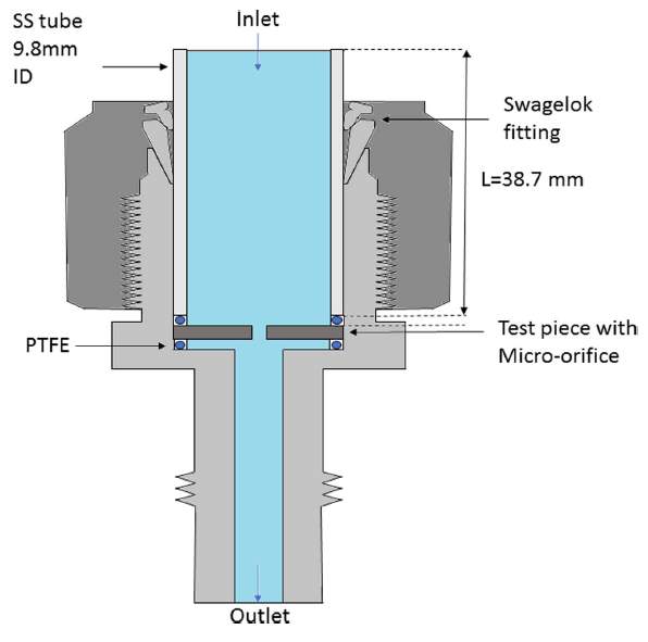
$C:\Users\Abdullah\Documents\SCHOOL\Mechanical Engineering Design - Master's\First Semester\60004 - Research Methods\test section 1.PNG$

Fig.1. Schematic of test section used in Cioncolini et al., (2017). Not to scale.

The test section was connected to a flow loop that could deliver micro-filtered and high purity water at the desirable variable conditions i.e. temperature, pressure and volumetric flow rate Cioncolini et al., (2017).

3. Methodology

In order to recreate the experiment done in the study above, simulations were carried using ANSYS FLUENT 19.0. These simulations were 2D axisymmetric; therefore the entire geometry did not have to be created and could be simplified. A mesh sensitivity study was carried out in order to choose the best mesh which optimized time and computational cost. Once the optimal mesh was established, simulations at Re=100,000 – 220,000 were carried out in steps of Re=40,000 and different turbulence models, namely; k-ε, k-ω, Spalart-Allmaras and k-kl-ω.

A. Geometry

Due to the pipe and orifice both being of a circular nature, this allowed for simpler simulations to be carried out with ANSYS FLUENT i.e. 2D and axisymmetric. The geometry considered for the analysis was two 50mm diameter pipes upstream and downstream of the orifice. The length of the pipes was 50 times the diameter (2.5m) making the entire system 5.001m long. This provided that the flow upstream of the orifice was of uniform flow. The orifice itself was 0.3mm in diameter and 1mm in length (Cioncolini et al. 2017).

In ANSYS, a 2D geometry was created which only contained the top half of the pipes and orifice; the bottom line represented the axis of symmetry. Therefore the inlet and outlet were 25mm in length and the orifice 0.15mm. Fig.2-4 below shows the geometry. The geometry was also split into five sections to aid with the meshing. Length of section 2 and 4 were made to be the same as the height, 25mm

Orifice (3)

Centreline (Axis of symmetry)

Fig.2. Schematic view of geometry (not to scale)

25mm

2475mm

1mm

25mm

0.3mm

Fig.3. Schematic view of geometry with dimensions (not to scale)

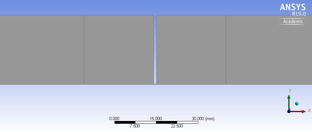
Fig.4. Geometry in ANSYS

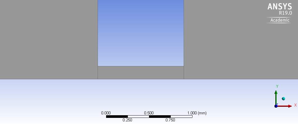
Fig.5. Orifice section of geometry (close up).

B. Mesh Sensitivity Study

In order to acquire the optimal mesh for the system without errors, a mesh sensitivity study was carried out first. This is done in order to minimize computation and simulation time and cost. A simulation is only as good as the quality of the mesh. The mesh generated for the geometry used two different kinds of elements, namely quadrilateral and triangular. The quadrilateral elements were used in sections 1, 3 and 5 whereas the triangular elements were used in sections 2 and 4.

Triangular elements used in sections 2 and 4 were used due to the sudden change in geometry. Its edges adjacent to the orifice were split into divisions using ‘’Edge Sizing’’ feature and biased with a bias factor of 1000. For the mesh sensitivity study, only the biased edges of sections 2 and 4 and the orifice edges were altered. Edges sections 1 and 5 of the inlet and outlet pipes were untouched as changing them had no significant effect on the final results. They were kept to having 400 divisions on the horizontal edges and 10 divisions on the vertical edges.

The number of divisions along the edges of the orifice and those adjacent to the orifice are summed up in Table.1 as well as the total number of elements in the mesh. During the study, the maximum velocity occurring in the system at an orifice Reynolds number of 100,000 while using the k-epsilon turbulence model was observed. Fig.10. shows the maximum velocity levelling off by the 7^th mesh density. Hence, the 7^th mesh was chosen as the optimal mesh and used for analysis.

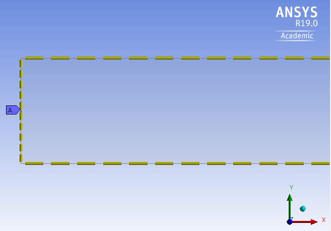
Fig.6. Edge divisions on inlet, outlet and pipe walls (Sections 1 and 5).

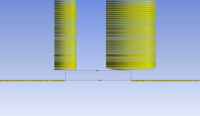
Fig.7. Biased edges leading to orifice.

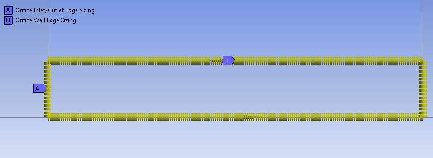
Fig.8. Orifice inlet, outlet and wall edge sizing.

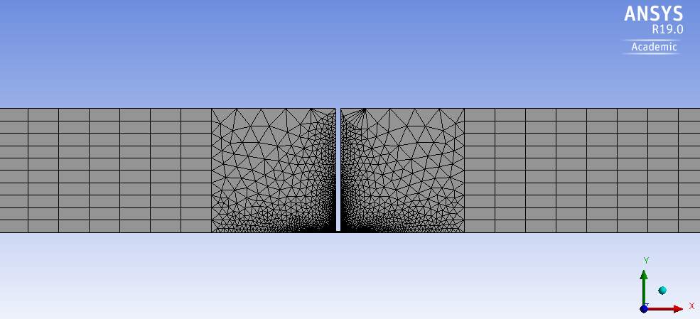
Fig.9. Mesh used for analysis.

Fig.10. Orifice mesh (close up). Table.1. Mesh Densities and Total Number of Elements

Mesh	Number of Divisions				Total Number of Elements
Mesh	Adj. orifice wall	Adj. orifice inlet/outlet	Orifice inlet/outlet	Orifice wall	Total Number of Elements
1	20	20	10	5	8960
2	40	40	20	10	10004
3	50	50	30	15	10900
4	70	70	40	20	12144
5	100	100	50	100	18156
6	150	150	80	160	28942
7	200	200	100	200	39236
8	220	220	120	240	49604
9	250	250	150	300	68092
10	270	270	170	340	82564

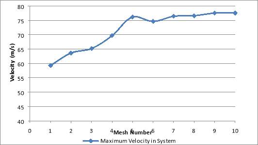
Fig.11. Maximum velocities observed after each simulation.

C. Setup and Boundary Conditions

Before the simulations could be run, boundary conditions had to be set in order to best replicate the experiment carried out in Cioncolini et al. (2017). The wall functions as well as the inlet and outlet had to be set. The simulations undergone in FLUENT were 2D, had double precision and run on serial processors. See Fig.12.

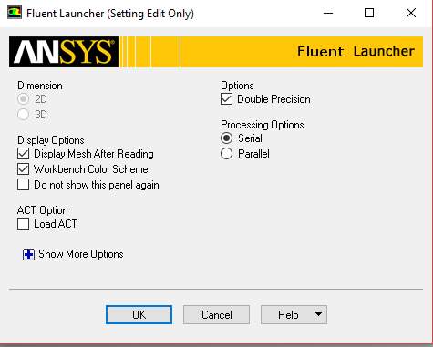
Fig.12. FLUENT Launcher

On starting FLUENT, on the ‘General’ setup task page, the type of solver to be used was selected; pressure or density based as well as the ‘Velocity Formulation’, ‘Time’, and ‘2D Space’. This is where the velocity formulation was set to absolute, the 2D space to be axisymmetric and the simulation to be a steady state simulation.

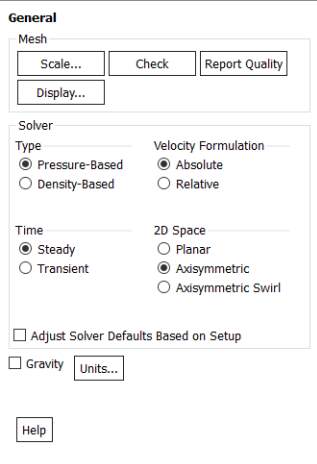
Fig.13. FLUENTGeneral task page

Experiments done in Cioncolini et al. (2017) had orifice Reynolds numbers ranging from 28,000 – 220,000. Using the Reynolds number and conservation of mass flow rate equations, Eq. (3) and (4) respectively, the average velocity at the inlet could be calculated. The Reynolds number is defined as: Re=ρVodμ (3) Where, Vo is the average velocity in the orifice, d is the orifice diameter and μ is the viscosity of water.

The conservation of mass flow rate is defined as: ṁ=ρAV=constant (4) ∴ ρAiVi=ρAoVo (5) Where Ai and Ao are the inlet and orifice cross sectional areas respectively and Vi is the average inlet velocity. From Eq. (3), a simplified equation for the average inlet velocity can be derived. Vi=dD2×Vo (6) Where D is the diameter of the inlet. The velocity obtained from Eq. (6) was used to set the inlet velocity.

The outlet was set to a pressure outlet with a gauge pressure of 0. The axis of symmetry (see Fig. 2) was set to centreline conditions. This meant that the remaining edges were set to have non-slip wall conditions. As mentioned in Cioncolini et al. (2017), the fluid, water, used for the experiments was at 503K and 12MPa. Using information from Peacesoftware.de (2018) the properties of water at said temperature and pressure was input into FLUENT and used for the simulations.

Before the simulations could be run, initialization had to take place which was done using the ‘’Hybrid Initialization’’ feature within FLUENT. The residuals were set to 1× 10^-6. The simulations were set to undergo 2000 iterations before stopping as this would be enough to achieve convergence. Fig. 14-17 shows the convergence history for the turbulence models used.

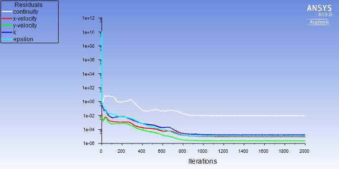
Fig.14. Convergence history of the k-ε model.

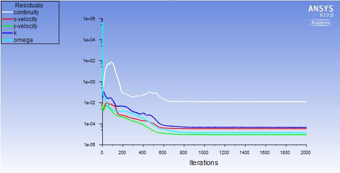
Fig.15. Convergence history of the k-ω model.

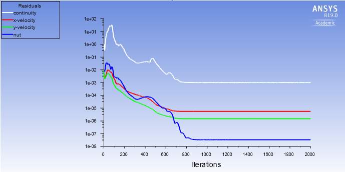
Fig.16. Convergence history of the Spalart-Allmaras model.

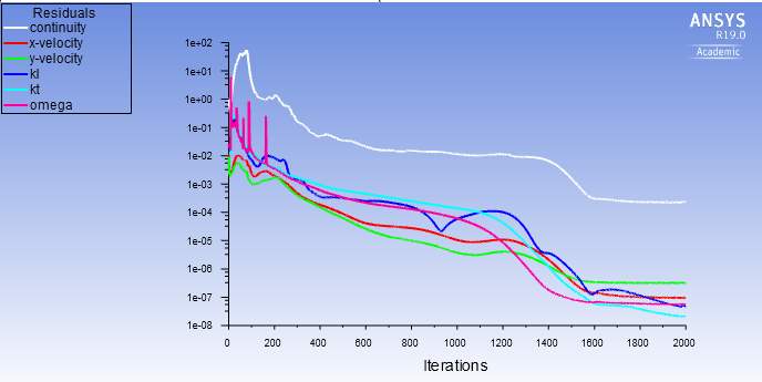
Fig.17. Convergence history of the k-kl-ω model

D. Governing Equations and Turbulence Models

While carrying out simulations with ANSYS FLUENT, the solver either uses the pressure based or density based solver. The pressure based solver is generally used for incompressible flows whereas the density based solver is used for compressible flows (Afs.enea.it, 2018). Since the flow through the orifice is assumed to be incompressible, the pressure based solver was used.

Regardless of the solver used, the software uses the Navier –Stokes equations to determine the behaviour of the fluid (Afs.enea.it, 2018). These equations include the conservation of mass and momentum shown in (7) and (8) respectively. ∇∙ρv⃗=0  (7) ∇∙ρv⃗vi=-δpδxi+∇∙μl+μt∇vi+Si (8) Where ρ is the density, v⃗ is the velocity vector, vi is the ith component of the velocity vector, μl and μt are the laminar and turbulent dynamic viscosities respectively and Si is the added source term (Edmunds et al., 2016).

Eq. (7) and (8) above, along with a turbulence model selected are solved by FLUENT to describe the behaviour of the fluid. The different turbulence models used during the analysis are explained in the literature.

i) k-ε Realizable Turbulence Model

This is a two equation turbulence model and is the most popular. Various types of k-ε turbulence models exist such as the Standard k-ε, k-ε RNG and Realizable k-ε. All of these models calculate the turbulent kinetic energy, k and the turbulent dissipation rate, ε. The difference between these models lies within the turbulent dissipation rate equation (Lateb et al., 2013). The realizable k-ε also contains a new equation for the turbulent viscosity.

The turbulent kinetic energy and dissipation rate are shown in Eq. (9) and (10) respectively according to a FLUENT User Guide, Sharcnet.ca (2018). ∂∂tρk+∂∂xjρkuj=∂∂xjμ+μtσk∂k∂xjGk+Gb-ρϵ-YM+Sk (9) ∂∂tρϵ+∂∂xjρϵuj=∂∂xjμ+μtσϵ∂ϵ∂xj+ρC1Sϵ-ρC2ϵ2k+vϵ+C1ϵϵkC3ϵGb+Sϵ (10) Where C1=max0.43,ηη+5, η=Skϵ, S=2SijSij Gk is the generation of turbulence kinetic energy due to the mean velocity gradients, Gb is the generation of turbulence kinetic energy due to buoyancy, YM is the contribution of the fluctuating dilatation in compressible turbulence to the overall dissipation rate, C1 and C2 are constants, σk and σϵ are turbulent Prandtl numbers for k and ε respectively and Sk and Sϵ are source terms (Sharcnet.ca, 2018).

ii) Standard k-ω Turbulence Model

Similar to the k-ε model, the k-ω turbulence model is also a two equation model. This model calculates the turbulent kinetic energy as well however instead of dissipation rate, ε, it calculates another parameter known as the dissipation per unit turbulence kinetic energy, ω i.e. ratio of ε to k (Wilcox, 1998). The equations for k and ω used in ANSYS FLUENT are shown in Eq. (11) and (12) respectively.

∂∂tρk+∂∂xiρkui=∂∂xjΓk∂k∂xj+Gk-Yk+Sk (11) ∂∂tρω+∂∂xiρωui=∂∂xjΓω∂ω∂xj+Gω-Yω+Sω (12) Where Gb is the generation of ω, Γk and Γω are the effective diffusivity of k and ω respectively, Yk and Yω are the dissipation of k and ω due to turbulence and Sk and Sω are source terms (Sharcnet.ca, 2018).

iii) Spalart - Allmaras Turbulence Model

Unlike the k-ε and k-ω models, the Spalart-Allmaras model is a simple one equation turbulence model that solves a transport equation for a turbulent viscosity, ν (Pellerin, Leclaire and Reggio, (2015), Nordanger et al. (2015), Shukla and Kaviti, (2017)). As stated in Wilcox (1998), one equation models are incomplete because they relate the turbulence length scale to a typical flow dimension, whereas two equation models are complete because they can predict the characteristics of a turbulent flow without previously knowing the turbulence structure and provide an equation for the turbulence length scale. The transport equation for the Spalart – Allmaras model in FLUENT is shown in Eq. (13). The variable is ν.

∂∂tρν̃+∂∂xiρν̃ui=Gv+1σṽ∂∂xjμ+ρν̃∂ν̃∂xj+Cb2ρ∂ν̃∂xj2-Yν+Sν̃ (13) Where Gv is the production of turbulent viscosity, Yν is the destruction of turbulent viscosity in the near wall region, Cb2 and σṽ are constants, v is the molecular kinematic viscosity and Sν̃ is a source term (Sharcnet.ca, 2018). iv) k-kl-ω Transition Turbulence Model The k-kl-ω transition is a three equation turbulence model that is usually used for incompressible low Reynolds number flows to predict the development of the boundary layer and the transition of the flow from the laminar to the turbulent regime (Sharcnet.ca, 2018, Openfoam.com, 2018).

The transport equations for this turbulence model are the turbulent kinetic energy (k_T), laminar kinetic energy (k_L) and inverse turbulent time scale (ω) (Sharcnet.ca, 2018) shown in Eq. (14), (15) and (16) respectively. DkTDt=PKT+R+RNAT-ωkT-DT+∂∂xjν+αTαk∂kT∂xj (14) DkLDt=PKL-R-RNAT-DL+∂∂xjν∂kL∂xj (15) DωDt=Cω1ωkTPKT+CωRfw-1ωkTR+RNAT-Cω2ω2+Cω3fωαTfW2kTd3+∂∂xjν+αTαω∂ω∂xj (16)

The constants used in this model are available in Sharcnet.ca (2018) and are already inbuilt into FLUENT. Further descriptions of the constants can also be found in Walters and Cokljat (2008).

4. Results

In order to calculate the dimensionless pressure drop across the orifice, 1000 data points were taken at distances equivalent to one diameter length of the pipe upstream and downstream of the centreline of the orifice. These data points were used to plot the dimensionless pressure drop against the Reynolds number as well as the square root of the pressure drop against the volumetric flow rate. The pressure drops recorded across the orifice were used in Eq. (1) and used to plot Fig. 34, along with Eq. (2).

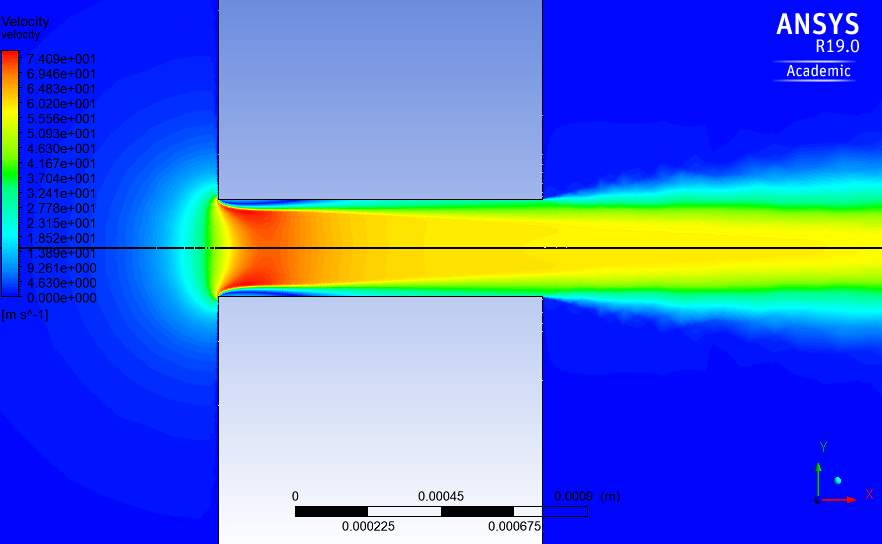
Fig.18. Velocity contour through orifice with k-ε turbulence model at Re=100,000.

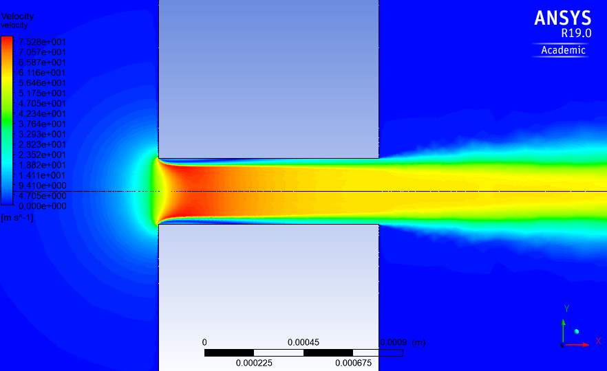
Fig.19. Velocity contour through orifice with k-ω turbulence model at Re=100,000.

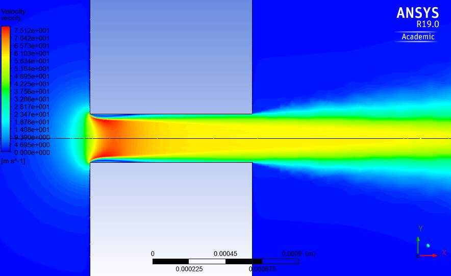
Fig.20. Velocity contour through orifice with Spalart-Allmaras turbulence model at Re=100,000.

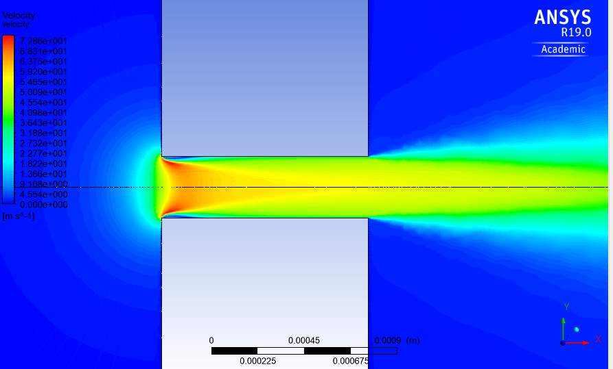
Fig.21. Velocity contour through orifice with k-kl-ω turbulence model at Re=100,000.

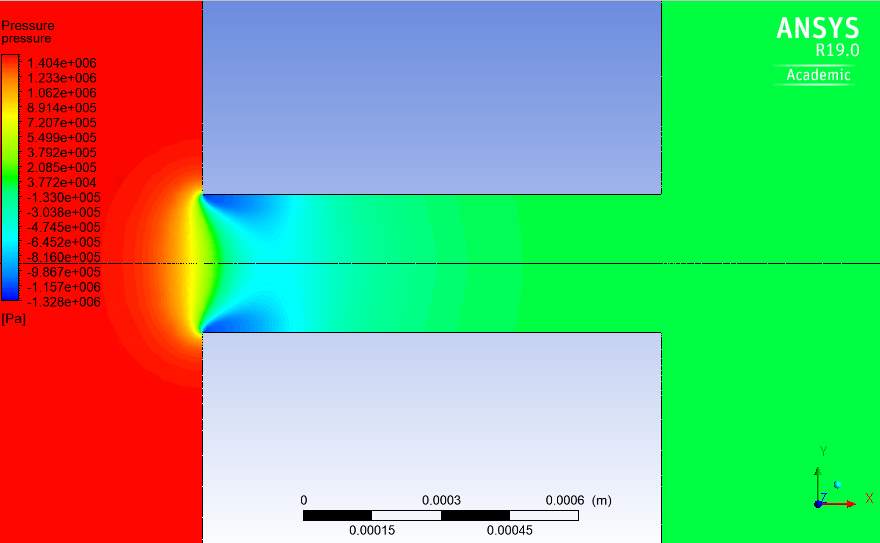
Fig.22. Pressure contour through orifice with k-ε turbulence model at Re=100,000.

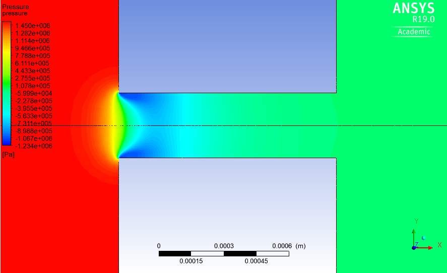
Fig.23. Pressure contour through orifice with k-ω turbulence model at Re=100,000.

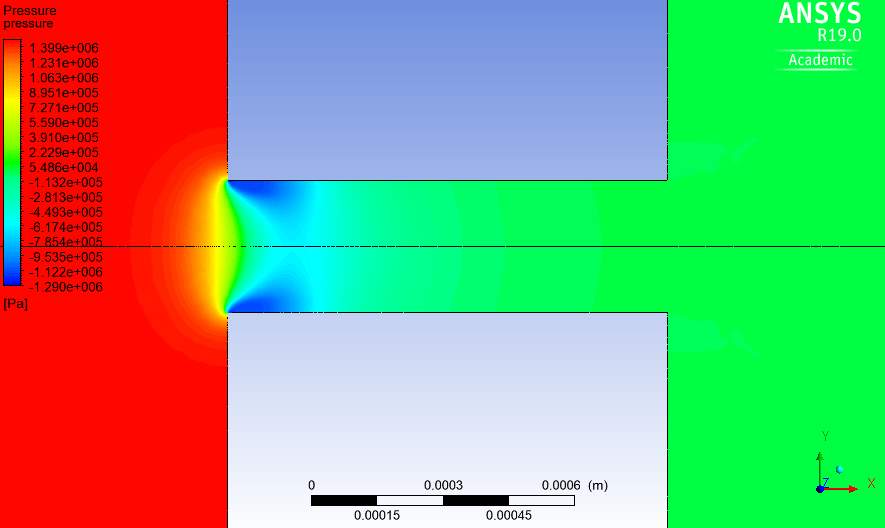
Fig.24. Pressure contour through orifice with Spalart-Allmaras turbulence model at Re=100,000.

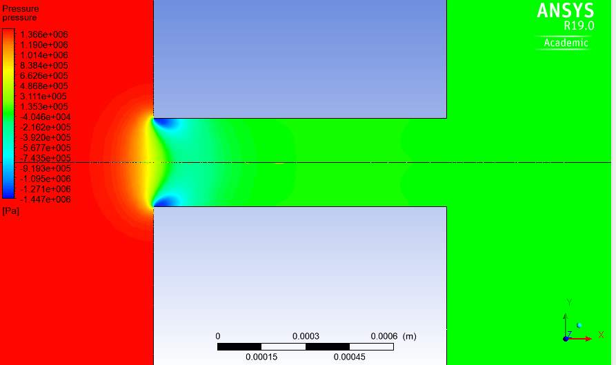
Fig.25. Pressure contour through orifice with k-kl-ω turbulence model at Re=100,000.

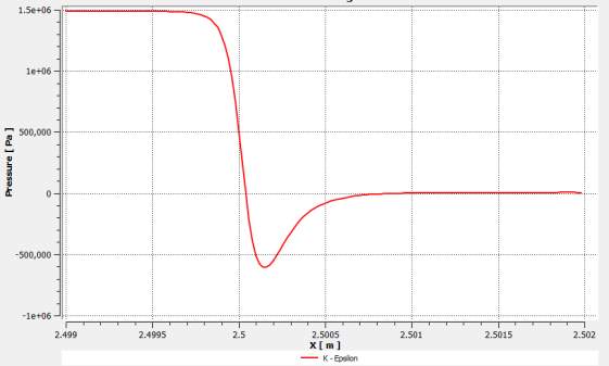
Fig.26. Pressure drop within the orifice for the k-ε model at Re=100,000.

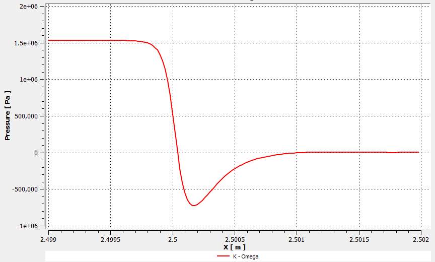
Fig.27. Pressure drop within the orifice for the k-ω model at Re=100,000.

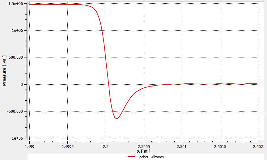
Fig.28. Pressure drop within the orifice for the Spalart-Allmaras model at Re=100,000.

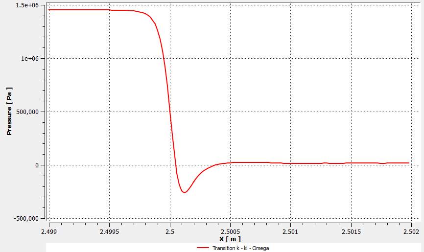
Fig.29. Pressure drop within the orifice for the k-kl-ω model at Re=100,000.

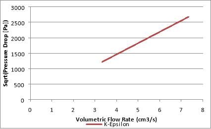
Fig.30. Square root of pressure drop across orifice in relation to volumetric flow rate with k-ε turbulence model

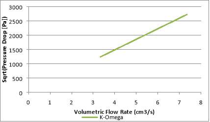
Fig.31. Square root of pressure drop across orifice in relation to volumetric flow rate with k-ω turbulence model

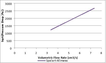
Fig.32. Square root of pressure drop across orifice in relation to volumetric flow rate with Spalart-Allmarasturbulence model

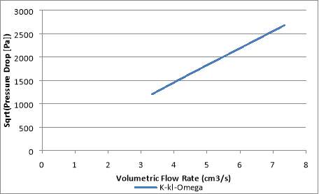
Fig.33. Square root of pressure drop across orifice in relation to volumetric flow rate with k-kl-ω turbulence model

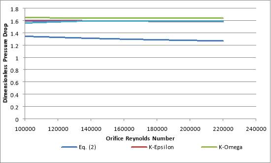
Fig.34. Comparison between the different turbulence models used and Eq. (2). Note that the k-ε series is being overlapped by the Spalart-Allmaras series. Table.2. Pressure Drops Observed.

Reynolds Number	Pressure Drop (kPa)
Reynolds Number	*k-ε*	*k-ω*	Spalart-Allmaras	*k-kl-ω*
100,000	1489	1534	1483	1454
140,000	2914	3000	2903	2909
180,000	4805	4950	479.3	4800
220,000	7171	7385	7143	7177

Table.3. Dimensionless Pressure Drop.

Reynolds Number	Dimensionless Pressure Drop, K
Reynolds Number	*k-ε*	*k-ω*	Spalart-Allmaras	*k-kl-ω*	Eq. (2)
100,000	1.598	1.646	1.592	1.560	1.343
140,000	1.596	1.642	1.589	1.593	1.310
180,000	1.591	1.639	1.587	1.590	1.286
220,000	1.590	1.637	1.584	1.591	1.267

5. Discussion

A. Velocity Contours

The velocity contours for the flow through the orifice with the different turbulence models used at Re=100,000 is shown in Fig.18-21. The profiles are similar at different Reynolds numbers except for the magnitude of velocity. These profiles show the flow upstream of the orifice having a near 0 velocity magnitude. This is expected, as according to Eq. (6) in order to achieve the desired Reynolds number in the orifice, the inlet velocity would have to be very small.

For example, to produce an orifice Reynolds number of 100,000, the inlet velocity would have to be set to 0.0017m/s. The contours show the velocity increase rapidly as the water approaches the orifice. This is expected of the flow as the mass flow rate is conserved and the water follows the principle of the venture effect, which refers to the fluid increasing in velocity as the cross sectional area is decreased (Blocken et al., 2011).

The water reaches maximum velocity shortly after entering the orifice, around 75m/s and then reducing to around 55m/s for the remainder of the orifice. At where the velocity is maximum in the orifice, a boundary layer is seen to have begun forming on the orifice walls with the k-ω model predicting a longer and thicker boundary layer. This turbulence model also predicts a greater area of maximum velocity occurring.

A jet is seen to form once the water exits the orifice. The velocity of this jet gradually decreases on the outside moving inwards. The transition turbulence model i.e. k-kl-ω shows a very small area in the orifice where the velocity reaches its maximum which translates into the model predicting the lowest maximum velocity in the orifice. The boundary layer predicted in this model as well is the smallest compared with the other models. I contrast to the boundary layer and maximum velocity, the three-equation model predicts the largest jet downstream of the orifice.

B. Pressure Contours

The pressure contours of Fig.22-25 are also predicted as expected. This includes a high pressure gradient upstream of the orifice and the pressure reducing while the velocity increases on approaching the orifice. This is typical of single-phase flow of liquids.

The pressure is also seen to stabilize as the velocity does as well. Similar to the velocity contour, the k-ω pressure contour predicts a greater area of low pressure in the orifice compared to the other models while the k-kl-ω model predicts the smallest. The behaviour and change in the pressure at a Reynolds number of 100,000 is shown in Fig. 26-29.

They show how the pressure changes at 1mm before and after the orifice on the centreline or axis of symmetry. Therefore, starting from the inlet, the measurements were taken from 2.499 – 2.502m. The orifice lies between 2.5 – 2.501m. Similar to the pressure contours above, the pressure is relatively stable upstream of the orifice.

The pressure decreases rapidly just before entering the orifice and continues decreasing inside the orifice until the water reaches maximum velocity and then increases again. Within the orifice the pressure becomes stable again at almost 0Pa just like the respective contour plots.

C. Volumetric Flow rate and Pressure

Fig.30-33 show the square root of the pressure drop (Pa) plotted against the volumetric flow rate of the water in the orifice (cm³/s). These figures show a linear relationship between the square root of the pressured drop and volumetric flow rate. This means that the relationship between the pressure drop and the volumetric flow rate is quadratic and is expected of single-phase flow. This was stated earlier in the literature and also seen in Cioncolini et al. (2017).

D. Dimensionless Pressure Drop

Fig.34 shows the dimensionless pressure drops of Eq. (2) and the different turbulence models, calculated from Eq. (1), plotted against the orifice Reynolds number ranging from 100,000 – 220,000. As seen in Cioncolini et al. (2017), the dimensionless pressure drop slightly decreases as the Reynolds number increases.

This study shows the dimensionless pressure drop almost remaining constant with increasing Reynolds number for the different turbulence models however at the same time, the dimensionless pressure drops predicted are higher than that of Eq.(2). The difference in the dimensionless pressure drop between the simulation and Eq. (2) are in the range of 18-29% with the k-ω model with the highest percentage difference.

Although the simulations do predict the dimensionless pressure drop to decrease very slightly for the k-ε, k-ω and Spalart-Allmaras models, as seen in Table 3 the decrement is not at the same rate as Eq. (2) and can be stated to be negligible. Eq. (2) produces a steeper negative gradient. The k-kl-ω however is seen to very slightly increase and decrease. These changes are very small and can also be said to be negligible. The k-kl-ω model is in very close relation with the k-ε model and Spalart-Allmarasmodel, hence covering the k-ε and Spalart-Allmaras series in Fig.34.

Ultimately the simulations predict a constant dimensionless drop whereas in the experiment the dimensionless pressure drop decreases slightly as the Reynolds number increases. Therefore none of the turbulence models used in this study accurately recreates the experimental results from Cioncolini et al. (2017).

6. Conclusion

Following the experiments done in Cioncolini et al., (2017), computational fluid dynamics was used to recreate the experiments and simulate the flow through the orifice using ANSYS FLUENT 19.0. The simulations done were consisted of a 2D axisymmetric geometry which simplified the simulations to be carried out. The fluid used was water at 12MPa and 503K. The properties of water at these conditions was acquired from Peacesoftware.de (2018) and input into FLUENT.

Before the main simulations could run, a mesh sensitivity study was carried out to find out which mesh would provide the most adequate results while optimising time and computational cost. The mesh sensitivity study consisted of ten different meshes with different densities, increasing in number of elements from 1-10. Once the optimum mesh was selected, simulations were carried out using four different turbulence models namely, k-ε realizable, standard k-ω, Spalart-Allmaras and k-kl-ω transition turbulence models.

The simulations for each turbulence model had orifice Reynolds numbers ranging from 100,000 – 220,000 in steps of Re=40,000. The results from these simulations were used to compute the dimensionless pressure drop (K) across the orifice using Eq. (1). Unlike in Cioncolini et al., (2017) where the dimensionless pressure drop slightly decreased with increasing Reynolds number, here, the change in dimensionless pressure drop, K, was negligible and predicted to be constant.

The contour plots and results obtained showed the pressure to drastically decrease upon entrance into the orifice and reach minimum within before increasing to near 0 before exiting. The velocity on the other hand increased and reached maximum where the pressure reaches its minimum in the orifice. It then levels off around 50-60m/s.

The volumetric flow rate and pressure drop (Pa) show a quadratic relationship between the two. In conclusion the results from the simulations were in disagreement with the experimental results as they did not predict the dimensionless pressure drop to slightly decrease with increasing Reynolds number, instead it predicted the dimensionless pressure drop to be constant.

Future work is recommended to be carried out on the turbulence models used or whether better results will be obtained in using a 3D simulation such as Large Eddy Simulation (LES) or Direct Numerical Simulation (DNS).

7. References

Afs.enea.it. (2018). ANSYS FLUENT 12.0 Theory Guide - 18.1 Overview of Flow Solvers. [online] Available at: http://www.afs.enea.it/project/neptunius/docs/fluent/html/th/node360.htm [Accessed 11 Aug. 2018].

Beinert, S.; Gothsch, T.; Kwade, A. Numerical evaluation of stresses acting on particles in high-pressure microsystems using a Reynolds stress model. Chem. Eng. Sci. 2015, 123, 197–206.

Blocken, B., van Hooff, T., Aanen, L. and Bronsema, B. (2011). Computational analysis of the performance of a venturi-shaped roof for natural ventilation: Venturi-effect versus wind-blocking effect. Computers & Fluids, 48(1), pp.202-213.

Cfd-online.com. (2017). K-epsilon models -- CFD-Wiki, the free CFD reference. [Online] Available at: https://www.cfd-online.com/Wiki/K-epsilon_models [Accessed 7 Dec. 2017].

Chisholm, D. (1983). Two-phase flow in pipelines and heat exchangers. London [usw.]: Godwin Cioncolini, A., Cassineri, S., Duff, J., Curioni, M. and Scenini, F. (2017). Micro-orifice single-phase flow at very high Reynolds number. Experimental Thermal and Fluid Science, 91, pp.35-40.

Cioncolini, A., Scenini, F. and Duff, J. (2015). Micro-orifice single-phase liquid flow: Pressure drop measurements and prediction. Experimental Thermal and Fluid Science, 65, pp.33-40.

Comsol.com. (2017). What Are the Navier-Stokes Equations? [online] Available at: https://www.comsol.com/multiphysics/navier-stokes-equations [Accessed 4 Dec. 2017].

Durst, F. and Wang, A. (1989). Experimental and numerical investigations of the axisymmetric, turbulent pipe flow over a wall-mounted thin obstacle. In: 7th Symposium on Turbulent Shear Flows.

Edmunds, M., Williams, A., Masters, I. and Croft, T. (2016). An enhanced disk averaged CFD model for the simulation of horizontal axis tidal turbines. Renewable Energy, 101, pp.67-81.

Eiamsa-ard, S., Ridluan, A., Somravysin, P. and Promvonge, P. (2008). Numerical investigation of turbulent flow through a circular orifice. KMITL Sci. J., 8(1), pp.43-50.

Far, E., Geier, M., Kutscher, K. and Krafczyk, M. (2017). Implicit Large Eddy Simulation of Flow in a Micro-Orifice with the Cumulant Lattice Boltzmann Method. Computation, 5(2), p.23.

Gothsch, T., Schilcher, C., Richter, C., Beinert, S., Dietzel, A., Büttgenbach, S. and Kwade, A. (2014). High-pressure microfluidic systems (HPMS): flow and cavitation measurements in supported silicon microsystems. Microfluidics and Nanofluidics, 18(1), pp.121-130.

Henderson, N., Pacheco, F. and Kischinhevsky, M. (2017). Numerical solution of the Navier-Stokes equations using the Path Tubes method. Chemical Engineering Science, 172, pp.585-602.

Jin, S., Sung, T., Kim, J. and Seo, T. (2011). Optimal design of a micro-orifice for constant evaporator superheat in a small cooler. Applied Thermal Engineering, 31(14-15), pp.2631-2635.

Kojasoy, G., Landis, F., Kwame-Mensah, P. and Chang, C. (1997). Two-phase pressure drop in multiple thick- and thin-orifice plates. Experimental Thermal and Fluid Science, 15(4), pp.347-358.

Lateb, M., Masson, C., Stathopoulos, T. and Bédard, C. (2013). Comparison of various types of k–ε models for pollutant emissions around a two-building configuration. Journal of Wind Engineering and Industrial Aerodynamics, 115, pp.9-21.

Morrison, G., Deotte, R., Nail, G. and Panak, D. (1993). Mean velocity and turbulence fields inside aβ=0.50 orifice flowmeter. AIChE Journal, 39(5), pp.745-756

Nail, G. (1991). A study of 3-Dimensional flow through orifice meters. Ph.D. Texas A&M University. Nilpueng, K. and Wongwises, S. (2009). Experimental investigation of two-phase flow characteristics of HFC-134a through short-tube orifices. International Journal of Refrigeration, 32(5), pp.854-864.

Nordanger, K., Holdahl, R., Kvamsdal, T., Kvarving, A. and Rasheed, A. (2015). Simulation of airflow past a 2D NACA0015 airfoil using an isogeometric incompressible Navier–Stokes solver with the Spalart–Allmaras turbulence model. Computer Methods in Applied Mechanics and Engineering, 290, pp.183-208.

Oliveira, N., Vieira, L. and Damasceno, J. (2010). Numerical Methodology for Orifice Meter Calibration. Materials Science Forum, 660-661, pp.531-536

Peacesoftware.de. (2018). [online] Available at: http://www.peacesoftware.de/einigewerte/calc_dampf.php7 [Accessed 13 Aug. 2018].

Pellerin, N., Leclaire, S. and Reggio, M. (2015). An implementation of the Spalart–Allmaras turbulence model in a multi-domain lattice Boltzmann method for solving turbulent airfoil flows. Computers & Mathematics with Applications, 70(12), pp.3001-3018.

Shah, M., Joshi, J., Kalsi, A., Prasad, C. and Shukla, D. (2012). Analysis of flow through an orifice meter: CFD simulation. Chemical Engineering Science, 71, pp.300-309.

Sharcnet.ca. (2018). 4.5.1. Overview. [online] Available at: https://www.sharcnet.ca/Software/Ansys/16.2.3/en-us/help/flu_th/x1-1540005.16.1.html [Accessed 24 Aug. 2018].

Sharcnet.ca. (2018). 4.5.2. Transport Equations for the k-kl-ω Model. [online] Available at: https://www.sharcnet.ca/Software/Ansys/16.2.3/en-us/help/flu_th/flu_th_sec_turb_kkl_trans_eq.html [Accessed 24 Aug. 2018].

Sharcnet.ca. (2018). FLUENT 6.3 User's Guide - 12.4.3 Realizable - Model. [online] Available at: https://www.sharcnet.ca/Software/Fluent6/html/ug/node480.htm [Accessed 11 Aug. 2018].

Shukla, V. and Kaviti, A. (2017). Performance evaluation of profile modifications on straight-bladed vertical axis wind turbine by energy and Spalart Allmaras models. Energy, 126, pp.766-795.

Tu, X., Hrnjak, P. and Bullard, C. (2006). Refrigerant 134a liquid flow through micro-scale short tube orifices with/without phase change. Experimental Thermal and Fluid Science, 30(3), pp.253-262.

Ushida, A., Hasegawa, T., Narumi, T. and Nakajima, T. (2013). Flow properties of nanobubble mixtures passing through micro-orifices. International Journal of Heat and Fluid Flow, 40, pp.106-115.

Walters, D. and Cokljat, D. (2008). A Three-Equation Eddy-Viscosity Model for Reynolds-Averaged Navier–Stokes Simulations of Transitional Flow. Journal of Fluids Engineering, 130(12), p.121401.

Wilcox, D. (1998). Turbulence modeling for CFD. La Cañada, Calif: DCW Industries. X. Wang, Q. Lin, Y. Tai, A parylene micro check valve, in: 12th IEEE International Conference on Micro Electro Mechanical Systems, Orlando-FL, USA, 1999.