Shape memory polymer are advanced class of active polymers that have dual shape capability where they change shape in a predefined way. They are materials with properties that change in response to external factors. The external factor is temperature and the property to be young’s modulus. Polylactic Acid is a good example of shape memory polymer. Polylactic Acid (PLA) is a biodegradable polymer with a lot of applications in tissue regeneration and repair.

Although the basic concept of shape memory polymer has been known, recent progresses have challenged the accepted understanding of the polymer shape memory effects. In this dissertation, the effect of temperature on shape memory polymer was investigated. A differential scanning calorimetry (DSC) has been used to analyse the effect of temperature on shape memory. the thermolytic technique was used to investigate the amount of heat required and how it affected the shape memory polymer in elasticity, crystallisation and shrinkage force.

Polylactic Acid (PLA) samples were expanded at various temperatures between 50^oc and 65^oc and a rate between 50mm/min and 100mm/min. Polylactic Acid (PLA) samples were crystallised at various temperatures between 65^oc and 100^oc and a rate between 50mm/min and 100mm/min. Polylactic Acid (PLA) samples were shrunk at various temperatures between 55^oc and 60^oc and a rate between 50mm/min and 100mm/min. it is seen that temperature has effects on Polylactic specimens. It is seen that the increase in temperature gives increase to expansion and crystallinity while increase in temperature leads to decrease in shrinkage force.

The main conclusion to draw from this study, the results suggest that temperature influences Polylactic Acid (PLA) and further long term studies must be conducted to explore this fully.

Keywords: Shape memory polymer, Elasticity, Crystallisation, Shrinkage force.

INTRODUCTION

There has been significant attention on the functionality and usefulness of shape memory polymer. Shape-Memory Polymers are a rising class of polymers, that can be applied in various areas of life (Behl and Lendlein, 2007). Shape Memory Polymer can be defined as a polymer which can be distorted and afterwards fixed which stays stable for a brief period unless it is exposed to suitable external factors that initiate the polymer to recover to its original shape (Xie, 2011). There are different forms of external factors that may be employed as the recovery trigger but the most common one is heating that leads to a temperature increase. Behl and Lendlein (2007) states that “Shape memory polymer can change their shape in a predefined way from Shape A to B when exposed to a suitable factor”. Shape memory Polymers applications include self – deployable sun sails in spacecraft, heat – shrinking tubes for electronics or films for packaging, intelligent medical devices.

The behaviour related to Shape Memory Polymer is known as polymer shape memory effect (Xie, 2011). Xie (2011) states that, “The first recognition of polymer Shape Memory Effect can be traced back to a patent in 1940s. The well-known heat shrinkage tubing that appeared in 1960 shows the commercial application of Shape Memory Polymer. It is thought that the first official use of Shape Memory Polymer may have started in have started in 1984, with the development of the polynorbornene based SMP by CDF Chimie Company (France). Despite the long history of SMP, however, the phenomenon of polymer SME had remained little known and the scientific paper in this area had been rather limited until 1990s”.

Polymer can be defined as any numerous natural and synthetic compounds of usually high molecular weight consisting of up to millions of repeated linked units, each relatively light and simple molecule (TheFreeDictionary.com, 2017). Polymers are made the transformation of small molecules known to be called MONOMER. (Faculty.uscupstate.edu, 2017) states that “Although the chemical properties of polymers are similar to those of analogous small molecules, their physical properties are quite different”. Polymer due to the its variation in properties and, can be used wide range of applications and industries by controlling the how the polymer is being processed. Polylactic Acid (PLA) is said to be one of the most important bio-materials due to its biocompatibility (compatibility with living tissues or a living system by not being toxic, injurious, or physiologically reactive and not causing immunological rejection), good mechanical properties and degradation rate.

BIOMATERIALS

Biomaterials according to (Merriam-webster.com, 2017), a natural or synthetic materials that is suitable for introduction into living tissue especially as part of a medical (as an artificial joint). Polymeric Biomaterials are one of the cornerstones of tissue engineering. The main factor for polymeric biomaterials is that it must be biocompatible. (Ulery, Nair and Laurencin, 2017) states that “In order to meet the needs of the biomedical community, materials composed of everything from metals and ceramics to glasses and polymers have been researched. Polymers possess significant potential since flexibility in chemistry gives rise to materials with great physical and mechanical property diversity. Degradable polymers are of utmost interest since these biomaterials are able to be broken down and excreted or resorbed without removal or surgical revision.” There are varieties of biomaterial which has been researched upon and used clinically. Biomaterial Polymers are widely used and they are manufactured to adapt to their use. (Sciencing, 2017) states the advantages of biomaterials – “The main advantage of biomaterial polymer is that they are all biodegradable and due to the interaction with the body, they absorb important nutrients and water from the blood.”

POLYMER MORPHOLOGY

Morphology can be defined as the study of shape. (Unterlasslab.com, 2017) defined morphology as the study of the microscopic appearance of a polymeric material. According to (Faculty.uscupstate.edu, 2017), “Polymer Morphology is the overall form of polymer structure, including crystallinity, branching, molecular weight, cross-linking etc.”.

Small molecules contain crystalline solids, which are highly-ordered 3 – dimensional arrays of molecules. Solid polymers can be crystalline or amorphous ([Encyclopedia Britannica, 2017], defined Amorphous solid, as any noncrystalline solid in which the atoms and molecules are not organised in a definite lattice pattern). Highly crystalline polymers are rigid, high melting and less affected by solvent penetration. Crystallinity makes a polymer strong, but also lowers their impact resistance (Faculty.uscupstate.edu, 2017).

The morphology of the crystals and the degree of crystallinity depends on the type and structure of the polymer and on the growth conditions. Narrow molecular weight, linear polymer chains and high molecular weight increase the crystallinity. Chain disorder or misalignment, which is common, leads to amorphous material since twisting, kinking and coiling prevents strict ordering required in the crystalline state. (Virginia.edu, 2017) states that “linear polymers with small side groups, which are not too long form crystalline regions easier than branched, network, atactic polymers, random copolymers, or polymers with bulky side groups”. Crystalline polymers are denser than amorphous polymers, so the degree of crystallinity can be obtained from the measurement of density.

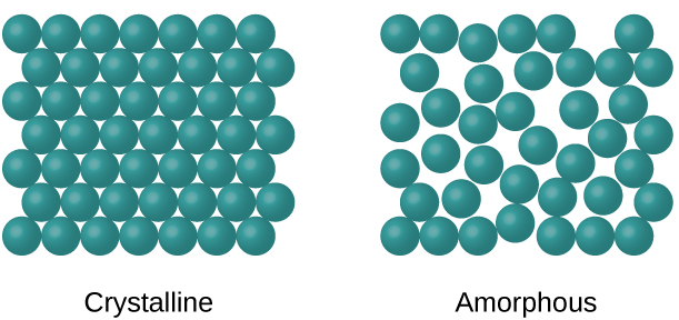
Figure 1: Diagram Showing Polymer Morphology.

CRYSTALLISATION KINETICS

(Long, Shanks and Stachurski, 1995) defined Crystallisation as the process of phase transformation. (Hobbs, 2004), states that crystallization kinetics is the area of polymer science that deals with the rate at which randomly ordered chains transform into highly ordered crystals, and include every aspect of the resultant structure that is dependent on the route that was taken between those different states.

(Jenkins, 1972), states the development of crystallinity in polymer involves two stages: NUCLEATION and GROWTH. Growth can take place from the pure molten polymer when it is cooled to below its melting point. There is no essential difference between the two processes, as a polymer diluted by a solvent has a melting point and crystallisation range, in just the same way as the pure polymer. According to (Jenkins, 1972), growth occurs between the melting point, Tm (of the pure polymer or of a solution), because the crystalline state is thermodynamically more stable. As the crystallisation temperature, Tc, is decreased (which is: as the degree of super cooling, ΔT = Tm – Tc, is increased), the rate increases.

The Nucleation is the step which determines whether or not the growth of crystalline units is to take place. Nucleation can occur in two ways, it can either be a homogenous process or a heterogeneous process. According to (“Homogenous Nucleation”), a nucleation with preferential nucleation sites is known as Homogenous Nucleation. Homogenous Nucleation occurs spontaneously and randomly but it requires either superheating or super cooling of the medium. It occurs with much more difficulty in the interior of a uniform substance. The creation of a nucleus implies the formation of an interface at the boundaries of a new phase. Heterogenous Nucleation involves the assumption that sites are present which are different in some way from the bulk composition of the polymer. They may be chemically modified points on the polymer chains, catalyst debris or other forms of impurity but main essential feature must be, that they enable polymer chains to be ordered on their surface, more easily than for homogenous nucleation.

(Sharples, 1966) states that, Homogeneous nucleation involves the spontaneous aggregation of polymer chains below the melting point, in a manner which is reversible up to the point where a critical size is reached. The theoretical treatment of homogenous, sporadic nucleation is based on the ideas developed by Turnbull and Fisher, and the results in a relation between nucleation rate, N, and Temperature, of the following form;

N= N0exp⁡(-ED/KT- ΔG*/KT

From the equation above, ED is the activation energy for the transport across the surface of the nucleus, ΔG* is the free-energy of formation of the critical size nucleus. For a three-dimensional nucleus, ΔG* is proportional to

Tm2/ΔT2

, where Tm is the melting point and ΔT is the degree of super-cooling. At small degrees of super-cooling, the nucleation rate will increase very rapidly with decreasing temperature of crystallisation.

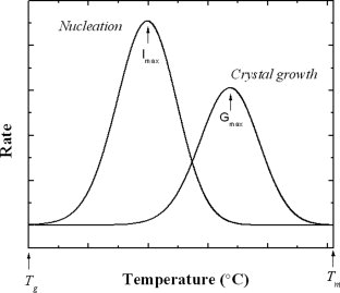
Figure 2: Diagram Showing the Graph of Nucleation and Growth

At much lower temperatures, the

-ED/KT

term dominates, so that Nucleation Rate (N), passes through a maximum, and subsequently decreases with temperature, until the glass point is reached.

Heterogenous Nucleation according to (Ronca, 2017), involves the aggregation of polymer chains at the interface with a foreign phase which could either be an adventitious impurity or a purposely added nucleating agent. The addition of nucleating agents increases the rate of nucleation and leads to the formation of a larger number and therefore smaller spherulites. Heterogenous nucleation requires a small degree of super-cooling, usually 10oc to 30oc which suggest that the most crystallisation of macromolecules is initiated during heterogenous nucleation.

Growth according to (Zhigilei, 2017), is the next step after nucleation. (Rosen, 1971) states that “not only are polymer chains often arranged to form crystallites, but these crystallites are often arranged in larger aggregates known as Spherulites”. These Spherulites grow radically from a point of nucleation until other spherulites are encountered. The size of the individual spherulites can be controlled by the number of nuclei present, more nuclei resulting in more but smaller spherulites. According to (Long, A. shanks and Stachurski, 1995), most polymers of sufficiently high crystallinity will show a spherulitic microstructure. Figure shows two basic types of spherulitic morphologies. Type I has a central nucleus from which crystalline lamellae initiate, growing radically, in all directions. The different crystal lamellae are nucleated separately and independently of each other. The spherical symmetry extends right to the centre of this type of spherulite. Type II spherulites essentially develop from one single lamella crystal; by continuous branching and fanning out, until a spherical shape is obtained but initially, in the centre, there is a unidirectional growth (parallel lamellae), which goes through a so-called sheaf stage.

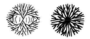
Figure 3: Diagram showing two forms of Spherulite

SHAPE MEMORY POLYMER

According to (Crgrp.com, 2017), Shape memory polymers are polymers whose qualities have been altered to give them dynamic shape memory properties. Using thermal or stimuli, Shape memory can exhibit a radical change from a rigid polymer to a very elastic state, then back to a rigid state. (Crgrp.com, 2017) stated that in its elastic state, it will recover its memory shape if left unrestrained.

(Whitwam, 2017) states this material can be stretched and contorted into almost any shape and then heat is applied. According to (Whitwam, 2017), the material has a definite shape, which it remembers despite twisting and stretching.

POLYLACTIC ACID

(Majid, Revati and Normahira, 2017), states “Poly(lactic) Acid (PLA) as a high versatile, biodegradable, aliphatic polyester derived from a renewable resource”. PLA (Polylactic Acid) belongs to the family of aliphatic polyesters commonly made from α – hydroxy acids (Averous, 2008). It has gotten a lot of attention in biomedical fields such as bones fixation material, drug carrier and tissue engineering since lactic is a chiral molecule (According to [Chemeddl.org, 2017], A molecule is not chiral if it is not superimposable on its mirror image).

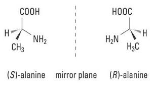
Figure 4: Diagram Showing a Chiral Structure of Polylactic Acid (PLA)

PLA is an example of a biodegradable plastic. It was discovered in the year 1932 by Carothers. Poly (Lactic Acid) PLA has stereoisomers ([Study.com, 2017] defines stereoisomers as molecules that have the same molecular formula and differ in how their atoms are arranged in three – dimensional space) such as poly(L-lactide) PLLA, poly(D-lactide) PDLA and Poly (DL – lactide) PDLLA. It is one of the few polymers in which the stereochemical structure can easily be modified by polymerizing a controlled mixture to yield high molecular weight and amorphous or semi – crystalline polymers.

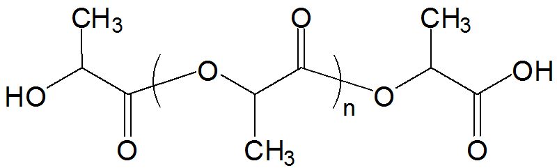
Figure 5: A Diagram showing the Chemical Structure of Polylactic Acid (PLA)

Polylactic Acid is one of the most promising biodegradable polymers owing to its mechanical properties profile, biological properties, such as biocompatibility in contact with living tissues (for example: biomedical applications such as implants, sutures and drug encapsulation) and biodegradable (for example: short – term packaging). According to (Averous, 2008), Polylactic Acid (PLA) can be degraded by abiotic degradation ([Defined Term, 2017] defined Abiotic Degradation as the process in which a substance is converted to simpler products by physical or chemical mechanisms).

(Lopes, Jardini and Filho, 2012) states that “In order for biopolymers to be useful, it is necessary to able to tune the material properties to satisfy engineering constraints”. Polylactic Acid (PLA) exists as a polymeric helix, with an orthorhombic unit cell. ([Encyclopedia Britannica, 2017] describes Orthorhombic system as one of the structural categories system to which crystalline solids can be assigned). Polylactic Acid (PLA) properties depends on the component isomers, processing temperature, annealing time and molecular weight. According to (Lopes, Jardini and Filho, 2012), stereochemistry and thermal history have direct influence on Polylactic (PLA) crystallinity and therefore on its properties in general. Polylactic Acid with poly(L-lactide) PLLA content higher than 90% tends to be crystalline, while the lower optically pure is amorphous.

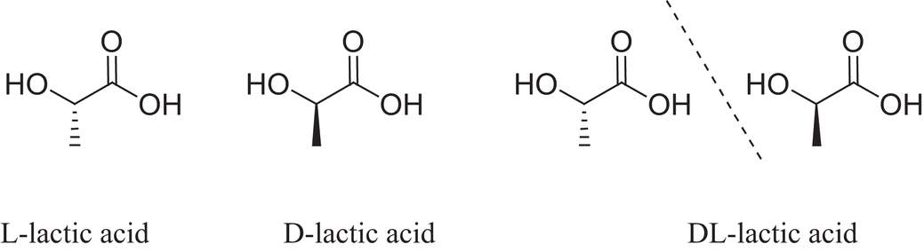
Figure 6: Diagram Showing the Stereoisomers of Polylactic Acid (PLA)

Polylactic Acid is a clear, colourless thermoplastic when quenched from the melt and is similar in many respects to polystyrene. Physical Characteristics such as density, heat capacity, mechanical and rheological properties of PLA are dependent on its transition temperatures. PLA products are soluble in dioxane, acetonitrile, chloroform, methylene chloride, 1,1,2-trichloroethane and dichloroacetic acid. Ethylbenzene, toluene, acetone and tetrahydrofuran only partly dissolve polylactic acid when cold, but they are soluble in these solvents when they are heated to boiling temperatures.

BIODEGRADATION

Biodegradation according to (safeopedia.com, 2017) is defined as a natural process during which fungi, bacteria or other biological organisms break down materials. According (Mohammed, 2017), Biodegradable Polymers are defined as polymers comprised of monomers linked to one another through functional groups and have unstable links in the backbone. They are broken down into biologically acceptable molecules that are metabolized and removed from the body via normal metabolic pathways.

According to (Corning, 1997), Degradation of all polymers follows a sequence in which polymer is first conversion to its monomers, after which monomers are mineralized. Most polymers are too large to pass through cellular membranes, so they must be depolymerized to small monomers before they can be absorbed and biodegraded within microbial cells. The initial breakdown of a polymer can result from a variety of physical, chemical and biological forces with chemical hydrolysis probably being the most important.

Physical forces such as heating or cooling, freezing or thawing, wetting or drying can cause a mechanical damage such as the cracking of polymeric materials. The growth of many fungi can also small-scale swelling and bursting. These physical forces deteriorate the polymer surfaces and create new surfaces for reacting with chemical and biochemical agents. (Corning, 1997) stated that a few synthetic polymers are also depolymerized by microbial enzymes, after which the monomers are absorbed into microbial cells and biodegraded. Depolymerization of most synthetic occurs abiotically, after which biodegradation of the monomers by microorganism proceeds as a secondary process. Abiotic Hydrolysis is the most important reaction for starting the environmental degradation of synthetic polymer which include polylactic (PLA) and copolymers, where hydrolysis acts as the initial step of splitting the polymers into its monomers, after which the monomers can be biodegraded. According (Avérous and Pollet, 2012), the end – products from biodegradation are; CO2 (carbon-dioxide), new biomass and water (in the presence of oxygen, that is aerobic conditions), or methane (in the absence of oxygen that is anaerobic conditions).

LITERATURE REVIEW

CRYSTALLINITY:

According to (Ahmed et al., 2008), Polylactic Acid (PLA) comes in a wide range of different grades, with a range of various levels of different crystallisation, but however, the higher the crystallisation the better the properties. (Lin Xiao et al.) states that the homopolymer of LA is a white powder at room temperature with Tg and Tm values of about 55oc and 175oc, respectively. High molecular weight PLA is a colourless, glossy, rigid thermoplastic materials with properties similar to polystyrene. The two isomers of LA can produce four distinct materials. Poly-D-Lactic Acid (PDLA), is a crystalline material with a regular chain structure. According to (Lin Xiao et al.), Poly-D-Lactic Acid (PDLA) has a crystalline structure with the melting temperature of 180oc. The Poly-D-Lactic Acid (PDLA) has a glass temperature between 50oc to 60oc with a decomposition temperature of 200oc. They experience elongation at break between 20% to 30% and have a breaking strength between 4.0 to 5.0. Poly-L-Lactic (PLLA) is a hemi crystalline material with a regular chain structure. According to (Lin Xiao et al.), Poly-L-Lactic Acid (PLLA) has a hemi crystalline structure with the melting temperature of 180oc. The Poly-L-Lactic Acid (PLLA) has a glass temperature between 55oc to 60oc with a decomposition temperature of 200oc. They experience elongation at break between 20% to 30% and have a breaking strength between 4.0 to 5.0. Poly-D ,L-lactic Acid (PDLLA) is an amorphous and meso – PLA, obtained by the polymerisation of meso – lactic Acid. According to (Lin Xiao et al.), Poly-D ,L-Lactic Acid (PDLLA) has a hemi crystalline structure with a variable melting temperature. The Poly-D ,L-Lactic Acid (PDLLA) has a variable glass temperature with a decomposition temperature of 185 oc to 200oc. They also have a variable elongation and with a variable breaking strength.

(Ahmed et al., 2008), investigated the thermal analysis of a series of polylactides (PLA) based on the number of average molecular mass and the nature of isomer. (Ahmed et al. 957-964) reported that the glass transition temperature for Poly-L-Lactic Acid (PLLA), was said to be found higher than in Poly-D ,L-lactic Acid (PDLLA). It was stated that samples with semi- crystalline samples display a higher glass transition temperature than amorphous samples with similar molecular weights by (Ahmed et al., 2008). (Ahmed et al., 2008) concluded the fact the thermal analysis of a series of a polylactides indicated that the microstructure, number average molecular mass and isomer type have considerable effects on glass transition temperature, melting and crystallisation behaviour.

(Velazquez-Infante et al., 2012) investigated the effect of the unidirectional drawings on the thermal and mechanical properties of Polylactic Acid (PLA) films with different L-isomer content. The report consisted of the thermoforming process of two different L-isomer content Polylactic (PLA) and studying the influence on the induced morphology and the variation in the thermal and tensile properties. The thermoforming process was simulated with uniaxial tensile tests performed at different temperatures and strain rates, reporting the tensile behaviour before, during and after the test. (Velazquez-Infante et al., 2012) also stated that the properties of each Polylactic Acid (PLA) grades are strongly dependent on its optical purity, ranging from completely crystalline to amorphous materials. It was stated by (Velazquez-Infante et al., 2012) that, the film orientation promoted during the melt stage of the extrusion line had no significant effects on the mechanical properties, whereas orientation induced in a second stage above glass transition temperature resulted in an increase in strength related with an increase in crystallinity ratio. It was concluded and stated by (Velazquez-Infante et al., 2012), the mechanically properties such as modulus, tensile strength, strain at yielding and break) increase with respect to the amorphous film. It shows the crystallinity of the Polylactic Acid (PLA) provides better mechanical properties than amorphous.

(Zhai et al., 2009) investigated the study of crystallisation, meting and Foaming Behaviours of Polylactic Acid in compressed CO2. The isothermal crystallisation test indicated that while polylactic Acid (PLA) exhibited very low crystallisation kinetics under atmospheric pressures, CO2 exposure significantly increased Polylactic Acid (PLA)’s crystallisation rate. (Zhai et al., 2009) investigated the crystallisation behaviour using a regular DSC. According to (Pslc.ws, 2017), DSC is defined as the differential scanning calorimetry is a technique used to study what happens to polymers when heated. (Zhai et al., 2009) investigation stated that the glass transition temperature and the melting temperature of the Polylactic Acid (PLA) was too low induce Polylactic (PLA) crystallisation. At a higher temperature, Polylactic Aid (PLA) could crystallise. As the temperature began to increase, it was stated that the crystallisation rate became faster. (Zhai et al., 2009) concluded that a longer time and narrower temperatures’ window might be needed to induce Polylactic Acid (PLA) crystallisation and at a higher temperature, polylactic Acid will be induced under atmospheric pressure.

(Garancher and Fernyhough, 2012) investigated the crystallinity effects in polylactic acid-based foams. It stated the use of carbon dioxide for the production of polylactic acid foams has been increasingly studied recently. In this study, several commercially available grades of polylactic acid ranging from crystalline to amorphous, were processed using carbon dioxide via the biopolymer network limited process. Crystallinity and thermal behaviour of the foamed samples were characterised using differential scanning calorimetry. The mechanical properties and dimensional stability were also investigated. (Garancher and Fernyhough, 2012) came to a conclusion that crystallinity increase as temperature increases and it was also stated that the crystallisation rate becomes faster as the temperature increased.

(Di Lorenzo, Rubino and Cocca, 2014) investigated the isothermal and non-isothermal crystallisation of poly (L-lactic acid)/poly (butylene terephthalate) blends. It was stated that isothermal and non-isothermal crystallisation of kinetics of poly (L-lactic Acid)/poly (butylene terephthalate) blends containing Poly(L-)lactic Acid (PLLA) as major component is detailed in this contribution. It was also stated that Poly (L-Lactic acid) and poly (butylene terephthalate) are not miscible, but the compatibility of the polymer pair is ensured by interactions between the functional groups of the two polyesters. The addition of Poly (L-Lactic acid) PLLA does not affect the temperature range of crystallisation kinetics of poly (butylene terephthalate) and the addition of poly (butylene terephthalate) does not affect the crystallisation kinetics of Poly (L-Lactic acid). (Di Lorenzo, Rubino and Cocca, 2014) results stated that the crystallisation of poly (butylene terephthalate) occurs at elevated temperature. (Di Lorenzo, Rubino and Cocca, 2014) concluded that PBT crystallizes at temperatures much higher than PLLA, and its crystallization kinetics seems not affected by the presence of the biodegradable polyester, with reference to the investigated composition range and thermal histories. On the other hand, PBT remarkably affects the crystallization rate of PLLA, by promoting the onset of crystal growth. Upon cooling from the melt, crystallization of PLLA in PLLA/PBT blends is initiated at higher temperatures compared to plain PLLA and the attained crystal fraction is sizably higher than in plain PLLA. The enhancement of PLLA crystallization rate is confirmed by optical microscopy analysis, which reveals a much higher nucleation density in the blends, as well by the shape of the DSC exotherm associated to PLLA crystallization, which has a sharp onset in the PLLA/PBT blends, due to simultaneous growth of a large number of crystals. In plain PLLA, instead, only a weak and broad exotherm can be obtained upon crystallization from the melt at the same cooling rate, due to the slow and faint release of heat upon formation of a dwindling number of growing crystals. The faster crystallization rate of PLLA upon addition of PBT is rationalized taking into account that upon cooling PBT crystallizes at temperatures much higher than PLLA; in the blends poly (l-lactic acid) crystals grow in the presence of already crystallized PBT chains, which may act as nuclei for the growth of PLLA spherulites. Moreover, as PLLA and PBT are non-miscible, local orientation of the polymer chains at the interface between the PLLA and PBT phases may favour chain alignment to form crystal nuclei, and may also lead to a decrease of the energy barrier for the formation of heterogeneous nuclei in contact with the interface between the dispersed phase and the matrix, which may also contribute to fasten nucleation of PLLA crystals. The reported data indicate that addition of an immiscible semi crystalline polymer with a high crystallization rate and high crystallization temperature is a successful novel strategy to enhance crystallization kinetics of poly (l-lactic acid), as PLLA based blends containing poly (butylene terephthalate) display considerable improvements in both crystallization rate and crystallinity, compared to plain PLLA.

(Day, Nawaby and Liao, 2006) investigated the differential scanning calorimetry study of the crystallisation behaviour of polylactic acid and its nanocomposites and the data obtained clearly indicates the presence of the nanocomposite particles in the composite material influences the crystallisation of the PLA when crystallised both from the solid amorphous state. (Day, Nawaby and Liao, 2006) concluded that “PLA and its nanocomposite with clay have been shown to follow an Avrami behaviour during isothermal crystallization from the melt and from the amorphous solid state. The Avrami exponents ‘n’ in all cases were about two. The values for the crystallization half-times show that the isothermal crystallization rate of PLA is greatly enhanced by the presence of nano clay particles within the matrix, especially when crystallized from the melt as would be the case under conventional processing conditions. For example, when the materials were crystallized from the melt in the temperature range from 120–130°C the crystallization rate for the composite material was approximately 15 to 20 times faster than that for the neat

PLA. Meanwhile in both cases the maximum crystallization rates observed were in the region of 105 –125°C, with that for the neat PLA being closer to 105°C. It was also interesting to note that prolonged heating at 200°C for times up to 60 min affected the crystallization behaviour of the two samples in completely different manners. For example, the crystallization rate for the neat PLA was noted to increase with prolonged exposure at 200°C, while the rate for the composite sample was noted to decrease.”

From all the research found, the motion that states crystallinity in polymers increases as temperature increases was supported.

POLYLACTIC (PLA) DEGRADATION

According to (Arutchelvi et al., 2008), Polymeric materials released into the environment can undergo physical, chemical and biological degradation or combination of all these due to the presence of moisture, air, temperature, light (photo – degradation), high energy radiation (UV, γ – radiation) or microorganism (bacteria or fungi). The rates of chemical and physical degradation are higher when compared to that of biodegradation. Biodegradability of the polymer is essentially determined by the availability of functional group that increases hydrophilicity. It is also size, molecular weight and the density of the polymer also essentially determined the biodegradation. The amount of crystalline and amorphous regions, the structural complexity such as linearity or presence of branching in the polymer. The presence of easily breakable bonds such as ester or amide bonds as against carbon – carbon bonds. Molecular composition and the nature and physical form of the polymer such as whether it is in the form of films, pellets, powder or fibres.

(Mitchell and Hirt, 2014), investigated the degradation of Polylactic Acid (PLA) fibres at elevated temperature and humidity. It was stated that the hydrolytic degradation of polylactic Acid (PLA) devices has previously been reported as size dependent for devices such as plates, microspheres and films. The degradation of fibres was evaluated based on changes in the total weight, crystallinity and molecular weight of the samples. The aim of the report was to investigate the effect of the fibre diameter on the degradation characteristics of PLA fibres exposed to elevated temperature corresponding to less, comparable, and greater than the glass transition temperature. (Mitchell and Hirt, 2014) concluded that there would have been a difference in the degradation rate of fibres based on the difference in their diameters, but those studies were performed under different conditions. It was also stated with respect to the total weight loss, changes in crystallinity, melting temperature, there was no significant difference observed between the two diameters of fibre tested at any of the temperature. This behaviour is due to the hydrolysis of the PLA chains being reaction controlled with the diffusion timescale, O(R2/D), being many orders of magnitude faster than the reaction timescale, O(1/k). (Mitchell and Hirt, 2014) stated that Previous studies have shown that the activation energy for polyester hydrolysis is greatly affected by increasing the degradation temperature from below to above glass transition temperature. Activation energies obtained by Agrawal et al. above glass transition temperature were nearly half of the activation energies obtained for samples degraded below glass transition temperature. The linear fit of ln(k) vs. 1/T obtained in this study suggests that a constant activation energy could be determined for the range of 40 to 80°C.

(Piemonte and Gironi, 2012) investigated the kinetics of hydrolytic degradation of Polylactic Acid. The focus of the research was to analyse the Polylactic Acid hydrolytic decomposition by means of a kinetic model based on two reactions mechanism. To this end, new experimental data have been gathered in order to investigate a wider temperature range (from 140 to 180 °C) and to extend the water/PLA ratio up to 50 % of PLA by weight. The reported results clearly highlight that more than 95 % of PLA is hydrolysed to water-soluble lactic acid within 120 min, when it is hydrolysed within 160–180 °C. Furthermore, the kinetic constant is highly influenced by reaction temperature. The proposed “two reactions” kinetic mechanism complies satisfactorily with the experimental data under analysis. (Piemonte and Gironi, 2012) concluded and stated that “experimental data on the hydrolytic depolymerization of Polylactic Acid (PLA) in water solutions at different temperatures. More than 100 experimental runs have been carried out to build the three kinetic curves at three different temperatures of industrial interest. A new kinetic model that accounts for both autocatalytic reaction mechanism and two reaction phases theory has also been proposed. The findings clearly highlight that more than 95 % of PLA has been hydrolysed to water-soluble LA within 120 min when hydrolysed in the temperature range of 160–180 °C. Furthermore, the kinetic constants are highly influenced by reaction temperature, for both high and low initial Polylactic Acid (PLA) concentrations. The “two reactions” kinetic mechanism proposed in this paper to analyse the experimental data collected seems to be reliable and therefore useful to develop and optimize the depolymerization process of Polylactic Acid (PLA) to get its monomer”.

(La Mantia et al., 2015) investigated the thermomechanical degradation of Polylactic Acid (PLA) based nanobiocomposite. It stated that Nanobiocomposite are a new class of biodegradable materials with nanometric dispersion of inert particles in a biodegradable polymer matrix that show very interesting properties often very different from those of conventional – filled polymers and biodegradability. It also stated that the presence of nanoparticles slightly increases the thermomechanical degradation of the pure matrix and with increasing time and temperature processing. (La Mantia et al., 2015) concluded that “The effects of the processing conditions on the nanobiocomposite made by Bioflex and organ modified clay are extremely important in determining the morphology and the properties of this system. At the processing temperature of 170°C, the molecular structure of the matrix undergoes some slight degradation, as observed by the small decrease of the viscosity. At the processing temperature of 200°C, the degradation of the matrix is enhanced, but this enhancement of the degradation of the matrix is also due to some small decomposition of the organ modifier of the clay because of the Hoffmann elimination. Indeed, the radicals formed through this decomposition enhance the degradation of the matrix. At this temperature, however, this decomposition is at the first stage, and the evolved CO2 remains entrapped in the clay, increasing the level of intercalation and causing also some exfoliation. The final morphology and properties measured on the nanobiocomposite are then the results of two contrasting effects, namely, a more remarkable degradation of the matrix and a better morphology of the organ modified clay.”

(Pirzadeh, Zadhoush and Haghighat, 2007) investigated the hydrolytic and thermal degradation of PET fibres and PET granule in relation to the effect of crystallisation, temperature and humidity. “The main purpose of this research work was to illustrate the extent of hydrolytic degradation of PET caused by warm water and also to separate the influence of moisture, temperature, and orientation in the degradation process. To achieve this purpose, thermal and hydrolytic degradation of PET (Partly Oriented Yarn (POY), Fully Drawn Yarn (FDY) and granule) at temperatures above and below glass transition temperature (Tg) were carried out using a water bath and an electrical oven. Degradation at lower temperatures from Tg were less prominent and was increased noticeably above Tg. Crystallinity plays a significant role in preventing hydrolytic degradation as the extent of degradation was increased from FDY to granule to POY. X-ray diffraction analysis showed that crystallinity was increased from POY to granule to FDY”. (Pirzadeh, Zadhoush and Haghighat, 2007) concluded that the rate of hydrolytic degradation increased with increasing temperature and degradation rates were prominent only at temperature above the glass transition temperature of PET sample.

AIMS AND OBJECTIVE:

From previous studies, it can be seen clearly seen that temperature affects polylactic acid (PLA) in diverse ways such as degradation, crystallinity which intends affects the physical and mechanical properties of the resulting polymer. So far, little work has conducted investigating the change in temperature and rate. The project will investigate the effect of temperature on the expansion of the polylactic acid, the crystallisation of the polylactic acid shrinkage force of the polylactic Acid. A better understanding of the effect of temperature would be useful in optimising the Polylactic Acid is by altering the microstructure of the polymer.

METHODOLOGY.

Tensile Testing is one of the most fundamental test for engineering and provides valuable information about a material and its associated properties. These properties can be used for design and analysis of engineering structures, and for developing new materials that better suit aa specified use.

Many of the properties of polymers are measured and recorded in the same manner as metallic materials. Stress – strain, modulus of elasticity, strength, creep, fracture, hardness has the same meaning for polymers as they do for metals. Polymer responses are more temperature dependent than metals and some polymer have unique viscoelastic (elastic flow) properties.

Stress – Strain test in polymers generally result in one of three types of behaviour; Brittle (low temperature thermosetting), Ductile (Elevated temperature thermoplastics), Highly Elastic (elastomers). Temperature can drastically affect a polymer’s stress – strain characteristics.

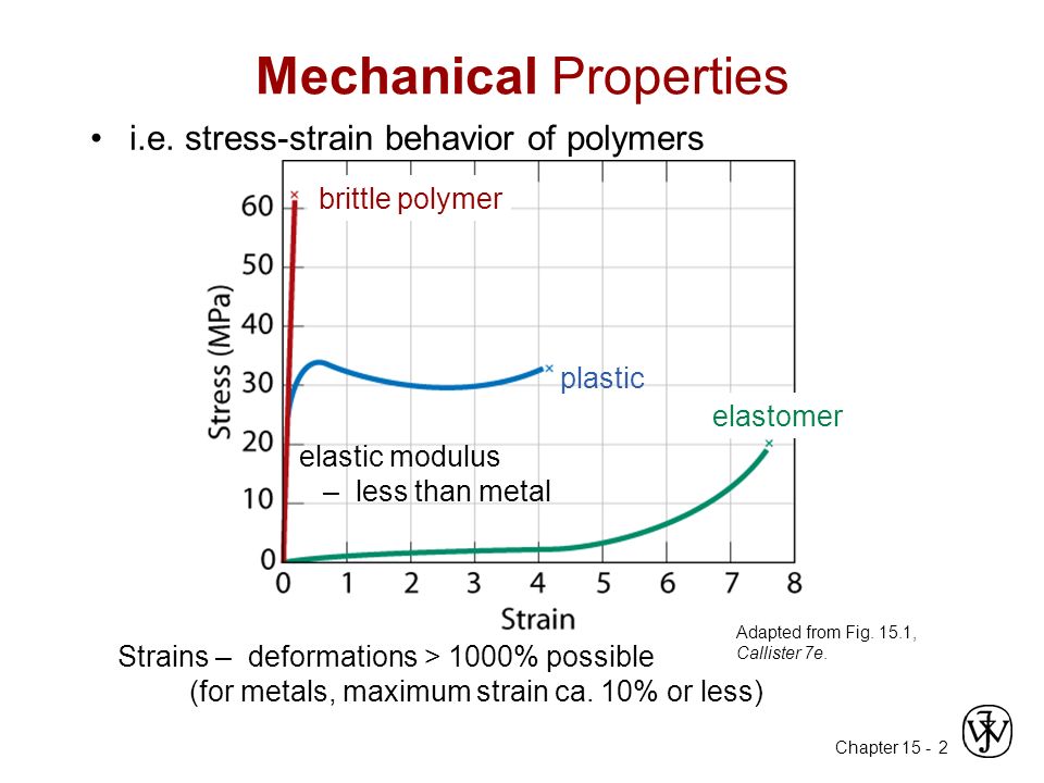
Figure 7: A diagram showing the Graph of Typical Polymer Stress – Strain Behaviour

Creep often occurs in polymers where deformation continues to occur under conditions of constant stress while stress relaxation refers to the decrease in the amount of stress required to main a specific strain. Creep and Stress Relaxation occur because of the relatively gradual sliding of polymer chains with respect to each other when loaded. The modulus of Elasticity varies as a function of temperature for a thermoplastic polymer. There are four distinct regions of viscoelastic behaviour; Rigid, Leathery, Rubbery and Viscous

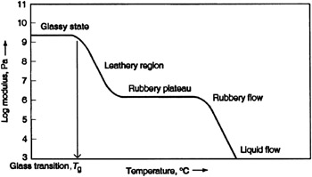
Figure 8:A Diagram Showing the Graph of Polymer Modulus Against Temperature.

Many semi crystalline polymers exhibit a unique deformation process. Deformation proceeds above and below the necked region of a specimen when loaded in tension. This phenomenon is a result of the alignment and straightening of the chains in the necked region, further deformation requires the breaking of bonds.

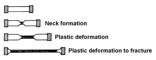
Figure 9: A diagram Showing Deformation of Polymer

The tensile testing laboratory was conducted using an Instron Load frame and the BlueHill data acquisition. The PLA (Polylactic Acid) was tested and heated. The sample was tubular in cross section. Two samples of each materials were tested in the Instron Load frame, and the data gathered into an Excel spreadsheet. The data was used to calculate various properties of each materials, including the elastic modulus, yield strength, ultimate tensile strength. The data was then plotted on engineering stress – strain curves to examine the samples. The purpose of this experiment was to understand the effect of temperature on shape polymer in relation to expansion, crystallisation and shrinkage. This experiment also helped in the familiarization of the Instron Load Frame, BlueHill data acquisition software, and the general steps to performing a tensile test.

MATERIALS USED

POLYLACTIC ACID (PLA)

PLA (Polylactic Acid) according to (Shafer and Lunt, 2011), was discovered in 1932 by Carothers (Du Pont) who produced a low molecular weight product by heating lactic acid under vacuum. The recent advance in fermentation of dextrose, obtained from corn, has led to a dramatic reduction in the cost to manufacture the lactic acid necessary to make Polylactic Acid (PLA) polymers.

(Cargill.com.cn, 2017) stated that NatureWorks LLC is the first company in the world to offer a family of commercially available polymers derived 100 percent annually renewable resources with cost and performance that compete with petroleum based packaging materials and fibres. Its products provide the convenience, look, feel and performance of petroleum based polymers, while minimizing the environmental impact.

According to (Shafer and Lunt, 2011), the primary applications have been identified in fibres and nonwovens, paper coating, films and thermoforming. There are also reports that promises are seem in foams and injection stretch blow moulded containers

EQUIPMENT USED

INSTRON LOAD FRAME

The Instron, also called a screw driven mechanical testing machine, consists of a stationary crosshead, a moving crosshead and a load cell as seen in the diagram figure below. The sample and the in-line load cell are mounted in between these two crossheads. The experiment is performed by measuring the load while a strain is applied to the specimen. Thus, as Instron test is essentially a strain controlled experiment.

The crosshead displacement and the load are translated into stress and strain from the dimensions of the specimen. This machine is fully automatic and computer controlled. The software to operate this machine has been pre-configured for the test.

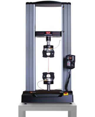
Figure 10: A Diagram showing the equipment Instron Load Frame

The schematic figure of the Instron Load Frame is shown below. The principle of operation is very simple. The sample is deformed by securing it in between a stationary and a moving crosshead. The moving crosshead is generally driven by screw mechanism. The load to achieve deformation in the specimen is measured by the software BlueHill. It can be used for distinct kinds of experiments, example such as, the load and the displacement applied to the specimen can be converted to stress – strain curve; or a bending experiment to measure the load to fracture.

THE VERNIER CALLIPER

Vernier Callipers is an instrument for making very accurate linear measurements and was introduced in 1631 by Pierre Vernier of France. According to (Technologystudent.com, 2017), the Vernier calliper is a precision instrument that can be used to measure internal distances and external distances of a hollow cylinder extremely accurate, the length of a rod or any object, depth of a small beaker.

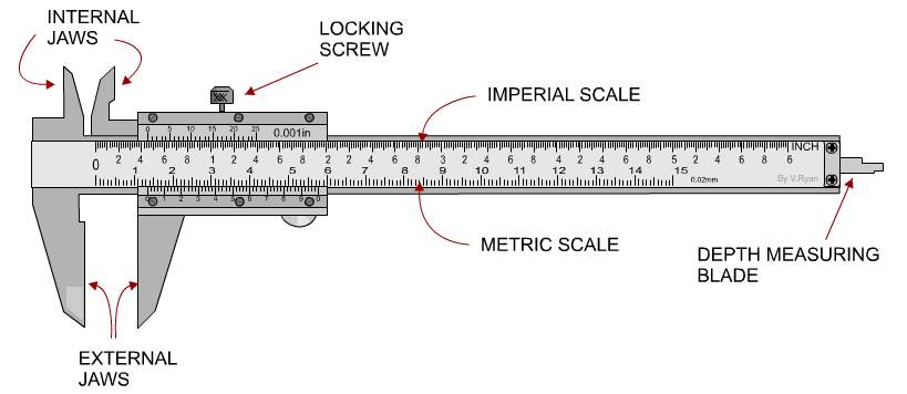
Figure 11: A diagram showing the equipment The Vernier Calliper

STEEL RULE

According to (Using A Steel Rule, 2017), the steel rule is basic measuring tool. A rule is used to measure actual sizes. It is also an instrument used in geometry, technical drawing, printing, engineering and building to measure distances or draw a straight line.

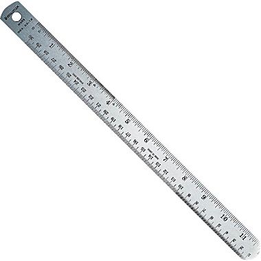
Figure 12: A diagram showing the equipment Steel Rule

DIGITAL THERMOMETER

The digital thermometer allows the measurement of the substrate temperature to be immediately measured. This ensures that the substrate can be maintained at a temperature sufficiently above the dew point to prevent moisture forming on the uncoated surface. It was designed for reliability and ease of use. The digital thermometer has a clear digital display which will give a precise read – out of the temperature.

Figure 13:A Diagram of the equipment Digital Thermometer

FABRIC GLOVES

Fabric and Coated fabric gloves according to (Osha.gov, 2017), are made of cotton or other fabric to provide varying degrees. Fabric Glovesprotect against dirt, slivers, chafing and abrasions. They do not provide sufficient protection for use with rough, sharp or heavy materials. Adding a plastic coating will strengthen some fabric gloves. According to (Osha.gov, 2017), Coated fabric glovesare normally made from cotton flannel with napping on one side. By coating the unnapped side with plastic, fabric gloves are transformed into general-purpose hand protection offering slip-resistant qualities. These gloves are used for tasks ranging from handling bricks and wire to chemical laboratory containers. When selecting gloves to protect against chemical exposure hazards, always check with the manufacturer or review the manufacturer’s product literature to determine the gloves’ effectiveness against specific workplace chemicals and conditions.

Figure 14: A Diagram of the equipment Fabric Gloves

PROCEDURES FOR EXPANSION

Each specimen was measured with the Vernier callipers to determine the diameter of the cross section.
A gage length was determined and scribed.
The BlueHill data acquisition was started and the correct material was chosen.
The load cell was zeroed to ensure that the software measures only the extension and the tensile load applied to the specimen.
The specimen was loaded into the jaw of the Instron load frame so that it was equally spaced between the two clamps.
The Instron Load frame was preloaded using the scroll wheel to ensure that the specimen was properly loaded in the frame and that the specimen did not slip out of the jaws.
The test was started, and the specimen was loaded resulting into measurable strain.
The specimen was heated to an elevated temperature.
At elevated temperature, load was applied and the specimen was stretched.
The data was collected using the BlueHill data acquisition and loaded into a spreadsheet.

The specimen was removed and the crosshead was rest to the initial position to start another tensile test. The testing procedure was repeated for the rest of the specimens.

PROCEDURES FOR CRYSTALLISATION

Each specimen was measured with the Vernier callipers to determine the diameter of the cross section.
A gage length was determined and scribed.
The BlueHill data acquisition was started and the correct material was chosen.
The load cell was zeroed to ensure that the software measures only the extension and the tensile load applied to the specimen.
The specimen was loaded into the jaw of the Instron load frame so that it was equally spaced between the two clamps.
The Instron Load frame was preloaded using the scroll wheel to ensure that the specimen was properly loaded in the frame and that the specimen did not slip out of the jaws.
The test was started, and the specimen was loaded resulting into measurable strain.
The specimen was heated to an elevated temperature and then reduced to lower temperature.
At the low temperature, load was then applied and the specimen was stretched.
The data was collected using the BlueHill data acquisition and loaded into a spreadsheet.
The specimen was removed and the crosshead was rest to the initial position to start another tensile test. The testing procedure was repeated for the rest of the specimens.

The specimen was removed and the crosshead was rest to the initial position to start another tensile test. The testing procedure was repeated for the rest of the specimens

PROCEDURES FOR SHRINKAGE

Each specimen was measured with the Vernier callipers to determine the diameter of the cross section.
A gage length was determined and scribed.
The BlueHill data acquisition was started and the correct material was chosen.
The load cell was zeroed to ensure that the software measures only the extension and the tensile load applied to the specimen.
The specimen was loaded into the jaw of the Instron load frame so that it was equally spaced between the two clamps.
The Instron Load frame was preloaded using the scroll wheel to ensure that the specimen was properly loaded in the frame and that the specimen did not slip out of the jaws.
The test was started, and the specimen was loaded resulting into measurable strain.
The specimen was heated to an elevated temperature.
At the elevated temperature, load was then applied and the specimen was compressed.
The data was collected using a Load cell and loaded into a spreadsheet.

The specimen was removed and the crosshead was rest to the initial position to start another tensile test. The testing procedure was repeated for the rest of the specimens

ELASTICITY ANALYSIS

SPECIMEN 1

The experiment procedures of the load were followed. While loading the specimen into Instron Load Frame, the Bluehill data acquisition software required some parameters. The initial length of the specimen was measured to be 75mm with the outer diameter to be 4.57mm and the wall thickness to be 1.5mm. The initial room temperature was room temperature was 23^oc. The experiment was conducted at a rate of 50mm/min with the temperature heated to 50^oc. The final wall thickness was measured to be 0.79mm and the outer diameter to be 6.08mm.

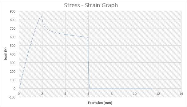
Figure 15: The Stress – strain Graph

ANALYSIS

The figure above shows the stress – strain graph. As the experiment began, there was no load applied thereby resulting to no stress which are both measured to be zero (0) N and zero (0) mm i.e. no yielding. A load was applied which implies that the crosshead began to move and the load was measured to be about 850N while it began to have effect on the strain which implies that the specimen has started expanding to about 2mm. From the graph above, there is a large steep slope indicating fact that necking began. Necking according to (“Necking”), occurs when the cross – sectional area begins to decrease in a localized region of the specimen. The maximum point seen on the graph was recorded and the acknowledged as the maximum stress also known as the Ultimate Stress. The ultimate stress according to (Eduresourcecollection.com, 2017), defines Ultimate stress as the maximum load which can be placed prior to the breaking of the specimen. The load, then decreases to about 700N showing a steep slope in the graph above while the extension increased to about 2.5mm. As extension continued from about 2.5mm to about 6mm, there was a gradual reduction in load from 700N to about 600N as seen in the graph. There was a sudden change in the Load from about 600N to zero (0) N while extension slightly increased from about 6mm to about 6.1mm which implies that the specimen has experienced fracture. The extension increased from about 6.1mm to about 11mm while the load remained the same at zero (0) N implies that the specimen has experienced fracture before the final length was attained

SPECIMEN 2

The experiment procedures of the load were followed. While loading the specimen into Instron Load Frame, the Bluehill data acquisition software required some parameters. The initial length of the specimen was measured to be 75mm with the outer diameter to be 4.57mm and the wall thickness to be 1.5mm. The initial room temperature was room temperature was 23^oc. The experiment was conducted at a rate of 50mm/min with the temperature heated to 55^oc. The final wall thickness was measured to be 0.79mm and the outer diameter to be 6.08mm.

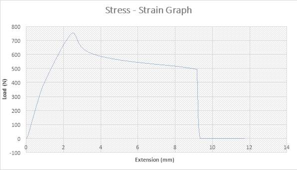
Figure 16: The Stress – strain Graph

ANALYSIS

The figure above shows the stress – strain graph. As the experiment began, there was no load applied thereby resulting to no extension which are both measured to be zero (0) N and zero (0) mm i.e. no yielding. A load was applied which implies that the crosshead began to move and the load was measured to be about 750N while it began to have effect on the strain which implies that the specimen has started expanding to about 2.5mm. From the graph above, there is a large steep slope indicating fact that necking began. The maximum point seen on the graph was recorded and the acknowledged as the maximum stress also known as the Ultimate Stress. The load, then decreases to about 650N showing a small steep slope in the graph above while the extension increased to about 3mm. As extension continued from about 3mm to about 9mm, there was a gradual reduction in load from 650N to about 500N as seen in the graph. There was a sudden change in the Load from about 500N to zero (0) N while extension slightly increased from about 9mm to about 9.1mm which implies that the specimen has experienced fracture. The extension increased from about 9.1mm to about 11.9mm while the load remained the same at zero (0) N implies that the specimen has experienced fracture before the final length was attained

SPECIMEN 3

The experiment procedures of the load were followed. While loading the specimen into Instron Load Frame, the Bluehill data acquisition software required some parameters. The initial length of the specimen was measured to be 75mm with the outer diameter to be 4.57mm and the wall thickness to be 1.5mm. The initial room temperature was room temperature was 23^oc. The experiment was conducted at a rate of 50mm/min with the temperature heated to 55^oc. The final wall thickness was measured to be 0.79mm and the outer diameter to be 6.08mm.

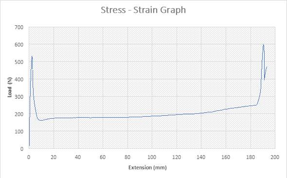
Figure 17:The Stress – strain Graph

ANALYSIS

The figure above shows the stress – strain graph. As the experiment began, there was no load applied thereby resulting to no extension which are both measured to be zero (0) N and zero (0) mm i.e. no yielding. A load was applied which implies that the crosshead began to move and the load was measured to be about 540N while it began to have effect on the strain which implies that the specimen has started expanding to about 3mm. From the graph above, there is a large steep slope indicating fact that necking began. The load, then decreases to about 180N showing a large steep slope in the graph above while the extension increased to about 7mm. As extension continued from about 7mm to about 185mm, there was a gradual increase in load from about 180N to about 250N as seen in the graph. There was a sudden increase in Load from about 250N to about 600N where extension experienced a slight increase from about 185mm to about 190mm. The maximum point seen on the graph was recorded and the acknowledged as the maximum stress also known as the Ultimate Stress. The load, then decreases to about 400N showing a large steep slope in the graph above while the extension increased to about 193mm. There is a slight increase in Load to about 480N where extension also experienced a slight increase to about 195mm. The graph shows that the specimen after the expansion experiment has reached it final length without experiencing fracture.

SPECIMEN 4

The experiment procedures of the load were followed. While loading the specimen into Instron Load Frame, the Bluehill data acquisition software required some parameters. The initial length of the specimen was measured to be 75mm with the outer diameter to be 4.57mm and the wall thickness to be 1.5mm. The initial room temperature was room temperature was 23^oc. The experiment was conducted at a rate of 50mm/min with the temperature heated to 55^oc. The final wall thickness was measured to be 0.79mm and the outer diameter to be 6.08mm.

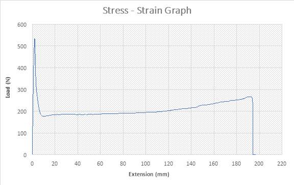
Figure 18:The Stress – strain Graph

ANALYSIS

The figure above shows the stress – strain graph. As the experiment began, there was no load applied thereby resulting to no extension which are both measured to be zero (0) N and zero (0) mm i.e. no yielding. A load was applied which implies that the crosshead began to move and the load was measured to be about 530N while it began to have effect on the strain which implies that the specimen has started expanding to about 3mm. From the graph above, there is a large steep slope indicating fact that necking began. The maximum point seen on the graph was recorded and the acknowledged as the maximum stress also known as the Ultimate Stress. The load, then decreases to about 180N showing a large steep slope in the graph above while the extension increased to about 7mm. As extension continued from about 7mm to about 195mm, there was a gradual increase in load from about 180N to about 270N as seen in the graph. There was a sudden decrease in Load from about 250N to about zero (0) N where extension experienced a slight increase from about 185mm to about 190mm. The sudden change shown in the graph implies that the specimen has experience fracture before it got to its final length.

SPECIMEN 5

The experiment procedures of the load were followed. While loading the specimen into Instron Load Frame, the Bluehill data acquisition software required some parameters. The initial length of the specimen was measured to be 75mm with the outer diameter to be 4.57mm and the wall thickness to be 1.5mm. The initial room temperature was room temperature was 23^oc. The experiment was conducted at a rate of 50mm/min with the temperature heated to 55^oc. The final wall thickness was measured to be 0.79mm and the outer diameter to be 6.08mm.

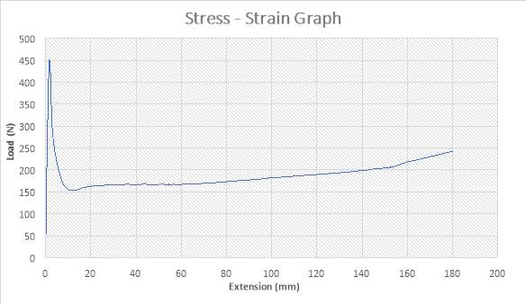
Figure 19: The Stress – strain Graph

ANALYSIS

The figure above shows the stress – strain graph. As the experiment began, there was no load applied thereby resulting to no extension which are both measured to be zero (0) N and zero (0) mm i.e. no yielding. A load was applied which implies that the crosshead began to move and the load was measured to be about 450N while it began to have effect on the strain which implies that the specimen has started expanding to about 2mm. From the graph above, there is a large steep slope indicating fact that necking began. The maximum point seen on the graph was recorded and the acknowledged as the maximum stress also known as the Ultimate Stress. The load, then decreases to about 150N showing a large steep slope in the graph above while the extension increased to about 10mm. As extension continued from about 10mm to about 180mm, there was a gradual increase in load from about 150N to about 240N as seen in the graph. The graph shows that the specimen after the expansion experiment has reached it final length without experiencing fracture.

SPECIMEN 6

The experiment procedures of the load were followed. While loading the specimen into Instron Load Frame, the Bluehill data acquisition software required some parameters. The initial length of the specimen was measured to be 75mm with the outer diameter to be 4.57mm and the wall thickness to be 1.5mm. The initial room temperature was room temperature was 23^oc. The experiment was conducted at a rate of 50mm/min with the temperature heated to 55^oc. The final wall thickness was measured to be 0.79mm and the outer diameter to be 6.08mm.

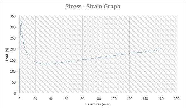
Figure 20:The Stress – strain Graph

ANALYSIS

The figure above shows the stress – strain graph. As the experiment began, there was no load applied thereby resulting to no extension which are both measured to be zero (0) N and zero (0) mm i.e. no yielding. A load was applied which implies that the crosshead began to move and the load was measured to be about 325N while it began to have effect on the extension which implies that the specimen has started expanding to about 2mm. From the graph above, there is a large steep slope indicating fact that necking began. The maximum point seen on the graph was recorded and the acknowledged as the maximum stress also known as the Ultimate Stress. The load, then decreases to about 130N showing a large steep slope in the graph above while the extension increased to about 40mm. As extension continued from about 40mm to about 180mm, there was a gradual increase in load from about 130N to about 200N as seen in the graph. The graph shows that the specimen after the expansion experiment has reached it final length without experiencing fracture.

SPECIMEN 7

The experiment procedures of the load were followed. While loading the specimen into Instron Load Frame, the Bluehill data acquisition software required some parameters. The initial length of the specimen was measured to be 75mm with the outer diameter to be 4.57mm and the wall thickness to be 1.5mm. The initial room temperature was room temperature was 23^oc. The experiment was conducted at a rate of 100mm/min with the temperature heated to 55^oc. The final wall thickness was measured to be 0.79mm and the outer diameter to be 6.08mm.

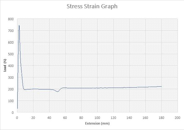
Figure 21: Stress – Strain Graph

ANALYSIS

The figure above shows the stress – strain graph. As the experiment began, there was no load applied thereby resulting to no extension which are both measured to be zero (0) N and zero (0) mm i.e. no yielding. A load was applied which implies that the crosshead began to move and the load was measured to be about 750N while it began to have effect on the strain which implies that the specimen has started expanding to about 4mm. From the graph above, there is a large steep slope indicating fact that necking began. The maximum point seen on the graph was recorded and the acknowledged as the maximum stress also known as the Ultimate Stress. The load, then decreases to about 200N showing a large steep slope in the graph above while the extension increased to about 10mm. As extension continued from about 10mm to about 40mm, there was no effect on the load which remained at 200N as seen in the graph. there was a very slight reduction in load from about 200N to about 180N as the extension increased from 40mm to about 50mm. At extension of 60mm, there was a slight increase in Load from about 180N to about 205N as seen in the graph. The extension increased about 60mm to about 180mm, there was a slight increase in load from 200N to about 210N. The graph shows that the specimen after the expansion experiment has reached it final length without experiencing fracture.

SPECIMEN 8

The experiment procedures of the load were followed. While loading the specimen into Instron Load Frame, the Bluehill data acquisition software required some parameters. The initial length of the specimen was measured to be 75mm with the outer diameter to be 4.57mm and the wall thickness to be 1.5mm. The initial room temperature was room temperature was 23^oc. The experiment was conducted at a rate of 100mm/min with the temperature heated to 55^oc. The final wall thickness was measured to be 0.79mm and the outer diameter to be 6.08mm.

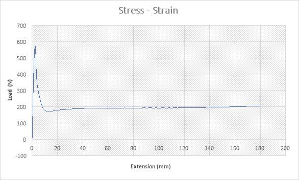
Figure 22: The Stress – Strain Graph

ANALYSIS

The figure above shows the stress – strain graph. As the experiment began, there was no load applied thereby resulting to no extension which are both measured to be zero (0) N and zero (0) mm i.e. no yielding. A load was applied which implies that the crosshead began to move and the load was measured to be about 580N while it began to have effect on the extension which implies that the specimen has started expanding to about 2mm. From the graph above, there is a large steep slope indicating fact that necking began. The maximum point seen on the graph was recorded and the acknowledged as the maximum stress also known as the Ultimate Stress. The load, then decreases to about 180N showing a large steep slope in the graph above while the extension increased to about 10mm. As extension continued from about 10mm to about 180mm, there was a gradual increase in load from about 180N to about 200N as seen in the graph. The graph shows that the specimen after the expansion experiment has reached it final length without experiencing fracture.

SPECIMEN 9

The experiment procedures of the load were followed. While loading the specimen into Instron Load Frame, the Bluehill data acquisition software required some parameters. The initial length of the specimen was measured to be 75mm with the outer diameter to be 4.57mm and the wall thickness to be 1.5mm. The initial room temperature was room temperature was 23^oc. The experiment was conducted at a rate of 50mm/min with the temperature heated to 60^oc. The final wall thickness was measured to be 0.79mm and the outer diameter to be 6.08mm.

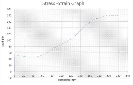
Figure 23: The Stress – Strain Graph

ANALYSIS

SPECIMEN 10

The experiment procedures of the load were followed. While loading the specimen into Instron Load Frame, the Bluehill data acquisition software required some parameters. The initial length of the specimen was measured to be 75mm with the outer diameter to be 4.57mm and the wall thickness to be 1.5mm. The initial room temperature was room temperature was 23^oc. The experiment was conducted at a rate of 50mm/min with the temperature heated to 60^oc. The final wall thickness was measured to be 0.79mm and the outer diameter to be 6.08mm.

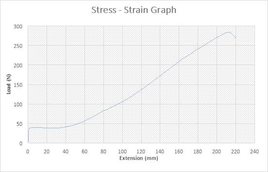
Figure 24:The Stress – Strain Graph

ANALYSIS

The figure above shows the stress – strain graph. As the experiment began, there was no load applied thereby resulting to no extension which are both measured to be zero (0) N and zero (0) mm i.e. no yielding. The load was applied which implies that the crosshead began to move and the load was measured to be about 45N while it began to have effect on the extension which implies that the specimen has started expanding to about 1mm. As extension increases from about 1mm to about 40mm, there was a slight reduction in Load from 45N to about 44N. As extension continued from about 40mm to about 215mm, there was a gradual increase in load from about 44N to about 280N as seen in the graph. The maximum point seen on the graph was recorded and the acknowledged as the maximum stress also known as the Ultimate Stress. There was a very slight reduction in load from about 280 to about 270N as extension experienced a slight increase from about 215mm to about 220mm. The graph shows that the specimen after the expansion experiment has reached it final length without experiencing fracture.

SPECIMEN 11

The experiment procedures of the load were followed. While loading the specimen into Instron Load Frame, the Bluehill data acquisition software required some parameters. The initial length of the specimen was measured to be 75mm with the outer diameter to be 4.57mm and the wall thickness to be 1.5mm. The initial room temperature was room temperature was 23^oc. The experiment was conducted at a rate of 50mm/min with the temperature heated to 60^oc. The final wall thickness was measured to be 0.79mm and the outer diameter to be 6.08mm.

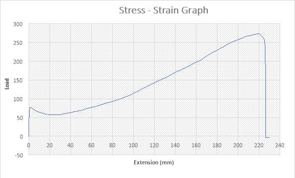
Figure 25:The Stress – Strain Graph

ANALYSIS

The figure above shows the stress – strain graph. As the experiment began, there was no load applied thereby resulting to no extension which are both measured to be zero (0) N and zero (0) mm i.e. no yielding. The load was applied which implies that the crosshead began to move and the load was measured to be about 65N while it began to have effect on the extension which implies that the specimen has started expanding to about 1mm. As extension increases from about 1mm to about 20mm, there was a slight reduction in Load from 65N to about 52N. As extension continued from about 20mm to about 220mm, there was a gradual increase in load from about 52N to about 270N as seen in the graph. The maximum point seen on the graph was recorded and the acknowledged as the maximum stress also known as the Ultimate Stress. There was a sudden change in load from about 270 to about zero (0) N as extension experienced a slight increase from about 220mm to about 225mm. this implies that the specimen has experience fracture.

SPECIMEN 12

The experiment procedures of the load were followed. While loading the specimen into Instron Load Frame, the Bluehill data acquisition software required some parameters. The initial length of the specimen was measured to be 75mm with the outer diameter to be 4.57mm and the wall thickness to be 1.5mm. The initial room temperature was room temperature was 23^oc. The experiment was conducted at a rate of 100mm/min with the temperature heated to 60^oc. The final wall thickness was measured to be 0.79mm and the outer diameter to be 6.08mm.

Figure 26:The Stress – Strain Graph

ANALYSIS

The figure above shows the stress – strain graph. As the experiment began, there was no load applied thereby resulting to no extension which are both measured to be zero (0) N and zero (0) mm i.e. no yielding. The load was applied which implies that the crosshead began to move and the load was measured to be about 90N while it began to have effect on the extension which implies that the specimen has started expanding to about 1mm. As extension increases from about 1mm to about 20mm, there was a slight reduction in Load from 90N to about 55N. As extension continued from about 20mm to about 215mm, there was a gradual increase in load from about 55N to about 240N as seen in the graph. The maximum point seen on the graph was recorded and the acknowledged as the maximum stress also known as the Ultimate Stress. There was a very slight reduction in load from about 240N to about 235N as extension experienced a slight increase from about 215mm to about 220mm. The graph shows that the specimen after the expansion experiment has reached it final length without experiencing fracture.

SPECIMEN 13

The experiment procedures of the load were followed. While loading the specimen into Instron Load Frame, the Bluehill data acquisition software required some parameters. The initial length of the specimen was measured to be 75mm with the outer diameter to be 4.57mm and the wall thickness to be 1.5mm. The initial room temperature was room temperature was 23^oc. The experiment was conducted at a rate of 100mm/min with the temperature heated to 60^oc. The final wall thickness was measured to be 0.79mm and the outer diameter to be 6.08mm.

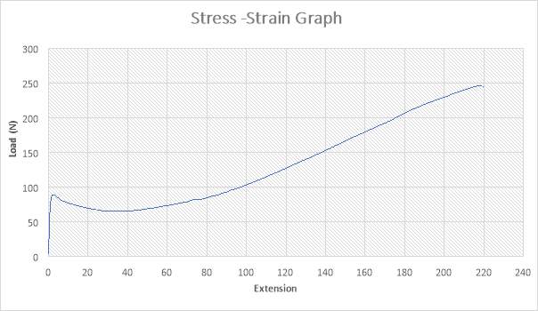
Figure 27: The Stress – strain Graph

ANALYSIS

CRYSTALLISATION ANALYSIS

SPECIMEN 1

The experiment procedures of the load were followed. While loading the specimen into Instron Load Frame, the Bluehill data acquisition software required some parameters. The initial length of the specimen was measured to be 75mm with the outer diameter to be 4.57mm and the wall thickness to be 1.5mm. The initial room temperature was room temperature was 23^oc. The experiment was conducted at a rate of 50mm/min. the temperature was heated to 65^oc and the specimen was left in the hot temperature of 65^oc for about 5 minutes while the oven was still in. After 5 minutes of heating, the temperature was then increased to 100^oc. The final wall thickness was measured to be 0.79mm and the outer diameter to be 6.08mm.

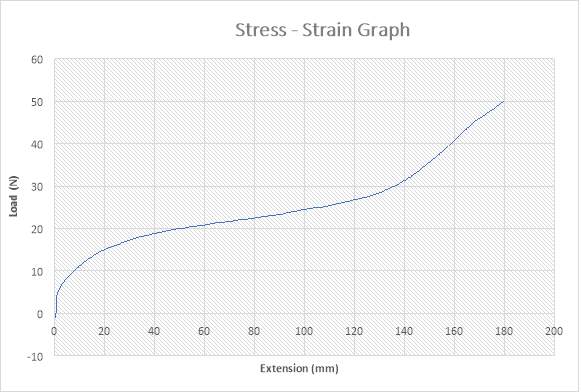
Figure 28: Stress – Strain Graph

ANALYSIS

SPECIMEN 2

The experiment procedures of the load were followed. While loading the specimen into Instron Load Frame, the Bluehill data acquisition software required some parameters. The initial length of the specimen was measured to be 75mm with the outer diameter to be 4.57mm and the wall thickness to be 1.5mm. The initial room temperature was room temperature was 23^oc. The experiment was conducted at a rate of 50mm/min. the temperature was heated to 65^oc and the specimen was left in the hot temperature of 65^oc for about 5 minutes while the oven was still in. After 5 minutes of heating, the temperature was then increased to 100^oc. The final wall thickness was measured to be 0.79mm and the outer diameter to be 6.08mm.

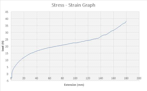
Figure 29: Stress – Strain Graph

ANALYSIS

SPECIMEN 3

The experiment procedures of the load were followed. While loading the specimen into Instron Load Frame, the Bluehill data acquisition software required some parameters. The initial length of the specimen was measured to be 75mm with the outer diameter to be 4.57mm and the wall thickness to be 1.5mm. The initial room temperature was room temperature was 23^oc. The experiment was conducted at a rate of 100mm/min. the temperature was heated to 65^oc and the specimen was left in the hot temperature of 65^oc for about 5 minutes while the oven was still in. After 5 minutes of heating, the temperature was then increased to 100^oc. The final wall thickness was measured to be 0.79mm and the outer diameter to be 6.08mm.

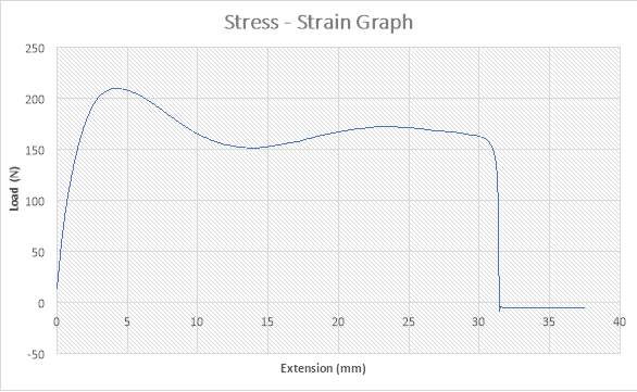
Figure 30: Stress – Strain Graph

ANALYSIS

The figure above shows the stress – strain graph. As the experiment began, there was no load applied thereby resulting to no extension which are both measured to be zero (0) N and zero (0) mm i.e. no yielding. The load was applied which implies that the crosshead began to move and the load was measured to be about 210N while it began to have effect on the extension which implies that the specimen has started expanding to about 4mm. As the expansion increases from about 4mm to about 14mm, there is a slight decrease in load from about 210N to about 150N. As seen in the graph above, there is also an increase in load from about 150N to about 170N as the extension experiences an increase from about 14mm to about 23mm. There is a slight decrease in Load from about 170N to about 160N as the extension experiences increase from about 23mm to about 30mm. At this point of the graph, there is a sudden change in Load from about 160N to about -4N where extension experience increase from about 30mm to about 32mm. This graph above shows that the specimen experienced fracture before reaching its final length. This implies that the crystallisation of this specimen was disrupted.

SPECIMEN 4

The experiment procedures of the load were followed. While loading the specimen into Instron Load Frame, the Bluehill data acquisition software required some parameters. The initial length of the specimen was measured to be 75mm with the outer diameter to be 4.57mm and the wall thickness to be 1.5mm. The initial room temperature was room temperature was 23^oc. The experiment was conducted at a rate of 50mm/min at a temperature of 100^oc. The final wall thickness was measured to be 0.79mm and the outer diameter to be 6.08mm.

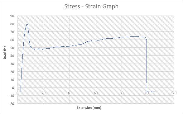
Figure 31: Stress – Strain Graph

ANALYSIS

The figure above shows the stress – strain graph. As the experiment began, there was no load applied thereby resulting to no extension which are both measured to be zero (0) N and zero (0) mm i.e. no yielding. The load was applied which implies that the crosshead began to move and the load was measured to be about 80N while it began to have effect on the extension which implies that the specimen has started expanding to about 7mm. As the expansion increases from about 7mm to about 11mm, there is a slight decrease in load from about 80N to about 49N. As seen in the graph above, there is also an increase in load from about 49N to about 62N as the extension experiences an increase from about 11mm to about 97mm. At this point of the graph, there is a sudden change in Load from about 62N to about -7N where extension experience increase from about 97mm to about 100mm. This graph above shows that the specimen experienced fracture before reaching its final length. This implies that the crystallisation of this specimen was disrupted.

SPECIMEN 5

The experiment procedures of the load were followed. While loading the specimen into Instron Load Frame, the Bluehill data acquisition software required some parameters. The initial length of the specimen was measured to be 75mm with the outer diameter to be 4.57mm and the wall thickness to be 1.5mm. The initial room temperature was room temperature was 23^oc. The experiment was conducted at a rate of 50mm/min at a temperature of 100^oc. The final wall thickness was measured to be 0.79mm and the outer diameter to be 6.08mm.

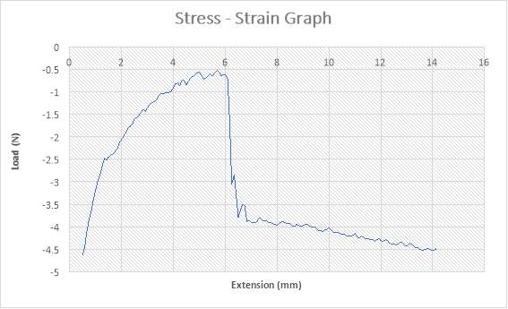
Figure 32: Stress – Strain Graph

ANALYSIS

The figure above shows the stress – strain graph. As the experiment began, there was no load applied thereby resulting to no extension which are both measured to be -4.5 N and zero (0) mm i.e. no yielding. The load was applied which implies that the crosshead began to move and the load was measured to be about -2.5N while it began to have effect on the extension which implies that the specimen has started expanding to about 1mm. As the expansion increases from about 1mm to about 6mm, there is a slight increase in load from about -2.5N to about -0.6N. As seen in the graph above, there is a sudden decrease in load from about -0.6N to about -3.8N as the extension experiences an increase from about 6mm to about 6.4mm. There is a slight increase in Load from about -3.8N to about -3.5N as the extension experiences increase from about 6.4mm to about 6.5mm. There is a slight decrease in Load from about -3.5N to about -3.9N where extension experience increase from about 6.5mm to about 6.6mm. At this point of the graph, there is a gradual reduction in load from about -3.9N to about -4.5N as extension experience increase from about 6.6m to about 14mm. This graph above shows that the specimen experienced fracture before reaching its final length. This implies that the crystallisation of this specimen was disrupted.

SPECIMEN 6

The experiment procedures of the load were followed. While loading the specimen into Instron Load Frame, the Bluehill data acquisition software required some parameters. The initial length of the specimen was measured to be 75mm with the outer diameter to be 4.57mm and the wall thickness to be 1.5mm. The initial room temperature was room temperature was 23^oc. The experiment was conducted at a rate of 50mm/min at a temperature of 100^oc. The final wall thickness was measured to be 0.79mm and the outer diameter to be 6.08mm.

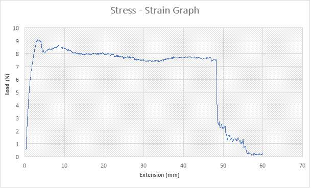
Figure 33: Stress – Strain Graph

ANALYSIS

The figure above shows the stress – strain graph. As the experiment began, there was no load applied thereby resulting to no extension which are both measured to be zero (0) N and zero (0) mm i.e. no yielding. The load was applied which implies that the crosshead began to move and the load was measured to be about 9N while it began to have effect on the extension which implies that the specimen has started expanding to about 4mm. As the expansion increases from about 4mm to about 5mm, the load was a little bit stable. There is a slight decrease in load from about 9N to about 8N as extension increases from 5mm to about 6mm. As seen in the graph above, there is a slight increase in load from about 8N to about 8.5N as the extension experiences an increase from about 6mm to about 10mm. There is a slight decrease in Load from about 8.5N to about 7.5N as the extension experiences increase from about 10mm to about 49mm. At this point of the graph, there is a sudden change in Load from about 7.5N to about 2.8N where extension experience increase from about 49mm to about 49.5mm. At this point of the graph, there is a gradual reduction in load from about 2.8N to about 0.1N as extension experience increase from about 49.5m to about 55mm This graph above shows that the specimen experienced fracture before reaching its final length. This implies that the crystallisation of this specimen was disrupted.

SHRINKAGE FORCE ANALYSIS

SPECIMEN 1

The experiment procedures of the load were followed. While loading the specimen into Instron Load Frame, the Bluehill data acquisition software required some parameters. The initial length of the specimen was measured to be 180mm with the outer diameter to be 4.57mm and the wall thickness to be 1.5mm. The initial room temperature was room temperature was 23^oc. The experiment was conducted at a rate of 50mm/min with the temperature measured to be 55^oc. The final wall thickness was measured to be 0.79mm and the outer diameter to be 6.08mm. The Shrinkage force was measured using a loading cell which was attached to the crosshead of the Instron.

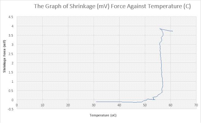
Figure 34:The Graph of Shrinkage(mV) Force against Temperature (C)

ANALYSIS

The figure above shows the graph of the shrinkage force against temperature. As the experiment began, the shrinkage load was measured to about -0.1mV as the specimen just started to experience heating. As the temperature increased from about 31^oc to about 49^oc, there is a very slight decrease in shrinkage force from about -0.1mV to about -0.2mV. As seen in the graph above, there is a slight increase in shrinkage force from about -0.2mV to about 0 showing that the specimen has begun to experience compression or shrinkage while the temperature increased from about 49^oc to about to about 54^oc. At the temperature of 54^oc, the shrinkage force increased from about 0mV to about 0.1mV while temperature remained the same. There was an increase in shrinkage force from about 0.1mV to about 0.5 mV as temperature also experienced an increased from about 54^oc to about 57^oc. While temperature remained at 57^oc, there was a significant increase in shrinkage force from about 0.5mV to about 3.9mV as seen in the graph. There was a slight decrease in shrinkage force from about 3.9mV to about 3.7mV as temperature experienced an increase from about 57^oc to about 61^oc. The graph above shows that the specimen successfully underwent shrinkage without a fracture.

SPECIMEN 2

The experiment procedures of the load were followed. While loading the specimen into Instron Load Frame, the Bluehill data acquisition software required some parameters. The initial length of the specimen was measured to be 180mm with the outer diameter to be 4.57mm and the wall thickness to be 1.5mm. The initial room temperature was room temperature was 23^oc. The experiment was conducted at a rate of 100mm/min with the temperature measured to be 55^oc. The final wall thickness was measured to be 0.79mm and the outer diameter to be 6.08mm. The Shrinkage force was measured using a loading cell which was attached to the crosshead of the instron.

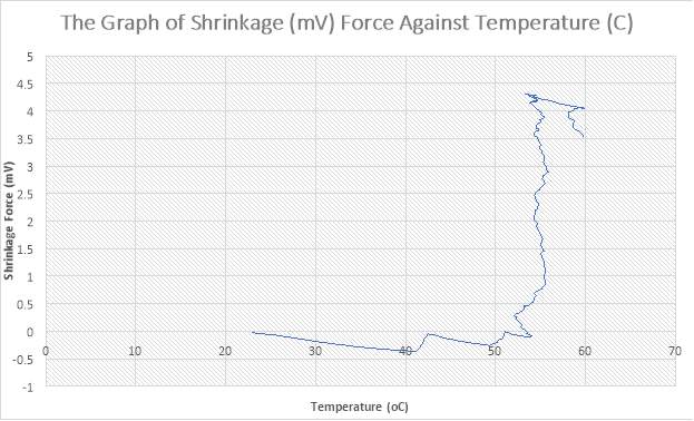
Figure 35: The Graph of Shrinkage(mV) Force against Temperature (C)

ANALYSIS

The figure above shows the graph of the shrinkage force against temperature. As the experiment began, the shrinkage load was measured to about 0mV as the specimen just started to experience heating. As the temperature increased from about 23^oc to about 41^oc, there is a very slight decrease in shrinkage force from about 0mV to about -0.2mV. As seen in the graph above, there is a slight increase in shrinkage force from about -0.2mV to about 0 showing that the specimen has begun to experience compression or shrinkage while the temperature increased from about 42^oc to about to about 43^oc. There is a slight decrease in shrinkage force from about 0mV to about -0.15 mV as temperature experienced an increase from about 43^oc to about to about 50^oc. At the temperature of about 50^oc, there is a slight increase in shrinkage force from about -0.15mV to about 0mV as the temperature also increase from about 50^oc to about 52^oc. There is a slight decrease in shrinkage force from about 0mV to about -0.05 mV as temperature experienced an increase from about 52^oc to about to about 54^oc. At the temperature of 54^oc, the shrinkage force increased from about 0mV to about 0.3mV while temperature experience a slight reduction from 54^oc to about 53^oc. There was an increase in shrinkage force from about 0.3mV to about 0.8 mV as temperature also experienced an increased from about 53^oc to about 55^oc. While temperature remained at 55^oc, there was a significant increase in shrinkage force from about 0.8mV to about 4.3mV as seen in the graph. There was a slight decrease in shrinkage force from about 4.3mV to about 4.0mV as temperature experienced an increase from about 55^oc to about 60^oc. There was a slight decrease in shrinkage from about 4.0mV to about 3.9mV as the temperature also experienced as slight reduction from about 60^oc to about 58^oc. There is an increase in temperature from about 58^oc to about 59.5^oc as the shrinkage force experiences a decrease from about 3.9mV to about 3.6mV as shown in the graph. The graph above shows that the specimen successfully underwent shrinkage without a fracture.

SPECIMEN 3

The experiment procedures of the load were followed. While loading the specimen into Instron Load Frame, the Bluehill data acquisition software required some parameters. The initial length of the specimen was measured to be 220mm with the outer diameter to be 4.57mm and the wall thickness to be 1.5mm. The initial room temperature was room temperature was 23^oc. The experiment was conducted at a rate of 50mm/min with the temperature measured to be 60^oc. The final wall thickness was measured to be 0.79mm and the outer diameter to be 6.08mm. The Shrinkage force was measured using a loading cell which was attached to the crosshead of the instron.

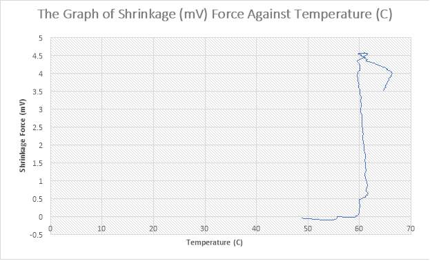
Figure 36: The Graph of Shrinkage(mV) Force against Temperature (C)

ANALYSIS

The figure above shows the graph of the shrinkage force against temperature. As the experiment began, the shrinkage load was measured to about 0mV as the specimen just started to experience heating. As the temperature increased from about 49^oc to about 55^oc, there is a very slight decrease in shrinkage force from about 0mV to about -0.1mV. As seen in the graph above, there is a slight increase in shrinkage force from about -0.1mV to about 0mV showing that the specimen has begun to experience compression or shrinkage while the temperature increased from about 55^oc to about to about 56^oc. As temperature increased from about 56^oc to 60^oc, the shrinkage force remained the same at about 0mV. At the temperature of about 60^oc, there is a slight increase in shrinkage force from about 0mV to about 0.5mV as the temperature remained the same. There is a slight increase in shrinkage force from about 0.5mV to about 0.6 mV as temperature experienced an increase from about 60^oc to about to about 61^oc. While temperature remained at 61^oc, there was a significant increase in shrinkage force from about 0.6mV to about 4.5mV as seen in the graph. There was a slight decrease in shrinkage force from about 4.5mV to about 4.45mV as temperature experienced a decrease from about 61^oc to about 60^oc. There was a slight decrease in shrinkage from about 4.45mV to about 4.0mV as the temperature experienced as slight increase from about 60^oc to about 65^oc. There is a slight reduction in temperature from about 65^oc to about 63^oc as the shrinkage force experiences a decrease from about 4mV to about 3.6mV as shown in the graph. The graph above shows that the specimen successfully underwent shrinkage without a fracture.

SPECIMEN 4

The experiment procedures of the load were followed. While loading the specimen into Instron Load Frame, the Bluehill data acquisition software required some parameters. The initial length of the specimen was measured to be 220mm with the outer diameter to be 4.57mm and the wall thickness to be 1.5mm. The initial room temperature was room temperature was 23^oc. The experiment was conducted at a rate of 100mm/min with the temperature measured to be 60^oc. The final wall thickness was measured to be 0.79mm and the outer diameter to be 6.08mm. The Shrinkage force was measured using a loading cell which was attached to the crosshead of the instron.

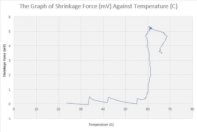
Figure 37: The Graph of Shrinkage(mV) Force against Temperature (C)

ANALYSIS

The figure above shows the graph of the shrinkage force against temperature. As the experiment began, the shrinkage load was measured to about 0mV as the specimen just started to experience heating. As the temperature increased from about 23^oc to about 32^oc, there is a very slight decrease in shrinkage force from about 0mV to about -0.1mV. As seen in the graph above, there is a slight increase in shrinkage force from about -0.1mV to about 0.5mV showing that the specimen has begun to experience compression or shrinkage while the temperature increased from about 32^oc to about to about 34^oc. there is a slight decrease in shrinkage force from about 0.5mV to about 0.1mV while the temperature increased from about 34^oc to about to about 42^oc. There is a slight increase in shrinkage force from about 0.1mV to about 0.5mV as the temperature increased from about 42^oc to about 43^oc. As temperature increased from about 43^oc to 55^oc, the shrinkage force experienced a slight reduction from about 0.5mV to about 0mV. At the temperature of about 55^oc to about 56^oc, there is a slight increase in shrinkage force from about 0mV to about 0.5mV. The shrinkage force remained the same at about 0.5mV as temperature experienced an increase from about 56^oc to about to about 59^oc. While temperature remained at 59^oc, there was a significant increase in shrinkage force from about 0.5mV to about 5.3mV as seen in the graph. There was a slight decrease in shrinkage force from about 5.3mV to about 4.8mV as temperature experienced an increase from about 59^oc to about 68^oc. There was a slight decrease in shrinkage from about 4.8mV to about 3.7mV as the temperature experienced as slight decrease from about 68^oc to about 65^oc. There is a slight increase in temperature from about 65^oc to about 68^oc as the shrinkage force experiences a decrease from about 3.7mV to about 3.6mV as shown in the graph. The graph above shows that the specimen successfully underwent shrinkage without a fracture.

CONCLUSION

The effect of temperature on the Polylactic Acid using expansion, crystallisation and shrinkage force has been studied.

From the analysis, it appears that rate, time and temperature has an influence on the degree of expansion of the material. It was reported that at the temperature of 50^oc and at the rate of 50mm/min, the specimen experienced fracture at a short extension distance. As the temperature was increased to 55^oc and at the rate of 50mm/min, the specimen also experienced a fracture but a longer extension distance. When the final length was reduced to 180mm while the temperature was remained at 55^oc and at the rate of 50mm/min, the final length was reached. There was an increase in the rate and temperature was remained; 100mm/min and 55^oc respectively, the final length was reached but it required a more load or force for expansion. There was an increase in temperature 60^oc and at the rate of 50mm/min, the specimen reached it is final length of 220mm. The rate was increased to 100mm/min and the temperature remained the same at 60^oc; it was reported that the specimen reached its final length of 220mm but it required a lower load or force for expansion. As temperature increased, the force required for expansion reduced there by making it easy for the specimen to reach its final length without experiencing fracture.

From the analysis, it appears that temperature and time has an influence on the degree of crystallinity of the material. It was reported that the specimen was left in the hot temperature of 65^oc for about 5 minutes at the rate 50mm/min. After 5 minutes, the temperature was increased to 100^oc. At this temperature, the specimen experienced crystallisation without fracture at the load of about 50N. At the temperature 100^oc and at the rate of 50mm/min, the specimen experienced fracture before crystallisation was fully occurred. As temperature increased, crystallisation increases there by increasing the mechanical properties of the polymer. When the mechanical properties of a polymer get increased, the polymer tends to experience fracture more.

From the analysis, it appears that temperature and rate has an influence on the degree of shrinkage of the material. It was reported that the experiment was conducted at a rate of 50mm/min with the temperature measured to be 55^oc, the specimen successfully underwent shrinkage without fracture at 3.9mV. It was reported that the experiment was conducted at a rate of 100mm/min with the temperature measured to be 55^oc, the specimen successfully underwent shrinkage without fracture at 3.6mV. It was reported that the experiment was conducted at a rate of 55mm/min with the temperature measured to be 60^oc, the specimen successfully underwent shrinkage without fracture at 3.6mV. It was reported that the experiment was conducted at a rate of 100mm/min with the temperature measured to be 100^oc, the specimen successfully underwent shrinkage without fracture at 3.5mV. As the temperature increase, the shrinkage force decreases.

Studies suggest that temperature has effects on shape memory polymer. A higher temperature leads to an increase in expansion and crystallisation while an increase in temperature leads to a decrease in shrinkage force.

For future research, it would be beneficial to study a wider range of temperature for shorter rates to gain further knowledge on the effect of temperature on shape.

BIBLOGRAPHY

Ahmed, J., Zhang, J., Song, Z. and Varshney, S. (2008). Thermal properties of polylactides. Journal of Thermal Analysis and Calorimetry, 95(3), pp.957-964.

Arutchelvi, J., Sudhakar, M., Arkatkar, A., Doble, M., Bhaduri, S. and Uppara, P. (2008). Biodegradation of polyethylene and polypropylene. 1st ed. [ebook] Mumbai India, pp.10 -20. Available at: http://nopr.niscair.res.in/bitstream/123456789/7326/4/IJBT%207(1)%209-22.pdf [Accessed 22 Apr. 2017].

Averous, L. (2008). Polylactic Acid: Syntesis, Properties and Application. 1st ed. [ebook] pp.434 – 435. Available at: https://biodeg.net/fichiers/Polylactic%20Acid%20Synthesis%20Properties%20and%20Applications.pdf [Accessed 18 Mar. 2017].

Avérous, L. and Pollet, E. (2012). Biodegradable Polymers. Environmental Silicate Nano-Biocomposites, pp.13-39.

Behl, M. and Lendlein, A. (2007). Shape-memory polymers. Materials Today, 10(4), pp.20-28.

Day, M., Nawaby, A. and Liao, X. (2006). A DSC study of the crystallization behaviour of polylactic acid and its nanocomposites. Journal of Thermal Analysis and Calorimetry, 86(3), pp.623-629

Di Lorenzo, M., Rubino, P. and Cocca, M. (2014). Isothermal and non-isothermal crystallization of poly (L-lactic acid)/poly (butylene terephthalate) blends. Journal of Applied Polymer Science, 131(12), pp.1-19.

Garancher, J. and Fernyhough, A. (2012). Crystallinity effects in polylactic acid-based foams. Journal of Cellular Plastics, 48(5), pp.387 – 397.

Hobbs, J. (2004). Crystallization Kinetics. Encyclopedia of Polymer Science and Technology.

Jenkins, A. (1972). Polymer science. 1st ed. Amsterdam [u.a.]: North-Holland, pp.284 – 292.

La Mantia, F., Mistretta, M., Palermo, S., Koci, E. and Ceraulo, M. (2015). Thermomechanical degradation of PLA-based nanobiocomposite. Polymers for Advanced Technologies, 27(3), pp.308-313.

Lin Xiao, Bo Wang, Guang Yang and Mario Gauthier (2012). Poly (Lactic Acid)-Based Biomaterials: Synthesis, Modification and Applications. 1st ed. INTECH Open Access Publisher.

Long, Y., A. shanks, R. and Stachurski, Z. (1995). Kinetics of Polymer Crystallisation. [online] Ac.els-cdn.com.brad.idm.oclc.org. Available at: http://ac.els-cdn.com.brad.idm.oclc.org/007967009500002W/1-s2.0-007967009500002W-main.pdf?_tid=4d74e52e-1c93-11e7-96b8-00000aacb35e&acdnat=1491680644_5597109bf76156dd9e00a675679b3a41 [Accessed 23 Mar. 2017].

Long, Y., Shanks, R. and Stachurski, Z. (1995). Kinetics of polymer crystallisation. Progress in Polymer Science, 20(4), pp.651-701.

Lopes, M., Jardini, A. and Filho, R. (2012). Poly (Lactic Acid) Production for Tissue Engineering Applications. Procedia Engineering, 42, pp.1402-1413.

Majid, M., Revati, R. and Normahira, M. (2017). Biodegeradable Poly (Lactic Acid) Scaffold for Tissue Engineering. 1st ed. [ebook] University Malaysia Perlis (UNIMAP). Available at: https://www.researchgate.net/publication/304114349_Biodegradable_Poly_Lactic_Acid_Scaffold_for_Tissue_Engineering_A_Brief_Review [Accessed 15 Mar. 2017].

Matsuura, K., Nishiyama, T., Sato, E., Yamamoto, M., Kamimura, T., Takahashi, M., Koike, K. and Horibe, H. (2016). Effect of Temperature on Degradation of Polymers for Photoresist Using Ozone Microbubbles. Journal of Photopolymer Science and Technology, 29(4), pp.623-627.

Mitchell, M. and Hirt, D. (2014). Degradation of PLA fibers at elevated temperature and humidity. Polymer Engineering & Science, 55(7), pp.1652-1660.

Owen, K. (2017). Control of Microstructure in Poly-Lactic Acid and The Effect in Biodegradation. 1st ed. Birmingham: University of Birmingham, p.10.

Piemonte, V. and Gironi, F. (2012). Kinetics of Hydrolytic Degradation of PLA. Journal of Polymers and the Environment, 21(2), pp.313-318.

Pirzadeh, E., Zadhoush, A. and Haghighat, M. (2007). Hydrolytic and thermal degradation of PET fibers and PET granule: The effects of crystallization, temperature, and humidity. Journal of Applied Polymer Science, 106(3), pp.1544-1549.

Reiter, G. and Strobl, G. (2007). Progress in understanding of polymer crystallization. 1st ed. Berlin [etc.]: Springer, p.399.

Rosen, S. (1971). Fundamental principles of polymeric materials for practicing engineers. 1st ed. New York: Barnes & Noble, p.41.

Shafer, A. and Lunt, J. (2011). Applications in The Textiles Industry. 1st ed. [ebook] Minnetonka Boulevard, pp.1-8. Available at: http://www.wiley-vch.de/books/biopoly/pdf_v04/bpol4008_235_239.pdf [Accessed 21 Apr. 2017].

Sharples, A. (1966). Introduction to polymer crystallization. 1st ed. London: Edward Arnold LTD, pp.65 – 91.

Using A Steel Rule. (2017). 1st ed. [ebook] littlemachineshop.com, p.1. Available at: http://littlemachineshop.com/instructions/steelrules.pdf [Accessed 4 Apr. 2017].

Velazquez-Infante, J., Gamez-Perez, J., Franco-Urquiza, E., Santana, O., Carrasco, F. and Ll Maspoch, M. (2012). Effect of the unidirectional drawing on the thermal and mechanical properties of PLA films with different L-isomer content. Journal of Applied Polymer Science, 127(4), pp.2661-2669.

Xie, T. (2011). Recent advances in polymer shape memory. Polymer, 52(22), pp.4985-5000.

Zhai, W., Ko, Y., Zhu, W., Wong, A. and Park, C. (2009). A Study of the Crystallization, Melting, and Foaming Behaviors of Polylactic Acid in Compressed CO2. International Journal of Molecular Sciences, 10(12), pp.5381-5397.

REFERNCES

Anon, (2017). Experiment: Polymer. [online] Available at: http://imechanica.org/files/handout7.pdf [Accessed 2 Apr. 2017].

Anon, (2017). Homogenous Nucleation. [online] Available at: http://www.eng.utah.edu/~lzang/images/lecture-10.pdf [Accessed 21 Mar. 2017].

Anon, (2017). Measurement of Length. [online] Available at: http://web.jns.ac.in/worksheet/Measurement%20of%20length.pdf [Accessed 3 Apr. 2017].

Bernard Lynch, B. (2017). Digitalcommons.bucknell.edu. Available at: http://digitalcommons.bucknell.edu/cgi/viewcontent.cgi?article=1244&context=honors_theses [Accessed 19 Apr. 2017].

Cargill.com.cn. (2017). NatureWorks LLC Begins Market Development for Polylatcide (PLA) Polymers in China. [online] Available at: http://www.cargill.com.cn/en/news/NA3000946.jsp [Accessed 21 Apr. 2017].

Chemeddl.org. (2017). Definitions: Chiral. [online] Available at: http://www.chemeddl.org/resources/stereochem/definitions10.htm [Accessed 15 Mar. 2017].

Community.dur.ac.uk. (2017). CRYSTALLISATION KINETICS. [online] Available at: http://community.dur.ac.uk/sharon.cooper/lectures/cryskinetics/handoutsalla.html [Accessed 4 Apr. 2017].

Corning, D. (1997). Degradation of Polymer in Nature. [online] Health Environment & Regulatory Affairs. Available at: http://www.dowcorning.com/content/publishedlit/01-1112-01.pdf [Accessed 24 Mar. 2017].

Crgrp.com. (2017). Shape Memory Polymers | Cornerstone Research Group, Inc... [online] Available at: http://www.crgrp.com/rd-center/shape-memory-polymers [Accessed 23 Apr. 2017].

Defined Term. (2017). DefinedTerm: Abiotic Degradation. [online] Available at: https://definedterm.com/abiotic_degradation [Accessed 5 Apr. 2017].

Deformation of Polymer. (2017). [image] Available at: http://www.che.hw.ac.uk/teaching/B11MS1/Material/Processing/Orient.htm [Accessed 3 Apr. 2017].

Eduresourcecollection.com. (2017). Elastic Limit, Yield Stress, Ultimate Stress, Breaking Stress, Elasticity, Elastic Constants,Modulus of Elasticity,Youngs Modulus,Modulus of Rigidity,Shear Modulus,Bulk Modulus,Working stress,Hookes Law,modulus of elasticity,Youngs Modulus,limit of proportionality,Strength of Materials,question papers,B Tech,BE,semester exams,model questions,enginerring students,projects,seminars,viva voci,Online Educational Resource Collection,university exam model questions,answers,interviews,exams,job. [online] Available at: http://www.eduresourcecollection.com/civil_sm_Elasticity.php [Accessed 5 Apr. 2017].

Encyclopedia Britannica. (2017). amorphous solid | physics. [online] Available at: https://www.britannica.com/science/amorphous-solid [Accessed 10 Mar. 2017].

Encyclopedia Britannica. (2017). orthorhombic system | crystallography. [online] Available at: https://www.britannica.com/science/orthorhombic-system [Accessed 19 Mar. 2017].

Faculty.uscupstate.edu. (2017). Crystallinity. [online] Available at: http://faculty.uscupstate.edu/llever/Polymer%20Resources/Crystalline.htm [Accessed 4 Mar. 2017].

Faculty.uscupstate.edu. (2017). Morphology. [online] Available at: http://faculty.uscupstate.edu/llever/Polymer%20Resources/Morphology.htm [Accessed 4 Mar. 2017].

Faculty.uscupstate.edu. (2017). Polymer. [online] Available at: http://faculty.uscupstate.edu/llever/Polymer%20Resources/MainMenu.htm [Accessed 4 Mar. 2017].

Kohane, D. and Langer, R. (2017). Polymeric Biomaterials in Tissue Engineering.

Merriam-webster.com. (2017). Definition of BIOCOMPATIBILITY. [online] Available at: https://www.merriam-webster.com/dictionary/biocompatibility [Accessed 4 Mar. 2017].

Merriam-webster.com. (2017). Definition of BIOMATERIAL. [online] Available at: https://www.merriam-webster.com/dictionary/biomaterial [Accessed 4 Mar. 2017].

Mohammed (2017). biodegradable polymers. [online] Slideshare.net. Available at: https://www.slideshare.net/Imaad08/biodegradable-polymers-25995228 [Accessed 23 Mar. 2017].

Osha.gov (2017). 1-21. [online] Osha.gov. Available at: http://www.clicksafety.com/ucp/images/pdf/courseware/Chemical%20and%20Liquid%20Resistant%20Gloves.pdf [Accessed 21 Apr. 2017].

PLA Structure. (2015). [image] Available at: http://(PLA Structure) [Accessed 18 Mar. 2017].

Polymer Modulus Versus Temperature. (2017). [image] Available at: http://images.books24x7.com/bookimages/id_15195/fig19_03.jpg [Accessed 2 Apr. 2017].

Pslc.ws. (2017). Differential Scanning Calorimetry. [online] Available at: http://pslc.ws/macrog/dsc.htm [Accessed 20 Apr. 2017].

Ronca, G. (2017). Heterogeneous nucleation in polymer crystallization. [online] Bura.brunel.ac.uk. Available at: http://bura.brunel.ac.uk/handle/2438/7285 [Accessed 22 Mar. 2017].

safeopedia.com. (2017). What is Biodegradation? – Definition from Safeopedia. [online] Available at: https://www.safeopedia.com/definition/622/biodegradation [Accessed 19 Mar. 2017].

Sc01.alicdn.com. (2017). Digital Thermometer. [online] Available at: https://sc01.alicdn.com/kf/HTB1R7QoKVXXXXa8XFXXq6xXFXXXF/industrial-digital-probe-thermometer.jpg [Accessed 4 Apr. 2017].

Sciencing. (2017). Advantages & Disadvantages of Biomaterials. [online] Available at: http://sciencing.com/advantages-disadvantages-biomaterials-8385559.html [Accessed 4 Mar. 2017].

Sites.esm.psu.edu. (2017). necking. [online] Available at: https://sites.esm.psu.edu/courses/emch13d/design/animation/Fnecking.html [Accessed 4 Apr. 2017].

Steel Rule. (2017). [image] Available at: http://www.staples-3p.com/s7/is/image/Staples/s0789173_sc7?$splssku$ [Accessed 4 Apr. 2017].

Study.com. (2017). Stereoisomers: Definition, Types & Examples – Video & Lesson Transcript | Study.com. [online] Available at: http://study.com/academy/lesson/stereoisomers-definition-types-examples.html [Accessed 16 Mar. 2017].

Technologystudent.com. (2017). The Vernier Calliper – Manual Version. [online] Available at: http://www.technologystudent.com/equip1/vernier3.htm [Accessed 3 Apr. 2017].

The Vernier Calliper. (2017). [image] Available at: https://www.google.co.uk/search?q=vernier+caliper+pdf&client=firefox-b&source=lnms&tbm=isch&sa=X&ved=0ahUKEwiKsdev5J3TAhXnIsAKHcNZBgIQ_AUIBigB&biw=596&bih=625#imgrc=NyZIhV8WCK4pGM: [Accessed 3 Apr. 2017].

TheFreeDictionary.com. (2017). polymer. [online] Available at: http://www.thefreedictionary.com/polymer [Accessed 12 Feb. 2017].

Typical Polymer Stress – strain Behaviour. (2017). [image] Available at: http://images.slideplayer.com/31/9715991/slides/slide_2.jpg [Accessed 2 Apr. 2017].

Unterlasslab.com. (2017). Polymer morphology | UNTERLASSLAB. [online] Available at: http://www.unterlasslab.com/research/polymer-morphology.html [Accessed 7 Mar. 2017].

Virginia.edu. (2017). Chapter 15. Polymer Structures. [online] Available at: http://www.virginia.edu/bohr/mse209/chapter15.htm [Accessed 11 Mar. 2017].

Whitwam, R. (2017). New shape-memory polymer can lift 1,000 times its own weight – ExtremeTech. [online] ExtremeTech. Available at: https://www.extremetech.com/extreme/223016-new-shape-memory-polymer-can-lift-1000-times-its-own-weight [Accessed 23 Apr. 2017].

Zhigilei, L. (2017). Nucleation and Kinetic Growth. [online] Available at: http://people.virginia.edu/~lz2n/mse305/notes/Nucleation.pdf [Accessed 22 Mar. 2017].